HAL Id: hal-01882896
https://hal.archives-ouvertes.fr/hal-01882896
Submitted on 27 Sep 2018
HAL is a multi-disciplinary open access
archive for the deposit and dissemination of
sci-entific research documents, whether they are
pub-lished or not. The documents may come from
teaching and research institutions in France or
abroad, or from public or private research centers.
L’archive ouverte pluridisciplinaire HAL, est
destinée au dépôt et à la diffusion de documents
scientifiques de niveau recherche, publiés ou non,
émanant des établissements d’enseignement et de
recherche français ou étrangers, des laboratoires
publics ou privés.
CP-based cloud workload annotation as a preprocessing
for anomaly detection using deep neural networks
Gilles Madi Wamba, Nicolas Beldiceanu
To cite this version:
Gilles Madi Wamba, Nicolas Beldiceanu. CP-based cloud workload annotation as a preprocessing for
anomaly detection using deep neural networks. ITISE 2018 - International Conference onTime Series
and Forecasting, Sep 2018, Granada, Spain. pp.1-12. �hal-01882896�
CP-based cloud workload annotation as a
preprocessing for anomaly detection
using deep neural networks
Gilles Madi Wamba, and Nicolas Beldiceanu
Institut Mines-Telecom Atlantique, LS2N, Nantes, France [email protected]
Abstract. Over the last years, supervised learning has been a subject of great interest. However, in presence of unlabelled data, we face the problem of deep unsupervised learning. To overcome this issue in the context of anomaly detection in a cloud workload, we propose a method that relies on constraint programming (CP). After defining the notion of quasi-periodic extreme pattern in a time series, we propose an algorithm to acquire a CP model that is further used to annotate the cloud workload dataset. We finally propose a neural network model that learns from the annotated data to predict anomalies in a cloud workload. The relevance of the proposed method is shown by running simulations on real-world data traces and by comparing the accuracy of the predictions with those of a state of the art unsupervised learning algorithm.
1
Introduction
With the increase of the use of cloud computing technologies, more and more applications rely on a cloud infrastructure. This model is named Infrastructure as a Service (IaaS). Since failures are common in such large systems [21], the cloud provider needs to ensure the integrity of the infrastructure, prevent failures or fix them as soon as possible.
Most predictive machine learning algorithms rely on historical data to learn a predictive model that can predict the outcome of a given observation. Generally, cloud providers have large quantity of historical data obtained by monitoring some metrics. Such cloud workloads are modelled by time series that are gen-erally not labelled. To address this issue, some data scientists require human intelligence through crowdsourcing services like Amazon Mechanical Turk [20, 17]. The drawback of such approach is its cost in time and money, and even more the reliability of the produced annotations [13]. In the absence of labels, the problem of deep unsupervised learning has been studied in [10]. Most of these approaches rely on k-means clustering [14]. As shown in Section 4.2, a clustering approach is not well suited for anomaly detection in the context of cloud workloads.
In this context, the contribution of this paper is twofold. First we introduce the generic notions of extreme patterns (i.e. pattern occurrences within a time
series for which one or several feature values take very small or very large values relatively to the rest of the time series), and of quasi-periodic pattern group within a time series. Second, we propose a three-step method to solve the problem of predicting malfunction in a cloud data centre infrastructure given its workload: – Using the notion of extreme patterns, we first acquire a constraint program-ming (CP) model that is able to discriminate between a workload presenting a malfunction and one that does not.
– Then we use the acquired CP model to automatically label the historical workload dataset.
– Finally, we train a deep neural network to predict the malfunctions. The rest of the paper is organised as follows. Section 2 provides the necessary background on time series in the context of constraint programming. Section 3 details our main contribution, namely the definition of quasi-periodic extreme patterns and the illustration how to use it to annotate cloud workloads. In Sec-tion 4, we present two methods, the first one based on supervised learning, and the second one based on unsupervised learning (through the k-means algorithm) to predict anomalies in a cloud workload. Finally, we evaluate and compare both models in Section 5 and conclude in Section 6.
2
Background
A time series is a sequence corresponding to measurements taken over time. We use time series to model resource production or consomption, e.g. energy, memory, cpu, bandwidth [6, 15]. These type of time series are constrained by physical or organizational (in general structural) limits as well as by business rules, which restrict the evolution of the series.
Definition 1 (signature). Given a time series x = x1, x2, . . . , xn, the
sig-nature of x is the sequence s = s1, s2, . . . , sn−1, where every si is defined by
(xi < xi+1⇔ si= ‘ < ’) ∧ (xi= xi+1⇔ si= ‘ = ’) ∧ (xi> xi+1 ⇔ si= ‘ < ’).
Definition 2 (s-occurrence, i-occurrence, e-occurrence, found index). Consider a time series x = x1, x2, . . . , xn, its signature sequence s =
s1, s2, . . . , sn−1, a regular expression σ over the alphabet {‘ < ’, ‘ = ’, ‘ > ’}, two
natural numbers b and a, and a subsignature si, si+1, . . . sjwith 1 ≤ i ≤ j ≤ n−2,
forming a maximal word in s matching σ. The s-occurrence of σ is the index sequence i, . . . , j; The i-occurrence of σ is the index sequence i + b, . . . , j; The e-occurrence of σ is the index sequence i + b, . . . , j + 1 − a; The found index is the smallest index k in the interval [i, j] such that the word sisi+1. . . sk is an
occurrence of σ.
An s-occurrence identifies a maximal occurrence of a pattern in a signature sequence, while an i-occurrence identifies a maximal occurrence of a pattern in an input sequence. Note that, by Definition 2, i-occurrences of the same pattern never overlap. The feature value of a pattern occurrence is computed from the e-occurrence, where the constants b and a are used for respectively trimming the left and the right borders of the regular expression σ.
3
Detection of quasi-periodic extreme patterns in CP
Housssam et al. present in [2] a formalisation of arrhythmia detection algorithms. Their algorithm relies on quantitative regular expressions [3] for peak detection. Scholkmann et al. [18] propose another parameter free algorithm for peak detec-tion in periodic or quasi-periodic signals. While those algorithms are designed for peak detection only, our framework [5, 11] is compatible with a large class of regular expressions [11] and offers more than 700 time-series constraints [4].
First, since we aim at extracting relevant maximal occurrence of patterns, we formally define the notion of extreme pattern occurrences. Second, since we also aim at quantifying how regularly such maximal occurrence of patterns appear we define the notion of quasi-periodic extreme pattern. All the corresponding definitions will be illustrated on a concrete example at the end of this section.
3.1 Defining extreme pattern occurrences
In the same way we already synthesise a register automaton for computing the result associated with a time-series function, we also synthesise a register au-tomaton for computing the feature values of each maximal occurrence of a given pattern in a time series in linear time wrt the time-series length. This will be used to extract the extreme feature value, a notion that we now define.
Definition 3 (extreme feature value of a pattern occurrence). Given a regular expression σ, a feature f , a time series ts containing at least one maximal occurrence of σ, and a threshold τ ∈ [0, 1], the ithmaximal occurrence of σ within ts is extreme iff
fσ(i) ∈ [minf,σ(ts), minf,σ(ts) + τ · minf,σ(ts)] ∨
fσ(i) ∈ [maxf,σ(ts) − τ · maxf,σ(ts), maxf,σ(ts)], where
– fσ(i) is the feature value of ith maximal occurrence of σ,
– minf,σ(ts) (resp. maxf,σ(ts)) is the minimum (resp. maximum) feature value
among all maximal occurrences of σ within ts.
Definition 4 (extreme pattern occurrence). Given a regular expression σ and a set of distinct features f1, f2, . . . fk, a maximal occurrence of σ in a time
series ts is an extreme occurrence of σ wrt f1, f2, . . . fk iff all corresponding
feature values are extreme feature values for σ in ts.
3.2 Identifying quasi-periodic extreme patterns
Definition 5 (footprint). Given a time series ts = x0, x1, . . . , xn−1 and a
pattern p, the footprint of p over ts is the sequence fp = q0, q1, . . . , qn−1 of the
same length as ts where each qk∈ fp is an integer between 0 and n such that:
– qk = 0 if index k does not occur in any i-occurrence of the pattern p in the
– qk = j > 0 if index k belongs to the jth i-occurrence of the pattern p when
reading the time series ts.
Definition 6 (footprint distance). The footprint distance between the jth and the (j +1)thmaximal occurrence of a pattern p in a time series ts is the num-ber of zeros in the footprint of p over ts between the end of the jth i-occurrence
of p in ts and the start of the (j + 1)th i-occurrence of p in ts.
Definition 7 (found distance). The found distance between the jth and the (j + 1)th occurrence of a pattern p in a time series ts is the difference between the two corresponding found indices.
Definition 8 (distance). Consider a pattern p for which the length of its small-est occurrence is ` > 0. The distance between the jthand the (j + 1)th maximal occurrence of a pattern p in a time series ts is the footprint distance iff, given any occurrence o of the pattern p, all prefixes and suffixes of o for which the minimum length is greater than or equal to ` are also occurrences of the pattern p, and the found distance otherwise.
Definition 9 (quasi-periodic pattern of order g). Let g and δ be two na-tural numbers with g > 0, p a pattern, ts a time series and opthe sequence of all
maximal occurrences of p in ts. In addition let ep be a subsequence of op of size
at least ` = 3g. Let dp and dp be resp. the minimum and the maximum distance
between any jth and (j + g)th maximal occurrences of p in e
p, with i ∈ [1, ` − g].
Then p is said to be a quasi-periodic pattern of order g and period [dp, dp] iff
1. dp− dp≤ δ,
2. the first maximal occurrence of p ∈ ep is located at a distance d ≤ dp from
the beginning of ts,
3. the last maximal occurrence of p ∈ ep is located at a distance d0 ≤ dp from
the end of ts.
When epcorresponds to all maximal occurrences (resp. all extreme occurrences)
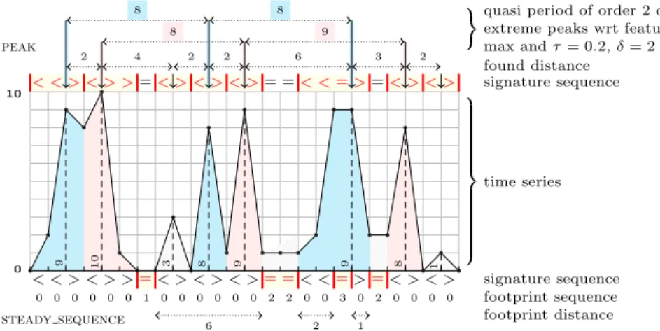
of p then p is a periodic pattern (resp. periodic extreme pattern) of order g. Example 1. We illustrate the previous definitions on the time series 0, 2, 9, 8, 10, 1, 0, 0, 3, 0, 8, 1, 9, 1, 1, 1, 2, 9, 9, 2, 2, 8, 0, 1, 0. For this purpose we consider the peak (resp. steady sequence) pattern defined by ‘ < (= | <)∗(> | =)∗ > ’ (resp. ‘ =+ ’) and by the trimming parameters b = a = 1 (resp. b = a = 0). The eight (resp. four) subsequences outlined in yellow between two vertical red bars on top (resp. at the bottom) of Figure 1 correspond to the eight s-occurrences of the peak (resp. steady sequence) pattern.
The distance of the peak pattern is defined as the found distance since not all large enough suffixes of a maximal occurrence of peak correspond to a peak, i.e. the suffix ‘ >> ’ of the second maximal occurrence of peak ‘ <>> ’ is not a peak itself. Consequently the distances 2, 4, 2, 2, 6, 3, 2 between consecutive max-imal occurrences of peaks are defined as the difference between their correspond-ing found positions, outlined with a vertical arrow in the upper part of Figure 1.
The distance of the steady sequence pattern is defined at the footprint dis-tance since all large enough prefixes and suffixes of ‘ =+’ also correspond to a
steady sequence. Consequently the distances 6, 2, 1 between consecutive maximal occurrences of steady sequences are defined as the difference between the start of a maximal occurrence of the pattern and the end of the maximal occurrence of the previous pattern.
We now focus on the extreme occurrences of the peak pattern wrt the max feature assuming a threshold τ = 0.2. Such feature values 9, 10, 3, 8, 9, 9, 8, 1 are shown in the lower part of Figure 1. Among them only the values 9, 10, 8, 9, 9, 8 belong to the interval [10(1 − τ ), 10], and consequently only the first, second, fourth, fifth, sixth and seventh peak maximal occurrences are extreme. Now as-sume a period threshold δ = 2. Since the minimum/maximum distance between any j and j + 1 positions of extreme pattern occurrences is equal to 2/6, the correspond range 6 − 2 is greater than δ = 2. Consequently the corresponding se-quence of extreme peaks is not quasi-periodic of order 1. But it is quasi-periodic of order 2 because (1) the minimum/maximum distance between any j and j + 2 positions is equal to 8/10, and (2) the first (resp. last) occurrence of peak is not too far from the leftmost (resp. rightmost) border.
0 10 < < > < > >=< > < > < >= =< < = >=< > < > < < > < > >=< > < > < >= =< <=>=< > < > 9 10 3 8 9 9 8 1 0 0 0 0 0 0 1 0 0 0 0 0 0 2 2 0 0 3 0 2 0 0 0 0 2 4 2 2 6 3 2 6 2 1 8 8 8 9
quasi period of order 2 of extreme peaks wrt feature max and τ = 0.2, δ = 2 z }| { z }| { found distance signature sequence time series signature sequence footprint sequence footprint distance peak steady sequence
Fig. 1: Illustrating the notions of signature, found distance, footprint distance, extreme patterns and quasi-periodic extreme patterns wrt the peak=‘ < (= | < )∗(> | =)∗> ’ and steady sequence=‘ =+ ’ patterns
3.3 CP-based time series annotation
In all what follows, a positive (respectively negative) workload trace or time series is a workload trace or time series that do not present any anomaly (respectively that is abnormal). The purpose is to label a set of historical traces as being
either positive or negative. As a first step, we begin with a small set of time series that are prelabelled as positives. From those sample time series, we identify a set Ep = p1, . . . pn of quasi-periodic extreme patterns and we compute their
respective periods. This process is presented in Algorithm 1, where:
– procedure compute extreme occurrences(st, f, p, et) uses Definition 4 to
com-putes the list of all extreme occurrences of the pattern p with respect to the feature f and the threshold et.
– procedure compute period(EV, pt, g) uses Definition 9 to check if the extreme
occurrences in the list EV are quasi-periodic of order g. If yes computes and return the period, else it returns the empty set.
Algorithm 1 Algorithm to acquire a CP model out of positive time series
PROCEDURE LearnCP M odel(S, P, F, et, pt) : (M odel) 1: S: Positive time series set,
2: P : Set of patterns to consider, 3: F : Set of features to consider, 4: et∈ [0, 1]: Extreme value threshold, 5: pt∈ N: Period threshold. 6:
7: st ← {} 8: M odel ← {} 9: for all s ∈ S do
10: st ← stL s . Concatenate all positive time series into st 11: end for
12: g ←max order to consider 13: P eriods ← ∅
14: for all (f, p) ∈ F × P do 15: for all g ∈ [1, g] do
16: EV ← compute extreme occurrences(st, f, p, et) 17: P eriodf,p,g← compute period(EV, pt, g) 18: P eriods ← P eriodsS P eriodf,p,g 19: end for
20: M odel ← M odelS(f, p, P eriods) 21: end for
22: return Model
Each of the remaining traces is labelled as positive if it presents all the quasi-periodic extreme patterns of P , with compatible periods (periods whose inter-section is non-empty) i.e. if it satisfies the CP model acquired by Algorithm 1. The traces that do not satisfy the constraints of the model are labelled as neg-atives. This process is described in Algorithm 2. The next step trains a model that can detect anomalies at run time. The next section details the specificities of our model.
Algorithm 2 Using an acquired CP model to label time series
PROCEDURE LabelT imeSeries(st, M, et, pt) : (ts, label) 1: st: Time series to label,
2: M : Learned model,
3: et∈ [0, 1]: Extreme value threshold, 4: pt∈ N: Period threshold. 5:
6: for all [(f, p, P eriods)] ∈ M × P do
7: EV ← compute extreme occurrences(st, f, p, et) 8: for all P eriodf,p,g∈ P eriods do
9: TSPeriodf ,p,g← compute period(EV, pt, g)
10: if ¬IsCompatible(TSPeriodf ,p,g, P eriodf,p,g) then 11: label ← negative 12: return (st, label) 13: end if 14: end for 15: end for 16: label ← positive 17: return (st, label)
4
Anomalies detection
Given a workload trace, an anomaly is said to occur iff a quasi-periodic extreme pattern, identified by the CP model acquisition step, does not occur at an ex-pected location. In Sections 4.1 and 4.2, we propose two distinct approaches to predict those anomalies. The first one relies on a constrain programming model as a pre-training step while the second one relies on k-means clustering.
4.1 Supervised learning method
Supervised learning [9] is a class of machine learning algorithms that aim at learning a function that computes an output from an input observation. In order to compute that function, supervised learning algorithms rely on input examples together with the expected output value.
In this section we show how we use a deep neural network to detect malfunc-tions in a cloud infrastructure.
Neural network model There is no state-of-the-art method to set the pa-rameters of a neural network [16]. This section presents all the empiric choices relative to our model.
Deep neural network architecture
– Input layer. The choice here is intuitive. Our workload traces are made up of time series representing daily workloads with a time step of 10 minutes. It means that each workload trace is a time series of 144 values, we thus chose 144 as the number of neurons in the input layers.
– Hidden layers. We empirically chose 2 hidden layers of 10 neurons each. – Output layer with two neurons.
Having two neurons in the output layer, the results are interpreted in the following way. The first neuron’s value is the probability that we predict the first category i.e. abnormal, and the second neuron’s value is the probability that we predict the second category normal.
Optimisation
– Activate function. We chose softmax as activation function since we need to output probabilistic values between two discriminative classes [16].
– Stochastic gradient descent. The output y of a neural network given an input X is given by Equation 1 where f is the activate function, W is the weight matrix and B is the bias matrix [16].
y = f (W X + B) (1) To set the parameters W and B during the learning, we used the standard stochastic gradient descent technique with randomly shuffling the training examples. As shown in [7], it performs better than sequential selection of examples that are grouped by classes as it is the case in our model.
4.2 Unsupervised learning method
Unsupervised leaning [12] is a machine learning technique that consists in infer-ring a discriminative function out of an unlabelled set of data.
One of the most popular and yet simple unsupervised learning algorithm is k-means [14]. k-means partitions a set of unlabelled data into k partitions according to a given metric. One difficulty in using k-means is to choose k the number of clusters, as there is no mathematical criterion [19].
In the context of our application, we did not encounter that difficulty, as we already know, that we want to discriminate between two categories, normal and abnormal. Therefore we set k = 2 and we use the Euclidean distance as the distance metric.
The steps required to use the k-means clustering algorithm to predict an anomaly in a time series ts are the following:
1. Learning step: The purpose is to partition the dataset into two clusters. – Select a known normal time series tsn and a known abnormal one tsa.
– Set tsa and tsn to be the initial centroids for k-means clustering.
– Cla and Cln are the two clusters obtained from the dataset, such that
tsa ∈ Cla and tsn∈ CLn
2. Prediction step:
– Computes the centroids ca and cn of Cla and Cln respectively.
– ts is normal (positive) if d(ts, cn) ≤ d(ts, ca) and abnormal otherwise, where d(x, y) is the Euclidean distance between the points x and y.
5
Experiments
In this section, we evaluate each step of our method to predict malfunction in a data centre, we also show the necessity of reinforcing the learned constraint programming model with the neural network of Section 4.1. We further evaluate the unsupervised based learning of Section 4.2.
5.1 Dataset
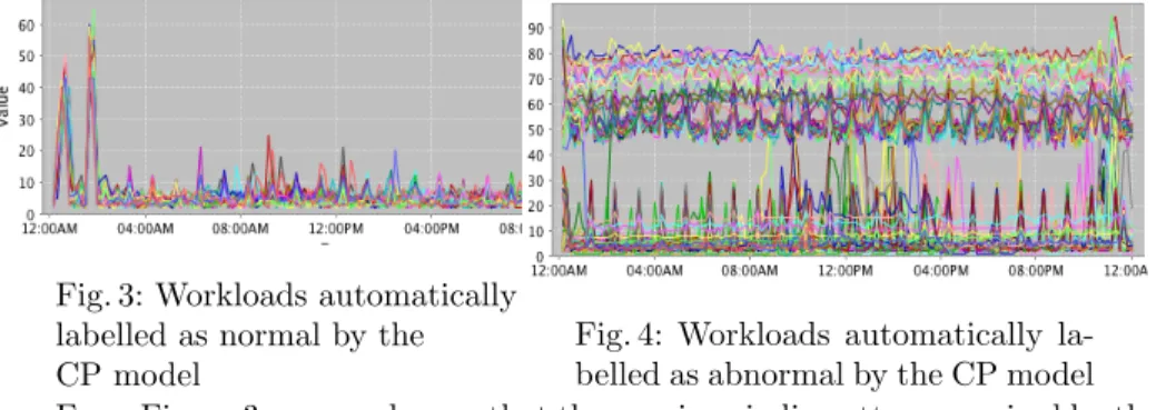
The initial input to our framework is a set of historical workload traces pro-vided by a French SME company specialised in virtualised data centre analysis. Figure 2 shows an instance of raw historical workload traces. Each curve of the figure represents the CPU workload of a VM in a data centre for a whole day in the interval 23rd of February 2017 to 26thof October 2017.
Fig. 2: Unlabeled historical data
5.2 Implementation of the CP based labelling
We implemented Algorithm 2 of Section 3.3 with SICStus Prolog [8].
Figures 3 and 4 shows how the initial unlabelled dataset of Figure 2 is par-titioned into two distinct subsets using Algorithm 2 of Section 3.3.
Fig. 3: Workloads automatically labelled as normal by the CP model
Fig. 4: Workloads automatically la-belled as abnormal by the CP model From Figure 3 we can observe that the quasi-periodic pattern acquired by the CP model is the occurrence of two extreme peaks every day between midnight and 3AM. However, as we will see in Section 5.3, we should take care of some false negative annotations.
5.3 Neural network reinforcement of the CP model
The constraint programming model learned using Algorithm 1 can be used with Algorithm 2 to label workload traces, i.e. it can also be used to detect malfunc-tions in a given workload. However, the quality of the CP model strongly rely on the threshold τ ∈ [0, 1] of Definition 3. This threshold sets the magnitude above and below which a feature value is considered extreme.
Figure 5 shows that the choice of value of τ ∈ [0, 1] is a trade-off between the percentage of false positive and false negative predicted by the model.
Figure 5 induces the following observations:
– For a threshold value above 0.4, i.e. for τ ∈ [0.4, 1] the percentage of false positive predictions of the models grows exponentially. This is not suitable as a false positive prediction is when the model fails to predict a malfunction. – On the other τ ∈ [0, 0.4], the percentage of false negative prediction is close to 100. This is also not suitable as it means that the model predicts a mal-function in almost every workload.
The best trade-off threshold value is thus 0.4. Although τ = 0.4 implies a perfect 0% false positive predictions, it also implies around 12% false negative predictions. This is the reason why we use a neural network on top of the CP model. The CP model provides a good learning base for the neural network.
5.4 Neural network versus K-means prediction
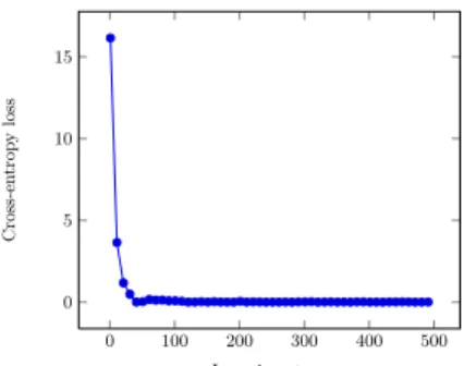
The purpose of the neural network in our framework is to capture hidden struc-tures within the dataset. We implemented the model presented at Section 4.1 in Python using Tensorflow [1]. The amount of false positive and false negative predictions using the so trained neural network are both 0%.
Figure 6 shows how the precision of the model gets high over the learning steps. The precision is evaluated with the cross entropy loss function.We can see that the loss rapidly converges to value 0.
On the other hand, the prediction using the k-means method suffers from the fact that it is based on a notion of closeness through Euclidean distance. The dataset depicted at Figure 2 is therefore separated in two partitions. The direct consequence is the amount of false positive prediction that is above 70%. While a model with a reasonable false negative prediction rate may remain exploitable, the inverse is not desirable. A false negative prediction in our context means that the model fails to predict a malfunction. A 70% false positive rate makes the k-means model not exploitable in this context.
0 0.2 0.4 0.6 0.8 1 0 20 40 60 80 100 Theshold P ercen tage False negative False positive
Fig. 5: False positive against false negative trade-off of the CP model
0 100 200 300 400 500 0 5 10 15 Learning steps Cross-en trop y loss
Fig. 6: Learning graph of the neural network model
6
Conclusion
In this paper we first introduced the generic notions of extreme patterns and quasi-periodic pattern group to capture the behaviour of a time series. Using those notions, we described a machine learning framework for anomaly detec-tion in a cloud workload trace. To overcome the problem of deep unsupervised learning, we proposed a method that relies on constraint programming through the definition of quasi-periodic extreme pattern to annotate the workload time series. After acquiring a constraint programming model, the data set is automat-ically annotated and fed to a neural network for prediction. Experimental results on real workload traces show that state of the art unsupervised learning meth-ods like K-means are not exploitable in our context, and that the combination of a constraint programming model and a neural network produces better results.
Acknowledgement This work was done as part of the PIA HYDDA project funded by the French government. The authors would also like to thank Frederico Alvares from EasyVirt for his active feedback.
References
1. Abadi, M., Barham, P., Chen, J., Chen, Z., Davis, A., Dean, J., Devin, M., Ghemawat, S., Irving, G., Isard, M., et al. (2016). Tensorflow: A system for large-scale machine learning. In OSDI, volume 16. 265–283.
2. Abbas, H., Rodionova, A., Bartocci, E., Smolka, S. A., & Grosu, R. (2017). Quantitative regular expressions for arrhythmia detection algorithms. In Int. Conf. on Computational Methods in Systems Biology. Springer, 23–39. 3. Alur, R., Fisman, D., & Raghothaman, M. (2016). Regular programming
for quantitative properties of data streams. In Thiemann, P., editor, ESOP 2016, volume 9632 of LNCS. Springer, 15–40.
4. Arafailova, E., Beldiceanu, N., Douence, R., Carlsson, M., Flener, P., Rodr´ıguez, M. A. F., Pearson, J., & Simonis, H. (2016). Global constraint catalog, volume ii, time-series constraints. arXiv preprint arXiv:1609.08925. 5. Beldiceanu, N., Carlsson, M., Douence, R., & Simonis, H. (2016). Using
finite transducers for describing and synthesising structural time-series constraints. Constraints, 21(1), 22–40.
6. Beldiceanu, N., Ifrim, G., Lenoir, A., & Simonis, H. (2013). Describing and generating solutions for the EDF unit commitment problem with the modelseeker. In Schulte, C., editor, CP 2013, volume 8124 of LNCS. Springer, 733–748. 7. Bottou, L. (2012). Stochastic gradient descent tricks. In Neural networks: Tricks
of the trade. Springer, 421–436.
8. Carlsson, M., Widen, J., Andersson, J., Andersson, S., Boortz, K., Nils-son, H., & Sj¨oland, T. (1988). SICStus Prolog user’s manual, volume 3. Swedish Institute of Computer Science Kista, Sweden.
9. Caruana, R. & Niculescu-Mizil, A. (2006). An empirical comparison of su-pervised learning algorithms. In Proceedings of the 23rd international conference on Machine learning. ACM, 161–168.
10. Coates, A. & Ng, A. Y. (2012). Learning Feature Representations with K-Means. Springer Berlin Heidelberg, Berlin, Heidelberg. ISBN 978-3-642-35289-8, 561–580. doi:10.1007/978-3-642-35289-8 30.
11. Francisco Rodr´ıguez, M. A., Flener, P., & Pearson, J. (2017). Automatic generation of descriptions of time-series constraints. In Virvou, M., editor, IC-TAI 2017. IEEE Computer Society.
12. Hastie, T., Tibshirani, R., & Friedman, J. (2009). Unsupervised learning. In The elements of statistical learning. Springer, 485–585.
13. Ipeirotis, P. G., Provost, F., & Wang, J. (2010). Quality management on Amazon Mechanical Turk. In Proceedings of the ACM SIGKDD workshop on human computation. ACM, 64–67.
14. Jain, A. K. (2010). Data clustering: 50 years beyond k-means. Pattern recognition letters, 31(8), 651–666.
15. Madi-Wamba, G., Li, Y., Orgerie, A., Beldiceanu, N., & Menaud, J. (2017). Green energy aware scheduling problem in virtualized datacenters. In ICPADS 2017. IEEE Computer Society, 648–655.
16. Nielsen, M. A. (2015). Neural networks and deep learning. Determination Press. 17. Paolacci, G., Chandler, J., & Ipeirotis, P. G. (2010). Running experiments
on amazon mechanical turk.
18. Scholkmann, F., Boss, J., & Wolf, M. (2012). An efficient algorithm for automatic peak detection in noisy periodic and quasi-periodic signals. Algorithms, 5(4), 588–603.
19. Tibshirani, R., Walther, G., & Hastie, T. (2001). Estimating the number of clusters in a data set via the gap statistic. Journal of the Royal Statistical Society: Series B (Statistical Methodology), 63(2), 411–423.
20. Turk, A. M. (2012). Amazon Mechanical Turk. Retrieved August, 17, 2012. 21. Vishwanath, K. V. & Nagappan, N. (2010). Characterizing cloud computing
hardware reliability. In Proceedings of the 1st ACM symposium on Cloud comput-ing. ACM, 193–204.