Science Arts & Métiers (SAM)
is an open access repository that collects the work of Arts et Métiers Institute of Technology researchers and makes it freely available over the web where possible.
This is an author-deposited version published in: https://sam.ensam.eu Handle ID: .http://hdl.handle.net/10985/14215
To cite this version :
Andrea SANSICA, Jean-Christophe ROBINET, Frédéric ALIZARD, Eric GONCALVES - Three-dimensional instability of a ow past a sphere: Mach evolution of the regular and Hopf bifurcations - Journal of Fluid Mechanics - Vol. 855, p.1088-1115 - 2018
Any correspondence concerning this service should be sent to the repository Administrator : archiveouverte@ensam.eu
Three-dimensional instability of a flow past
a sphere: Mach evolution of the regular and
Hopf bifurcations
A. Sansica1,2,†, J.-Ch. Robinet2, F. Alizard3 and E. Goncalves4
1Centre National d’Études Spatiales, Direction des Lanceurs, 52 rue Jacques Hillairet,
Paris 75012, France
2DynFluid Laboratory, Arts et Métiers, 151 Bd. de l’Hopital, Paris 75013, France
3LMFA, Université Lyon 1, CNRS, Ecole Centrale de Lyon, INSA Lyon, 43 Bd. du 11 Novembre 1918,
Villeurbanne 69100, France
4Institut Pprime, ISAE-ENSMA, 1 Av. Clément Ader, Futuroscope Chasseneuil BP 40109 86961, France
(Received 22 December 2017; revised 18 May 2018; accepted 12 August 2018; first published online 24 September 2018)
A fully three-dimensional linear stability analysis is carried out to investigate the unstable bifurcations of a compressible viscous fluid past a sphere. A time-stepper technique is used to compute both equilibrium states and leading eigenmodes. In agreement with previous studies, the numerical results reveal a regular bifurcation under the action of a steady mode and a supercritical Hopf bifurcation that causes the onset of unsteadiness but also illustrate the limitations of previous linear approaches, based on parallel and axisymmetric base flow assumptions, or weakly nonlinear theories. The evolution of the unstable bifurcations is investigated up to low-supersonic speeds. For increasing Mach numbers, the thresholds move towards higher Reynolds numbers. The unsteady fluctuations are weakened and an axisymmetrization of the base flow occurs. For a sufficiently high Reynolds number, the regular bifurcation disappears and the flow directly passes from an unsteady planar-symmetric solution to a stationary axisymmetric stable one when the Mach number is increased. A stability map is drawn by tracking the bifurcation boundaries for different Reynolds and Mach numbers. When supersonic conditions are reached, the flow becomes globally stable and switches to a noise-amplifier system. A continuous Gaussian white noise forcing is applied in front of the shock to examine the convective nature of the flow. A Fourier analysis and a dynamic mode decomposition show a modal response that recalls that of the incompressible unsteady cases. Although transition in the wake does not occur for the chosen Reynolds number and forcing amplitude, this suggests a link between subsonic and supersonic dynamics.
Key words: bifurcation, compressible flows, shock waves
1. Introduction
The onset of large-scale unsteadiness for viscous fluids past axisymmetric bodies represents one of the major subject of study for several modern engineering applications, especially in the field of launcher afterbodies. The complex three-dimensional (3-D) wake dynamics associated with a wide range of axisymmetric bodies (such as disks, spheres or spheroids) shares many similarities and fundamentally differs with respect to its two-dimensional (2-D) counterparts (i.e. in a cylinder wake). In this respect, the wake behind a sphere may be considered as a representative simplified case for axisymmetric bodies. Both numerical simulations and experiments carried out on spheres at low Reynolds numbers reveal the existence of a toroidal recirculation behind the solid body (see Taneda (1956) for the first experimental evidence). Several authors (Magarvey & Bishop 1961; Natarajan & Acrivos 1993; Tomboulides, Orszag & Karniadakis 1993; Wu & Faeth 1993) also show that a first bifurcation occurs when a critical Reynolds number, based on free-stream quantities and the sphere diameter, is reached (Re(1)c ) and yields to the loss of axial symmetry of the steady base flow. The wake is shifted along the normal direction and exhibits a pair of steady streamwise vortices that extend on a very long distance downstream of the body. Although the flow is no longer axisymmetric, a reflectional symmetry of a plane in the streamwise direction still exists. When the Reynolds number is further increased beyond a second critical value (Re(2)c ) the flow undergoes a supercritical Hopf bifurcation and is dominated by a low-frequency shedding of hairpin-like vortices in a Strouhal number range of St ≈ 0.1–0.2 (see Tomboulides et al. (1993), Johnson & Patel (1999), Ormières & Provansal (1999), Schouveiler & Provansal (2002) and Gumowski et al. (2008) for experimental results and direct numerical simulations).
The direct numerical simulations (DNS) of Tomboulides & Orszag (2000), carried out by using a mixed spectral element/Fourier method, show that a primary bifurcation occurs at Re(1)c ≈210 and that the flow remains steady until Re(2)c ≈270. Extensive steady-state axisymmetric numerical simulations and linear stability analyses of flow past a sphere were reported by Ghidersa & Dusek (2000), Tezuka & Suzuki (2006) and Morzy´nski (2009). Within a linear analysis framework, the axisymmetry breaking can be understood by reducing the system into subspaces, each of them being associated with a different azimuthal wavenumber (referenced by m in what follows). As reported by previous authors, the primary bifurcation is seen to arise from a temporally amplified steady mode for the subspace corresponding to m = 1. The bifurcation is then regular. Ghidersa & Dusek (2000) and Meliga, Sipp & Chomaz (2007) also pointed out that the superposition of the steady mode modulated by an arbitrary amplitude onto the base flow induces a loss of symmetry and causes the appearance of a double-threaded wake, observed both experimentally and numerically. The axisymmetric base flow assumption of the linear stability theory can therefore yield inaccurate descriptions of the flow around the second (Hopf) bifurcation, with repercussions for the identification of critical Reynolds number and characteristic frequency.
As underlined by Meliga et al. (2007) and Fabre, Auguste & Magnaudet (2008), the relevance of a stability analysis based on axisymmetric equilibrium states that no longer exist at these Reynolds numbers, is questionable. To fill the gap between the theory and numerical/experimental predictions, Pier (2008) investigates the absolute/convective properties of the planar symmetric basic state under the parallel flow assumption along the streamwise direction. While the existence of an absolutely unstable pocket has been clearly established by the author, the prediction of both
A. Sansica, J.-Ch. Robinet, F. Alizard and E. Goncalves
the critical Reynolds number and the Strouhal number is very rough due to strong non-parallel effects. Trying to overcome the effect of the steady mode on the base flow, Meliga et al. (2007) and Fabre et al. (2008) reinterpreted the Hopf bifurcation as a weakly nonlinear interaction between the stationary mode and the unsteady mode associated with an axisymmetric base flow. While the resulting dynamical system of coupled amplitude equations appropriately depicts the bifurcation diagram, the assumption of simultaneous nearly neutral modes (i.e. for the steady and oscillatory modes) represents an inconsistency since the primary and secondary bifurcations occur at different values of the Reynolds number.
These findings motivate the investigation of the Hopf bifurcation by means of a linear stability analysis that allows a 3-D equilibrium state. Citro et al. (2017) recently carried out a fully 3-D global linear stability analysis without any assumption on the base flow (see Theofilis (2011) for a review) by using a time-stepper approach (see Edwards et al. (1994) and Bagheri, Åkervik & Henningson (2009)). Citro et al. (2017) used an in-house stabilization algorithm called BoostConv (Citro et al.2015) to obtain the planar-symmetric steady base flow that is unstable above the Hopf bifurcation and found a close match between the leading mode and the onset of the unsteadiness.
While the space–time dynamics of large-scale motions for the flow around a sphere is now well predicted by linear stability analysis, little is known about the effect of compressibility on the coherent structures in the wake region. Assuming an axisymmetric base flow configuration independently of the Reynolds number, Meliga, Sipp & Chomaz (2010) examined the effect of compressibility on the linear stability of wake flows, such as an afterbody at zero angle of attack and a sphere. By following the stable and unstable regions in a M–Re plane, they showed that for the supercritical Hopf bifurcation there exists a stabilizing (destabilizing) effect of the Mach number for the afterbody (sphere) flow. As well as not considering the 3-D effects for the base flows around the Hopf bifurcation, their analysis did not account for the presence of shock waves and it was limited up to M ≈ 0.7. A compressible perfect gas with constant specific thermal conductivity and dynamic viscosity related by a unit Prandtl number was considered, limiting some coupling effects between the temperature and momentum equations. Nagata et al. (2016) investigated the evolution of both the mean flow topology and the unsteadiness of the wake behind a sphere at high Mach and low Reynolds numbers conditions by performing nonlinear fully 3-D DNS calculations. The authors showed that an increasing Mach number has a stabilizing effect that causes an axisymmetrization of the flow and/or the disappearance of the unsteady self-sustained periodic behaviour. In a second study at higher Reynolds numbers, Nagata et al. (2018) showed that for a supersonic case at M =1.2 the wake is axisymmetric and steady up to Re = 750 and that the unsteady hairpin shedding only starts at Re = 1000. However, the origins of such phenomena were not discussed in the light of global linear stability theory.
Global stability analysis has been recently shown to be successful for compressible applications of supersonic jets (Ray & Lele 2007; Nichols, Lele & Moin 2009; Beneddine, Mettot & Sipp 2015), parabolic and bluff bodies (Mack, Schmid & Sesterhenn 2008; Meliga et al. 2010), open cavities (Brès & Colonius 2008) and shock-wave/boundary-layer interactions (Crouch, Garbaruk & Magidov 2007; Robinet
2007; Sartor et al. 2015; Guiho, Alizard & Robinet 2016). Although the presence of shock waves was considered in some of these studies, fully 3-D configurations with shock waves are almost non-existent in the literature.
At high Mach and low Reynolds number conditions, as in Nagata et al. (2016,
10−5–10−4 m. Despite the absence of any practical application, a better understanding
of the compressibility effects on the unstable bifurcations of axisymmetric bodies serves to extend the state-of-the-art knowledge but may also provide a first step towards the physical modelling of large scale motion arising in more realistic configurations. In this context, the objective of this work is not only to understand the evolution of the sphere unstable bifurcations with Mach numbers up to supersonic speeds but also to show the capability of global stability analysis in capturing and explaining complex 3-D phenomena in the presence of shock waves and separated regions.
The paper is organized as follows. The numerical methods for DNS and linear global stability are described in §§2 and 3. In §4, the quality of the DNS and time-stepping approach are assessed for the low Mach number regime through detailed comparison with the incompressible case; the regular and Hopf bifurcations are described both in terms of direct numerical simulations and global modes. The supersonic regime is investigated in §5 to analyse the effect of the Mach number on the flow dynamics. Concluding remarks and prospects are given in §6.
2. Problem formulation
2.1. Governing equations
The 3-D Navier–Stokes (N–S) equations for a compressible perfect gas are considered. These equations govern the evolution of the system state q = [ρ, ρu, ρE]T in the
conservative form, where ρ, u and E are the fluid density, the velocity vector and the total energy, respectively. The governing equations can be written in the non-dimensional form as:
∂q
∂t =R(q), (2.1)
where R is the differential nonlinear N–S operator. The explicit form of (2.1) is given in Guiho et al. (2016).
2.2. Stability problem
Linear stability analysis assumes the existence of an equilibrium solution, qb, for the system (2.1) referred to as the base flow and defined by R(qb) = 0. In the following, the base flow qb(x) is assumed to be 3-D, with x = [x, y, z]T representing the array
of the streamwise, vertical and transverse directions, respectively. Using the standard small perturbation technique, the instantaneous flow is decomposed into base flow and small disturbances q(x, t) = qb(x) + εq0(x, t), where ε 1. The resulting equations
are further simplified by considering that the perturbation is infinitesimal, allowing the nonlinear fluctuating terms to be neglected. Thus, the compressible N–S equations become a system of linear partial differential equations defined by
∂q0
∂t =J q
0,
(2.2)
where the vector q0 = [ρ0, ρ0
ub + ρbu0, ρ0Eb + ρbE0]T represents the conservative
perturbation variables and J = ∂R/∂q|qb is the Jacobian operator obtained by
linearizing the N–S operator R around the base flow qb (see Guiho et al. 2016). Assuming a normal mode decomposition, the asymptotic behaviour of a small perturbation is driven by q0(x, t) =
b
the eigenproblem Jbq = λbq. By splitting the eigenvalue into its real and imaginary part λ =σ + iω, the equilibrium state qb is allowed to bifurcate into another solution
if the temporal amplification rate, σ , of the least damped mode becomes positive (in a linear framework).
3. Numerical strategy
3.1. Phoenix code
All numerical simulations in this paper were run with an in-house solver named
PHOENIX (Goncalves & Houdeville 2009), to compute both the linearized and the
full N–S equations. The code solves the compressible N–S equations on multi-block structured grids with a finite-volume approach. Roe’s flux difference splitting scheme (Roe 1981) is employed to obtain advective fluxes at the cell interface for all equations. The monotonic upwind scheme for conservation laws (MUSCL) approach extends the spatial accuracy to third order and, with reference to the supersonic cases, no flux limiters are used. All viscous terms are differentiated by a second-order centred scheme. For unsteady computations, the dual time-stepping method proposed by Jameson (1991) is used. The derivatives with respect to the physical time are discretized using a second-order extrapolation. The boundary conditions used for the steady or unsteady nonlinear calculations (to compute both incompressible and compressible base flow solutions and unsteady cases above the Hopf bifurcation) are: no-slip velocity, adiabatic temperature and pressure extrapolation on the sphere; imposed uniform velocity U∞ at the inflow of the numerical domain; characteristic
boundary conditions at the domain lateral boundaries and outflow to minimize wave reflections.
3.2. Eigenvalue resolution
The same discretization schemes used for the nonlinear N–S equations (2.1) are applied to the set of linearized equations (2.2). However, the spatial schemes as well as boundary conditions need to be adapted to comply to the linearization procedure. As suggested by Crouch et al. (2007), the Roe scheme is based on the Jacobian matrix of the new flux function associated with the linearized equations. Similarly, the same boundary conditions presented in §3.1 for the base flow calculations are linearized and used for the stability analysis. While zero-velocity perturbations are enforced on the sphere wall and domain inlet, the characteristic boundary conditions are evaluated on the base flow solution. To solve this eigenproblem a matrix-free method is used (Edwards et al. 1994; Bagheri et al. 2009). A linear operator P = exp(J1T) that maps q0(tn+1) = Pq0(tn) is introduced, with tn+1 =tn+1T and J the discrete form
of J . In this framework, the action of the operator P can be approximated by a time-marching integration of the linearized N–S equations. The dominant eigenmodes of P are thus extracted by means of an Arnoldi algorithm (Arnoldi 1951; Lehoucq
1997; Barkley, Blackburn & Sherwin 2008) coupled to the linear solver (see Loiseau et al. (2014) and Guiho et al. (2016)). While P and J have the same eigenfunctions, the eigenvalues of J are recovered through λ = log Λ/1T, where Λ denotes an eigenvalue of P. The number of iterations for the Arnoldi technique (Ns) and 1T are
chosen to ensure (i) convergence of the algorithm and (ii) that Nyquist criterion is satisfied. Depending on the case and with the objective to obtain a minimal eigenvalue convergence lower than 10−6, the time step between two consecutive snapshots varies
in the range 1T = (10–130) 1t, with 1t = 0.01 × U∞/Ds, Ds the diameter of the
sphere and U∞ the free-stream velocity, with the dimension of the Krylov subspace
Lz
Ds
Lx
Ly
FIGURE 1. Schematic representation of the computational domain.
Parameters Sphere flow
Free-stream Mach number M =0.1
Free-stream stagnation temperature Ti,∞=287 K Free-stream stagnation pressure Pi,∞=1.013 × 10⁵ Pa
Reynolds number Re ∈ [200; 320]
TABLE 1. Free-stream parameters for the nearly incompressible sphere flow calculations.
4. Regular and Hopf bifurcations of a nearly incompressible flow past a sphere
The numerical investigations first focus on the onset of the unstable bifurcations for a nearly incompressible flow, i.e. at M = 0.1. Several Reynolds numbers around the regular and Hopf bifurcations are considered to describe the breaking of the axisymmetry and onset of unsteadiness, respectively. As well as validating the code against experimental and numerical work present in the literature, especially against Citro et al. (2017) for the Hopf bifurcation since a fully 3-D analysis is performed without any assumptions for the base flow, this section aims at providing a complete picture of the bifurcations in the incompressible regime and introducing the extension to the compressible one presented in the following section.
4.1. Simulation details
The numerical set-up is displayed in figure 1 where the domain configuration and main characteristic scales are presented. The computational domain is composed of 7 blocks and the grid resolution is selected to be (nx, ny, nz) = (112, 112, 112) for each
block. The size of the numerical domain is selected to be (Lx, Ly, Lz) = (20, 10, 10).
A sensitivity study on grid resolution and domain size is presented in appendix A. To avoid any downstream spurious reflection, the grid of the last block is stretched in the streamwise direction downstream of the body. The selected Reynolds numbers are Re = 200, 210, 220 for the characterization of the regular bifurcation and Re = 250, 260, 270, 280, 290, 300, 320 for the Hopf one. The flow conditions are given in table 1. The time and length scales are made dimensionless using U∞/Ds and Ds,
respectively. The dimensionless frequency is defined as St =ω/2π. 4.2. Base flow
The N–S equations are discretized by an implicit scheme and solved by a pseudo-unsteady approach (Jameson 1991). For all the computed base flows the Courant–
1.5
(a) (b)
1.0
0.5 Present
Johnson & Patel (1999) Magnaudet et al. (1995) Tomboulides et al. (1993) Taneda (1956) 0 1.5 1.4 1.3 50 100 Re 150 200 200 240 Re 280 320 Lsep
FIGURE 2. (a) The separation length Lsep is plotted as a function of the Reynolds
number up to Re = 200 and compared against both numerical simulations and experiments. (b) Separation lengths around the two unstable bifurcations for steady axisymmetric (full circles), steady planar-symmetric (empty circles) and time-averaged planar-symmetric (empty diamonds) solutions.
Friedrichs–Lewy (CFL) number is equal to 10 and the steady solutions are converged until the residuals of the state variables in the L2-norm are lower than 10−8.
Before investigating the base flow characteristics around the two bifurcations, the evolution of the separation bubble length is compared against the results reported in Taneda (1956), Tomboulides et al. (1993), Magnaudet, Rivero & Fabre (1995), Johnson & Patel (1999) and Bouchet, Mebarek & Duˆsek (2006) for Reynolds numbers up to Re = 200 (figure 2a). Good agreement is shown between the present and aforementioned results and only (globally stable) steady axisymmetric solutions exist.
Similarly to Bouchet et al. (2006), the calculated separation lengths associated with the Reynolds numbers around the two bifurcations are plotted in figure 2(b).
Above Re = 210, an implicit method is used (Lomax & Steger 1975) where steady axisymmetric flows (full circles fitted by a solid line) are obtained by starting from a very well converged axisymmetric solution (with the residuals of the state variables in the L2-norm below 10−8) and progressively increasing the Reynolds number. Thus,
the solution quickly converges to an axisymmetric one with a longer separation region. However, this strategy does not allow us to calculate well converged solutions far from the threshold of the regular bifurcation and axisymmetric flows could only be obtained up to Re = 260 with this method. These solutions constitute unstable fix points that, through a regular bifurcation, cause the steady wake behind the sphere to become planar-symmetric and are selected to study the evolution of the regular bifurcation with the Reynolds number in §4.3.
Different methods, such as the Newton–Krylov (Edwards et al. 1994) or selective frequency damping method (Åkervik et al. 2006), can be used to obtain the equilibrium solution of the system in (2.1) when unsteady solutions exist above the secondary Hopf bifurcation. However, the implicit scheme combined to a pseudo-unsteady approach at high CFL number used in the present study allows us to filter the unsteadiness and obtain converged steady fixed points. Above the regular bifurcation, the steady wake behind the sphere becomes planar-symmetric and the corresponding length, averaged in the azimuthal direction, is represented by empty circles and fitted by a dashed line. These flows represent nonlinearly saturated
1 0 y z 0 1 2 0 1 2 0 1 x 2 0 1 x 2 -1 1 0 -1 1 0 -1 1 0 -1 (a) (b) (c) (d)
FIGURE 3. Three-dimensional streamlines projected onto (a,b) x–y and (c,d) x–z planes
for the (a,c) Re = 210 and (b,d) Re = 280 cases. The separated region is indicated by the solid black line.
solutions with respect to the regular bifurcation and for Re> 270 constitute unstable fix points that become unsteady through a supercritical Hopf bifurcation. Differently from previous studies that relied on the assumption of axisymmetric base flow for the linear stability analysis, these 3-D planar-symmetric base flows are selected to study the evolution of the secondary Hopf bifurcation in §4.4, as done by Citro et al. (2017). The breaking of the axisymmetry of the base flow solution can be better appreciated in figure 3, where the projections of the 3-D streamlines in the x–y (figure 3a,b) and x–z (figure3c,d) planes are shown for the Re = 210 (figure3a,c) and Re =280 (figure 3b,d) cases. The solid black lines indicate the separation region by plotting the contours of the zero-streamwise velocity. While the flow is axisymmetric at Re = 210, planar symmetry can be observed for the Re = 280 case. Around the secondary Hopf bifurcation, the flow remains symmetric in the x–y plane but the streamlines in the x–z plane spiral asymmetrically downstream of the body and the corresponding wake results slightly bent. These observations are in full agreement with the DNS results provided by Johnson & Patel (1999) for subcritical Reynolds numbers.
Unsteady nonlinear calculations are performed for Re = 280, 300 and 320. Above the supercritical Hopf bifurcation, the flow becomes unsteady and self-sustained hairpin vortices are shed behind the sphere. This solution is time averaged (32 samples in one period at saturation) and a mean flow field is obtained. Although not a fixed point of the system under consideration and mathematically not sound, this solution is used as a base flow in §4.5 to address the issue concerning the correctness of the global stability performed on a fixed point solution in predicting the shedding frequency (Barkley 2006). The size of the recirculation region of the
0.4 0 -0.004 -0.008 -0.004 -0.002 0 0.002 0.004 0.2 0 -0.2 200 210 Re St ß 220 (a) (b)
FIGURE 4. Regular bifurcation: (a) temporal amplification rate versus the Reynolds
number for the least temporally damped/most temporally amplified non-oscillatory global mode; (b) flow case at Re = 210; eigenspectrum in the St–σ plane.
mean flow solution is calculated by further averaging in the azimuthal direction and is represented in figure 2(b) with empty diamonds fitted by a dash-dotted line.
4.3. Regular bifurcation
To study the regular bifurcation, several stability analyses are carried out at Re = 200, 210 and 220. The resulting temporal amplification rate distribution as a function of the Reynolds number in figure 4(a) shows that the axisymmetric base flow is unstable for Reynolds number Re = 210. Small differences of within 5 % are found with respect to the work of Tomboulides & Orszag (2000), Fabre et al. (2008) and Meliga, Sipp & Chomaz (2009) who found the critical value to vary between 210 and 212 (see appendix A). The eigenvalue spectrum for the case at Re =210 is shown in figure 4(b), where the positive growth rate at St = 0 indicates that the corresponding base flow has become unstable and a non-oscillatory mode is temporally amplified.
To better appreciate the azimuthal character of the eigenfunctions and to directly compare with Natarajan & Acrivos (1993), Tomboulides & Orszag (2000) and Tezuka & Suzuki (2006), a transformation of coordinates – from Cartesian (x, y, z) to cylindrical (x, r, θ) – has been applied to transform the streamwise, vertical and transversal (u0, v0, w0) perturbation velocities into streamwise, radial and azimuthal
(v0 x, v
0 r, v
0
θ) ones. Figure 5 shows the iso-surfaces (figure 5a–c) and the projected
contours onto 2-D x–z planes (figure 5d–f ) of the components of the perturbation velocity field (normalized by the maximum of the streamwise velocity component) in the streamwise, radial and azimuthal coordinates associated with this mode. Although in our analysis the hypothesis of axisymmetric base flow is not assumed, the figure shows good agreement with the least stable (m = 1) mode shape reported by Natarajan & Acrivos (1993), Tomboulides & Orszag (2000), Tezuka & Suzuki (2006) and many other authors who adopted a Fourier mode decomposition as q =PM−1
m=0 qm(x, r, t)e imθ,
with x, r and θ the streamwise, radial and azimuthal components. The stationary mode is seen to be dominated by the streamwise velocity disturbances that are located downstream of the sphere and extend up to ≈20Ds. Since the selection of
the plane where the symmetry breaks is equiprobable, the anti-symmetry plane of the eigenmode structures has been rotated to match the x–y plane.
y y y x 0 0 3 -3 3 -3 3 -3 z 5 10 x 0 5 10 x 0 5 10 x 0 5 5 0 5 x x z z z (d) (e) (f)
FIGURE 5. Flow case at Re = 210 for the unstable axisymmetric base flow.
Three-dimensional view of the mode at (σ, St) = (0.683 × 10⁻⁴, 0.0). The iso-surfaces of the (a)
streamwise, (b) radial and (c) azimuthal perturbation velocities are plotted for the levels v0
x= ±0.01, v 0
r= ±0.01 and v 0
θ= ±0.005, respectively. The contours of the (d) streamwise,
(e) radial and ( f ) azimuthal perturbation velocities are plotted on the x–z plane for the levels v0
x= ±0.01, v 0
r= ±0.01 and v 0
θ= ±0.005, respectively. Light and dark grey colours
for positive and negative perturbation velocities, respectively. The sphere is represented in black.
4.4. Supercritical Hopf bifurcation
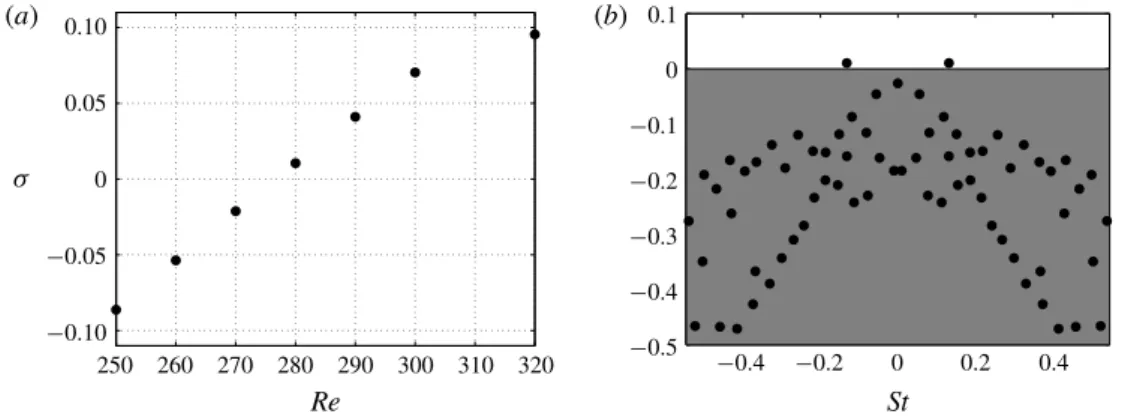
The characterization of the supercritical Hopf bifurcation is done by carrying out several linear stability analyses around Re = 280. It is important to recall that the base flows selected for this analysis are 3-D planar-symmetric solutions and represent unstable fixed points above the secondary Hopf bifurcation. Figure 6(a) reports the evolution of the temporal amplification rate as a function of the Reynolds number and shows that the transition to a time-dependent flow occurs between Re = 270 and 280, consistently with what found experimentally by Ormières & Provansal (1999) and Schouveiler & Provansal (2002) (Re(2)c ≈280) and via DNS by Johnson & Patel (1999), Tomboulides & Orszag (2000), Pier (2008) (Re(2)c ≈270–272). The eigenspectrum at Re = 280 is presented in figure6(b) and shows that, while the steady mode is temporally damped, a pair of complex conjugate oscillating eigenmodes of dimensionless frequency St = 0.132 is seen to cross the upper unstable half-plane. The frequency of the latter modes agrees with the Strouhal number St ≈ 0.13 obtained via DNS by Tomboulides & Orszag (2000) and experimentally by Schouveiler & Provansal (2002).
The global mode at (σ , St) = (0.0105, 0.1317) associated with the unstable planar-symmetric base flow at Re = 280 is visualized by plotting the corresponding iso-surfaces of the streamwise, vertical and transverse perturbation velocities in figure 7. The unstable eigenmode exhibits a symmetric pattern with respect to the x–z centre plane. This is seen to be associated with a vortical motion with a more
Re St ß (a) 0.10 (b) 0.05 0 -0.05 -0.10 250 260 270 280 290 300 310 320 0.1 0 -0.1 -0.2 -0.3 -0.4 -0.5 -0.4 -0.2 0 0.2 0.4
FIGURE 6. Secondary Hopf bifurcation: (a) temporal amplification rate versus the
Reynolds number for the least temporally damped/most temporally amplified global mode; (b) flow case at Re = 280; eigenspectrum in the St–σ plane.
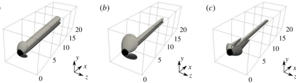
y y x x z z y x z (a) (b) (c) 0 5 10 15 20 0 5 10 15 20 0 5 10 15 20
FIGURE 7. Flow case at Re = 280 for the unstable planar-symmetric base flow.
Three-dimensional view of the mode at (σ, St) = (0.0105, 0.1317). The iso-surfaces of the (a) streamwise, (b) vertical and (c) transverse perturbation velocities are plotted for the levels u0
= ±0.25, v0
= ±0.15 and w0
= ±0.25, respectively. Light and dark grey iso-surfaces for positive and negative perturbation velocities, respectively. The sphere is represented in black.
compact shape than that of the steady mode observed for the regular bifurcation, where its perturbation velocities are almost of the same order.
This symmetry property is further identified through the cross-sections in the x–z and y–z planes reporting the contours of the velocity components (figure 8). In particular, the symmetric solutions of the eigenvalue problem are found to verify: u(x, −y, z) = u(x, y, z), v(x, −y, z) = −v(x, y, z), w(x, −y, z) = w(x, y, z), similar to a varicose instability with respect to symmetry plane associated with the base flow. Figure 8 also shows that the characteristic wavelength of the mode in the streamwise direction varies from λx ≈2Ds inside the bubble to λx≈7Ds in the wake region,
indicating that λx is of the same order as the recirculation length and its phase
velocity increases as it propagates downstream. This gives some further concerns on the inherent difficulty of local stability analysis to provide accurate results for determining critical parameters associated with the Hopf bifurcation (see Pier 2008). Consistently with the shedding of hairpin structures observed in the DNS carried out by Tomboulides & Orszag (2000) and similarly to the stability analysis of Citro et al. (2017), the eigenmode exhibits a wave shape that moves away from the sphere with the same inclination of the recirculation region and more specifically leaving
3 -3 3 -3 0 y y y z 5 10 15 20 3 -30 5 10 15 20 0 5 10 15 x 20 3 -3 0 5 10 15 20 (a) (b) (c) (d)
FIGURE 8. Flow case at Re = 280 for the unstable planar-symmetric base flow.
Cross-sections of the mode at (σ, St) = (0.0105, 0.1317). The contours of the streamwise perturbation velocity are plotted on the (a) x–y and (c) x–z planes for the levels u0
= ±0.25. The contours of the (b) vertical and (d) transverse perturbation velocities are plotted for the levels v0
= ±0.15 and w0
= ±0.25, respectively. Light and dark grey iso-lines for positive and negative perturbation velocities, respectively. The sphere is represented in black.
the region of the maximum shear associated with the transverse direction. This gives further support to the idea that the unstable mode is linked to the linear onset of periodic shedding of hairpin vortices observed both experimentally and numerically by Johnson & Patel (1999) and Szaltys et al. (2012).
The conjugate complex pair of unstable eigenvalues is very isolated but it can be interesting to look at the stable sub-dominant mode at (σ , St) = (−0.06882, 0.1184) found in figure 6(b). Fabre et al. (2008) argues the existence of an anti-symmetric sub-dominant mode that might become temporally amplified for increasing Reynolds numbers. The global sub-dominant mode is visualized by plotting the corresponding streamwise perturbation velocity in figure 9. The eigenmode structure is still planar-symmetric but rotated by 90◦
with respect to the dominant unstable eigenmode and very little differences exist in terms of the streamwise wavelength. This sub-dominant mode moves towards the unstable region for increasing Reynolds number but, for the Reynolds number range considered, the mode remains temporally damped and its evolution is not shown.
4.5. Fixed point versus mean flow stability analysis
To further elucidate the connection between the shedding of hairpin structures and the temporally amplified eigenmode, unsteady nonlinear calculations are carried out for the cases at Re = 280, 300 and 320. The nonlinear calculations are initialized with the steady planar-symmetric base flow solution and allowed to evolve in time until saturation. The time history of a probe located in the sphere wake at Re = 300 is reported in figure 10(a). A 3-D view of the unsteady dynamics is shown in figure 10(b), where the instantaneous iso-surfaces of the Q-criterion at a level of Q = 0.5 show the legs of the shed hairpin vortices at a Strouhal number of St = 0.1345. The observed coherent motion presents strong similarities with both the DNS by Johnson & Patel (1999) and the dye pattern in water experimentally
3 -3 3 -3 0 5 10 15 20 0 5 10 15 20 (b) (a) (c) 0 5 10 15 x x y z y z 20
FIGURE 9. Flow case at Re = 280 for the unstable planar-symmetric base flow. (a)
Three-dimensional view of the iso-surfaces of the streamwise perturbation velocity associated with the mode at (σ , St) = (−0.08682, 0.1184) plotted for the levels u0
= ±0.25. The contours of the streamwise perturbation velocity are plotted on the (b) x–y and (c) x–z planes for the levels u0
= ±0.25. Light and dark grey colours for positive and negative perturbation velocities, respectively. The sphere is represented in black.
-0.018 -0.021 -0.024 -0.027 4000 4050 4100 t u (a) (b) x x x y y z z 4150
FIGURE 10. Unsteady nonlinear calculations at Re = 300: (a) streamwise velocity time
history of the probe located in the sphere wake; (b) three-dimensional view of the unsteady nonlinear calculations. Iso-surfaces of the Q-criterion at a level of Q = 0.5. The zero-streamwise velocity iso-surface in dark grey shows the planar-symmetric separation region behind the sphere (represented in black).
reported by Schouveiler & Provansal (2002) and indicates the temporally amplified mode is responsible for the bifurcation from the double-threaded steady wake with very long streamwise extent to the time-dependent flow characterized by a succession of interconnected vortices behind the sphere.
The important issue concerning the capability of the global linear stability analysis performed on a fixed point solution in correctly predicting the Strouhal number of the shedding frequency is here addressed. For a 2-D cylinder flow, Barkley (2006) shows that while linear stability on the mean flow correctly captures the shedding frequency, when the stability is performed on the fixed point solution the predicted
Re LFP sep L MF sep (σ , St) FP (σ, St)MF StNL 280 1.43 1.42 (0.0105, 0.1317) (≈0.000, 0.1323) 0.1325 300 1.48 1.36 (0.0704, 0.1324) (≈0.000, 0.1347) 0.1345 320 1.51 1.32 (0.0955, 0.1442) (≈0.000, 0.1482) 0.1483
TABLE 2. Comparisons between global linear stability analysis carried out on the fixed point (FP) and mean flow (MF). The Strouhal number of the nonlinear DNS calculations (StNL
) is also reported.
Parameters Sphere flow
Free-stream Mach number M ∈ [0.3; 1.2]
Free-stream stagnation temperature Ti,∞=287 K
Free-stream stagnation pressure Pi,∞=1.013 × 10⁵ Pa
Reynolds number Re ∈ [210; 370]
TABLE 3. Free-stream parameters for the bifurcation Mach evolution analysis.
frequency rapidly diverges with the Reynolds number once past the bifurcation. The same analysis can be done by performing the stability analysis on the mean flows calculated over 32 snapshots taken during one period at saturation for the aforementioned cases. Table2 reports the separation length and eigenvalues calculated by performing global linear stability on the fixed point (FP) and mean flow (MF) solutions. The Strouhal number associated with the nonlinear DNS calculations (StNL)
is also reported. Since the mean flow is viewed as a marginally stable solution when considered as a steady solution, the growth rate predicted by the linear stability is about zero and no further information can be extracted. As seen for the 2-D cylinder case, the global stability analysis performed around the mean flow better predicts the shedding frequency of the nonlinear DNS calculations. However, it is interesting to see that the shedding frequencies predicted by the stability analysis on fixed point and mean flow do not diverge as quickly. For the same 1Re = 40 above the supercritical bifurcation Reynolds value, this difference is approximately 25 % for the 2-D cylinder and approximately 3 % for the sphere.
5. Mach evolution of the regular and Hopf bifurcations
Extending the work of Meliga et al. (2010) with the objective of explaining the study of Nagata et al. (2016,2018), the evolution of the regular and Hopf bifurcations with Mach and Reynolds number is tracked. A fully 3-D global stability analysis is performed for each case investigated to follow the bifurcations and explain the appearance, or better the disappearance, of temporally amplified global modes. Low Reynolds number and low-supersonic cases are selected (see table 3) and the same analysis carried out for the nearly incompressible study is repeated.
5.1. Simulation details
While for all the subsonic cases up to M = 0.75 the numerical set-up used for the nearly incompressible analysis is unchanged, for the M = 0.9 and supersonic cases a different domain configuration is selected and reported in figure11. The computational domain is composed of 6 blocks in an ellipsoidal configuration to better follow the
x (a) (b) x y y z 30 D s 10 Ds 30 Ds
FIGURE 11. Three-dimensional (a) and lateral (b) views of the numerical domain for the
M =0.9 and supersonic flow cases.
bow shock that forms in front of the sphere. Although adapted to the new domain configuration, the same boundary conditions for the nearly incompressible case are used for both fixed point and linear stability calculations (see §§3.1 and 3.2, respectively). To confirm the grid capability to reproduce the correct physics, the nearly incompressible case at Re = 280 is repeated on the new domain configuration and good agreement with the previous numerical set-up is obtained. Furthermore, the base flow at Re = 300 and M = 1.2 is also compared with the numerical results by Nagata et al. (2016) and good match in terms of shock shape and shock stand-off distance is achieved. The chosen grid resolution is (nx, ny, nz) = (224 × 112 × 112)
for each block.
5.2. Base flow Mach evolution
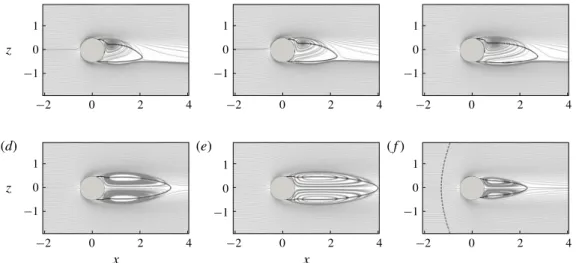
As shown by Nagata et al. (2016, 2018) in their nonlinear unsteady calculations, the large-scale effect of the increasing Mach number on the base flow is to cause the axisymmetrization of the separated region behind the sphere. Table 4 reports separation lengths and information on the base flow symmetry characteristics, whether it is axisymmetric (AS) or planar-symmetric (PS), for each case investigated. The symbol ‘×’ is used to indicate the cases that have not been analysed. For the case at Re = 280, the base flow Mach evolution is shown in figure 12 by the projections of the 3-D streamlines on the x–z plane for the cases at (a) M = 0.1, (b) M = 0.3, (c) M = 0.6, (d) M = 0.75, (e) M = 0.9 and ( f ) M = 1.2. The solid black lines indicate the separation region by plotting the contours of the zero-streamwise velocity. The presence of the bow shock in front of the sphere is highlighted by the dashed black line, upstream of which the flow is undisturbed and the streamlines are parallel to the x-axis. In the subsonic regime, when the same configuration of azimuthal symmetry is kept the effect of the Mach number on the base flow is the same as that of the Reynolds number and the size of the separation region increases with the Mach number (figure 12a–c). When a change from planar to axisymmetry occurs for increasing Mach number and fixed Reynolds number (figure 12c,d) the separated region ‘bursts’ into a much larger one. It is important to specify that for all these cases the flow is everywhere subsonic and no shocks are formed either in front or on the sphere. On the contrary, particular attention needs to be given to the base flow of the supersonic cases, for which a bow shock is formed. When passing from subsonic
1 0 -1 1 0 -1 1 0 -1 1 0 -1 1 0 -1 1 0 -1 -2 0 2 x z z (d) (e) (f) x 4 -2 0 2 4 -2 0 2 4 -2 0 2 4 -2 0 2 4 -2 0 2 4
FIGURE 12. Base flow Mach evolution at Re = 280. Three-dimensional streamlines
projected onto the x–z plane for the (a) M = 0.1, (b) M = 0.3, (c) M = 0.6, (d) M = 0.75, (e) M = 0.9 and ( f ) M = 1.2 cases. The separated region is indicated by the solid black line. For the supersonic case, the shock is represented by the dashed black line.
6 (a) (b) 4 4 2 0 0 5 10 x 0 2 -2 -4 2 2 4 0 z y y x 1 0 5 10 15
FIGURE 13. Schlieren-like visualization of the base flow at Re = 280 and M = 1.2.
Contours of the density gradient on (a) the two perpendicular x–y and x–z planes and (b) a 2-D view on the x–y plane.
to supersonic flow conditions, either if the azimuthal symmetry changes or not, the separated region behind the sphere becomes significantly shorter (figure 12e, f ). However, also for the supersonic case at M = 1.2, the effect of the Reynolds number on the separation length is the same as in the subsonic case and the separated region increases in size with the Reynolds number (see the column at M = 1.2 in the table4). Figure 13 shows the contours of the density gradients in a 3-D view in (a) the two perpendicular x–y and x–z planes and (b) in a 2-D view of the x–y plane. The bow shock that forms in front of the sphere forces the axisymmetry of the separated region behind the sphere. The Schlieren-like contours also show the expansion fans that generate on the sphere and diverge while moving downstream. These obtained base flows are used to perform global stability analysis and investigate the evolution of the regular and Hopf unstable bifurcations.
0 0.5 1.0 −0.04 −0.02 0 ß M St 0.02 (a) (b) 0 0.5 1.0 0 0.05 0.10
FIGURE 14. Hopf bifurcation. Mach evolution of the (a) temporal amplification rate and
(b) Strouhal number for the least temporally damped/most temporally amplified oscillatory global mode at Re = 280.
Re M =0.1 M =0.3 M =0.6 M =0.75 M =0.9 M =1.2
200 1.36 (AS) × × × × ×
210 1.39 (AS) 1.54 (AS) 1.96 (AS) × × ×
220 1.42 (AS) 1.58 (AS) 2.00 (AS) × 3.11 (AS) ×
250 1.49 (AS) 1.67 (AS) 2.15 (AS) × 3.32 (AS) 1.64 (AS)
260 1.51 (AS) × × × × ×
270 1.39 (PS) × × × × ×
280 1.43 (PS) 1.63 (PS) 2.09 (PS) 2.79 (AS) 3.50 (AS) 1.81 (AS)
290 1.46 (PS) × × × × ×
300 1.48 (PS) 1.68 (PS) 2.16 (PS) × 3.62 (AS) 1.91 (AS)
320 1.51 (PS) 1.72 (PS) 2.22 (PS) × 3.60 (PS) 2.00 (AS)
345 × × × × 3.69 (PS) 2.11 (AS)
370 × × × × 3.79 (PS) 2.21 (AS)
TABLE 4. Reynolds and Mach number base flow separation lengths and symmetry characteristics (AS = axisymmetric, PS = planar-symmetric) evolution.
5.3. Bifurcation Mach evolution
The Hopf bifurcation is first analysed for Re = 280. The Mach evolution of the most temporally amplified global mode is reported in figure 14 in terms of (a) growth rate and (b) Strouhal number. Despite some differences with the findings of Meliga et al. (2010) that may be well due to either their base flow axisymmetry hypothesis or the constant molecular viscosity and thermal conductivity assumption, the present results confirm that the Mach number initially shows a destabilizing effect on the sphere wake and the growth rate of the global mode increases for M = 0.3. However, when the Mach number is further increased the global mode is damped and its growth rate that still has a positive sign at M = 0.6 becomes negative at M = 0.75, individuating the threshold of the Hopf bifurcation. Similarly to what found by Nagata et al. (2016,
2018), accordingly with the increasing size of the separation, the frequency of the most temporally amplified mode decreases with the Mach number. It is interesting to see that at M = 0.75 the axisymmetric base flow is unstable and a temporally amplified non-oscillatory mode appears, as shown in figure 15(a).
ß (a) (b) −0.2 −0.3 −0.1 0 0.3 0.3 St St 0.1 0.2 −0.05 0 0.05 −0.2 −0.3 −0.1 0 0.1 0.2 −0.60 −0.40 −0.20 0
FIGURE 15. Eigenspectra in the St–σ plane for the cases at Re = 280 and (a) M =
0.75 and (b) M = 1.2. The axisymmetric base flows shown in figure 12(d, f ) are used, respectively. 0 (a) (b) (c) 5 x y z x y z x y z 1015 20 0 5 10 1520 0 5 1015 20
FIGURE 16. Flow case at Re = 280 and M = 0.75 for the unstable axisymmetric base
flow. Three-dimensional view of the iso-surfaces of the (a) streamwise, (b) radial and (c) azimuthal perturbation velocities associated with the mode at (σ , St) = (0.04799, 0.0) plotted for the levels v0
x= ±0.10, v 0
r= ±0.03 and v 0
θ= ±0.03, respectively.
Similarly to what done for the incompressible modes around the first bifurcation, a transformation of coordinates (from Cartesian to cylindrical) has been applied to transform the streamwise, vertical and transversal (u0, v0, w0) perturbation velocities
into streamwise, radial and azimuthal (v0 x, v
0 r, v
0
θ) ones. The iso-surfaces of the
perturbation velocities associated with the mode at (σ , St) = (0.04799, 0.0) reported in figure 16 show the resemblance to the temporally amplified non-oscillatory mode found in the nearly incompressible analysis, i.e. at Re = 210 (see figure 5), that similarly causes the loss of axisymmetry due to an azimuthal mode with wavenumber m =1. When the Mach number is further increased up to M = 1.2, the axisymmetric base flow solution becomes stable, identifying the threshold of the regular bifurcation. Figure 15(b) shows the eigenspectrum for the globally stable axisymmetric base flow at M = 1.2 and the corresponding iso-surfaces of the perturbation velocities (streamwise, radial and azimuthal) associated with the non-oscillatory mode at (σ , St) = (−0.0101, 0.0) are reported in figure 17. The presence of the bow shock and the consequent expansion fans on the sphere cause the appearance of a structure attached to the sphere. Although the base flow solution is stable and this mode is not temporally amplified, the azimuthal character of the eigenfunction is still associated with an azimuthal wavenumber m = 1. The same analysis is repeated for all the considered Reynolds and Mach numbers and the most temporally amplified/least
0 (a) (b) (c) 5 x y z x y z x y z 10 1520 0 5 1015 20 0 5 10 1520
FIGURE 17. Flow case at Re = 280 and M = 1.2 for the stable axisymmetric base
flow. Three-dimensional view of the iso-surfaces of the (a) streamwise, (b) radial and (c) azimuthal perturbation velocities associated with the unstable mode at (σ , St) = (−0.0101, 0.0) plotted for the levels v0
x = ±0.02, v 0 r = ±0.005 and v 0 θ = ±0.005, respectively.
temporally damped modes are presented in table 5. Thus, it is possible to draw a stability map and follow the boundaries of the two bifurcations, as shown in figure 18. Stable axisymmetric base flows (dark grey region) are indicated by full circle symbols. Unstable axisymmetric base flows (light grey region) characterized by a temporally amplified non-oscillatory planar-symmetric mode are represented as empty circles. The empty triangle symbols correspond to unstable planar-symmetric base flows (white region) characterized by a temporally amplified oscillatory planar-symmetric mode. Two unexplored regions are indicated and framed by dash-dotted lines: a first one at low-Mach/high-Reynolds numbers, where an unsteady periodic base flow exists and a Floquet’s analysis would be necessary, and a second one in the transonic region where the shock would be attached to the sphere. Although the physics might significantly change in the latter, due to the low Reynolds number range under consideration this second unexplored region is expected to be very narrow (Nagata et al. 2016).
For increasing values of the Mach number, the regular and Hopf bifurcations seem to move towards higher values of Reynolds numbers. However, for a sufficiently high Reynolds number (i.e. for approximately Re> 345) and if the narrow transonic region not examined is ignored, only a supercritical Hopf bifurcation exists and for increasing Mach number the base flow solution directly passes from an unstable planar-symmetric configuration characterized by temporally amplified oscillatory modes to a stable axisymmetric one, as seen by Nagata et al. (2016).
5.4. Convective instabilities
Figure 18 shows that, for the examined range of Reynolds numbers, the supersonic flow configurations are globally stable. The system is no longer a self-sustained oscillator and switches to a noise-amplifier type. To characterize the convective nature of the system, the case at (Re, M) = (370, 1.2) is selected, being the expected most convectively unstable one. The corresponding eigenspectrum is shown in figure 19(a), for positive Strouhal values only. As visible from figure 15(b) for the case at (Re, M) = (280, 1.2), the continuous branch does not change and the two modes at (σ , St) = (−0.405, 0.135) and (σ , St) = (−0.393, 0.167) move away and reach (σ , St) = (−0.3106, 0.1268) and (σ , St) = (−0.378, 0.166). The inset in figure 19(a) shows the evolution of these two modes in the Reynolds number range investigated at M = 1.2. In qualitative agreement with Nagata et al. (2018), if a linear trend with the Reynolds number is assumed these two modes would become globally unstable
0 0.3 0.6 0.9 1.2 200 220 240 260 280 Re M 300 320 340 360 380 Unexplored Unexplored
FIGURE 18. Evolution of the regular and supercritical Hopf bifurcations with the Mach
and Reynolds numbers. The coloured regions represent stable axisymmetric base flow solutions (dark grey region and full circle symbols), unstable axisymmetric base flow solutions characterized by temporally amplified non-oscillatory planar-symmetric modes (light grey region and empty circle symbols) and unstable planar-symmetric base flow solutions characterized by temporally amplified oscillatory planar-symmetric modes (white region and empty triangle symbols).
Re M =0.1 M =0.3 M =0.6 M =0.75 M =0.9 M =1.2 200(−1.432 × 10⁻³, 0.0) × × × × × 210 (0.683 × 10⁻³, 0.0) (−0.008, 0.0) (−0.027, 0.0) × × × 220 (2.615 × 10⁻³, 0.0) (0.152, 0.0) (0.031, 0.0) × (−0.034, 0.0) × 250 (0.008, 0.0) (0.815, 0.0) (0.418, 0.0) × (0.005, 0.0) (−0.094, 0.0) 260 (0.009, 0.0) × × × × × 270 (−0.212, 1.318) × × × × × 280 (0.105, 1.317) (0.236, 1.251) (0.106, 1.129) (0.480, 0.0) (0.006, 0.0) (−0.102, 0.0) 290 (0.412, 1.321) × × × × × 300 (0.704, 1.324) (0.871, 1.257) (0.642, 1.148) × (0.007, 0.0) (−0.107, 0.0) 320 (0.955, 1.442) (1.806, 1.228) (1.122, 1.151) × (−0.009, 0.0) (−0.113, 0.0) 345 × × × × (0.226, 0.868) (−0.119, 0.0) 370 × × × × (0.570, 0.862) (−0.126, 0.0)
TABLE 5. Growth rate (σ) and Strouhal number (St), Reynolds and Mach number evolution of the most temporally amplified/least temporally damped eigenvalue. Both growth rate and Strouhal numbers have been multiplied by 10.
for a Reynolds number range of Re = 1000 ± 300. These two modes have a very similar spatial distribution and, only for the mode at (σ, St) = (−0.378, 0.166), the contours of the streamwise, normal and transversal perturbation velocities are plotted in figures 19(b), 19(c) and 19(d), respectively.
To study the convectively unstable character of the flow case at(Re, M) = (370, 1.2), an unsteady nonlinear simulation has been carried out by restarting the calculation from the axisymmetric base flow solution presented in §5.2 (figure 12f) and applying a Gaussian random white noise forcing. The white noise forcing is introduced
0 0 0.1 0.2 St ß (a) (b) (c) (d) 0.3 -0.20 -0.30 2 -2 0 5 10 15 0 5 10 15 0 10 x y y y 15 2 -2 2 -2 Re Re 0.16 0.14 -0.35 -0.40 -0.40 -0.60
FIGURE 19. (a) Eigenspectrum in the St–σ plane for the case at (Re, M) = (370, 1.2).
The inset shows the Reynolds evolution of the two modes leaving the continuous branch. For the mode at (σ , St) = (−0.378, 0.166), the contours of the (b) streamwise, (c) vertical and (d) transversal perturbation velocities are plotted for the levels u0
= ±0.03, v0
= ±0.01 and w0
= ±0.01, respectively.
upstream of the bow shock that forms in front of the sphere according to
u(x, y, z, t) = Aoexp " −(x − xf) 2 2σ2 x −(y − yf) 2 2σ2 y −(z − zf) 2 2σ2 z # W(x, y, z, t). (5.1) The forcing is applied continuously and localized spatially by a Gaussian function centred in (xf, yf, zf) = (−5, 0, 0). The variances associated with the spatial Gaussian
distributions in the three spatial directions (σx, σy, σz) are adjusted to have a 3-D
ellipsoid that approximately extends (2, 3, 3) × Ds in the streamwise, vertical and
transversal directions, respectively. The applied perturbation amplitude Ao corresponds
to a turbulent intensity, measured as the ratio between the root-mean-square (r.m.s.) value of the streamwise perturbation velocity and its mean value at the centre of the forcing region, of Tu ≈ 0.1 %. The numerical white noise W(x, y, z, t) varies in the range [−0.5, 0.5] around the zero mean and it varies for each spatial point and each time iteration. The forcing is ramped up to full strength after about an eighth of a flow-through time. Numerical artefacts, such as grid resolution and time-step size, limit the frequency band of the dynamic response above St = 1. Therefore, the plots have been cut at this value above which the response for the present analysis is not relevant.
The time response of the system is monitored by six probes located on the streamwise axis at different x-locations and four ones located on the circular separation line in the downstream half of the sphere and azimuthally separated every 90◦
. Since the results show an azimuthally independent behaviour, only the probes along the streamwise axis are here presented. Figure 20 shows the location of the six probes considered, the bow shock location and the spatial distribution of the applied random forcing. After an initial transient, the time histories are recorded for approximately 16 flow-through times and a Fourier analysis is performed. The power spectral density (PSD) distribution as a function of the Strouhal number is
Forcing region
1 2 3 4 5 6
Shock
FIGURE 20. Spatial distribution of the probes used to monitor the time response of the
system. Probe 1: (x, y, z) = (−2.0, 0.0, 0.0); probe 2: (x, y, z) = (−0.7, 0.0, 0.0); probe 3: (x, y, z) = (1.0, 0.0, 0.0); probe 4: (x, y, z) = (2.0, 0.0, 0.0); probe 5: (x, y, z) = (4.0, 0.0, 0.0); probe 6: (x, y, z) = (8.0, 0.0, 0.0). 10-2 10-4 10-6 10-8 10-2 10-4 10-6 10-8 10-2 10-4 10-6 10-8 10-2 10-4 10-6 10-8 10-2 10-4 10-6 10-8 10-2 10-4 10-6 10-8 10-2 10-1 100 10-2 10-1 100 10-2 10-1 100 10-2 10-1 St St PSD PSD (a) (b) (c) (d) (e) (f) St 100 10-2 10-1 100 10-2 10-1 100
FIGURE 21. Fourier analysis performed on the time histories recorded on the monitoring
probes (probe 1 – a; probe 2 – b; probe 3 – c; probe 4 – d; probe 5 – e; probe 6 – f ). Power spectral density as a function of the Strouhal number.
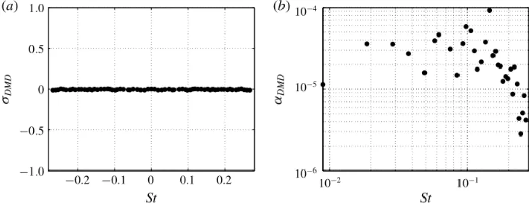
plotted in figure 21 for the monitored probes. The perturbation reaches the shock and maintains its white noise features (probe 1, figure 21a). The bow shock acts like a low-pass filter, cutting all the frequencies above St ≈ 0.5 and reducing the energy of approximately one order of magnitude (probe 2, figure 21b). The sphere then selects a frequency at a Strouhal number of St ≈ 0.15 and a peak appears (probe 2, figure 21c). The energy associated with this peak increases in the downstream probes (probe 4 to 6, figure 21e–f ) and eventually saturates. However, the energy associated with the perturbations downstream of the sphere is low, the complete flow field conserves its axisymmetric characteristics and no evidence of transition in the wake exists. A dynamic mode decomposition (DMD) (Schmid 2010) is performed by taking 256 nonlinear snapshots during the same time interval used to record the probe time
1.0 10-4 10-5 10-6 10-2 10-1 0.5 0 ßDMD åDMD -0.5 -1.0 (a) (b) -0.2 -0.1 0 St 0.1 0.2 St
FIGURE 22. DMD analysis: (a) growth rate and (b) amplitude of the DMD modes as
a function of the Strouhal number. The contribution of the mean flow is not taken into account.
histories for the Fourier analysis. The ‘amplitude’ (αDMD) associated with each DMD
mode is computed by projecting each mode on the first snapshot (Jovanovic, Schmid & Nichols 2014). To avoid to compromise the DMD mode amplitude calculations, the analysis is performed only on a subspace of the numerical domain that excludes the region where the white noise forcing is applied. The DMD growth rate (σDMD) and
amplitudes are reported in figure 22 as a function of the Strouhal number. Since the snapshots are taken in the limit cycle, the associated DMD growth rates are nearly zero (figure 22a). However, the distribution of DMD amplitudes in figure 22(b) shows that not all modes contribute in the same way as the system dynamics. If the contribution of the mean flow (that obviously is the highest one) is not taken into account, the DMD amplitude distribution not only resembles the PSD distributions in the sphere wake but it also shows that the highest contribution is given by the mode at a Strouhal number of St = 0.145 that closely matches the peak Strouhal number found in figure 21(c–f ). It can be interesting to compare the perturbation velocity fields, from which the mean flow is subtracted, with the DMD mode velocities. Figure 23 reports the contours of the streamwise (a,b), vertical (c,d) and transversal (e, f ) velocities on a longitudinal slice in the x–y plane for the perturbation field (a,c,e) and DMD mode at St = 0.145 (b,d,f ). While the near-wake region in the perturbation field is affected by the white noise forcing and no appropriate comparison can be made, for x> 5 it is possible to appreciate that perturbation velocity field and DMD eigenmode velocities have a similar structure. This confirms that the DMD mode at St =0.145 is well capturing the perturbations dynamics. It is also interesting to see that the shape of the DMD mode strongly relates to what seen for the globally stable mode shown in figure 19(b–d) at a similar Strouhal number, suggesting a response of the system that is still very modal. Some similarities can be found between this mode and that found at (Re, M) = (280, 0.1), especially in terms of shape and wavelength of the streamwise and transversal perturbation velocities (compare figures 8c,d with figures 23b, f ). This might indicate that the response of the system to a sufficiently strong forcing or at higher Reynolds number could lead to the shedding of hairpin vortices from the sphere wake, like in the incompressible counterpart. To support this idea, the work by Nagata et al. (2018) shows that unsteady hairpin shedding happens at (Re, M) = (1000, 1.2). To verify the convective nature of the flow and its global stability, the white noise forcing is switched off and the total energy fluctuations
2 (a) (b) (c) (d) (e) (f) y -2 2 y -2 2 y -2 2 -2 2 -2 2 -2 0 5 10 15 0 5 10 15 0 10 x 15 0 5 10 15 0 5 10 15 0 10 x 15
FIGURE 23. Comparison between the perturbation field (a,c,e) and DMD eigenmode at
St =0.145 (b,d,f ). Streamwise (a,b), vertical (c,d) and transverse (e,f ) velocities.
time histories recorded by the probes in the sphere wake are reported in a t–x plot in figure 24. The time at which the forcing is switched off is indicated by a grey dashed line. It is possible to see that a packet of perturbations is convected downstream and damped in time. The total energy fluctuations go to zero and the base flow solution, from which the nonlinear calculation was restarted, is recovered.
6. Conclusions
The effect of compressibility on the global stability of a sphere flow has been investigated. The work by Meliga et al. (2010) is extended up to a low-supersonic regime taking into account of the three-dimensionality of the steady fixed point solutions around the supercritical Hopf bifurcation and the presence of shocks.
The linear dynamics is first analysed at nearly incompressible conditions and the regular and supercritical Hopf bifurcations are described. The three-dimensionality of the fixed point solutions used to study the Hopf bifurcation is found to not have a significant impact on the identification of the instability threshold or on the Strouhal number of the leading mode. However, the spatial structure of the eigenmode perturbations is deflected accordingly to the planar-symmetric sphere wake, consistently with the investigations by Citro et al. (2017) in the incompressible regime. This indicates the importance of removing the axisymmetric flow assumptions adopted in most of the previous studies and the need to consider fully 3-D fixed point solutions. The question concerning the correctness of the predicted shedding frequency by linear stability performed on a fixed point solution is also addressed. When the linear stability analysis is performed on the mean flow for some cases above the supercritical Hopf bifurcation, the predicted shedding frequency closely matches the nonlinear one. Although the shedding frequencies predicted by the global stability analysis on fixed point and mean flow solutions do not diverge for increasing Reynolds number above the bifurcation threshold as fast as seen for the two-dimensional cylinder case (Barkley 2006), it is important to consider this aspect depending on the type of analysis intended. When the identification of the bifurcation threshold (or in general the stability of the flow) is not needed, a global
8 6 6 5 4 3 2 1 Shock 4 2 0 -2 6.91 6.92 (÷104) t x
FIGURE 24. Total energy fluctuations time histories in a t–x plot. The time at which the
forcing is switched off is indicated by the vertical grey dashed line. The sphere, shock and probe locations are sketched on the right-hand side.
stability analysis performed on the mean flow solution as a base flow might be more appropriate for establishing the frequencies associated with the nonlinear dynamics.
To explain the observations of the nonlinear DNS calculations of Nagata et al. (2016, 2018), the bifurcation boundaries are followed in a Re–M space. In agreement with the work of Meliga et al. (2010), an initial destabilizing effect of the Mach number is found around the supercritical Hopf bifurcation. However, when the Mach number is further increased to supersonic speeds, it is possible to conclude that the Mach number has a stabilizing effect on the global behaviour of the flow and the thresholds of the two bifurcations move towards higher Reynolds numbers. For sufficiently high Reynolds numbers, when the Mach number is increased the solution directly passes from an unsteady planar-symmetric solution to a steady axisymmetric one for supersonic speeds.
At supersonic conditions, the flow becomes globally stable and the system switches from an oscillator to a noise amplifier. A forced nonlinear calculation is carried out to characterize the convective nature of the flow and the performed Fourier and DMD analyses indicate that a link with the incompressible dynamics above the incompressible Hopf bifurcation might exist. This is partially supported by the nonlinear DNS calculations by Nagata et al. (2018), who show that the transition to an unsteady wake at supersonic speeds happens via hairpin vortices shedding when the Reynolds number is significantly increased. A definite confirmation would come by global stability calculations at higher Reynolds numbers and a continuation of this work shall be therefore focused on the study of cases in this regime. Another continuation of this work could interest cases at higher Mach numbers, where the flow dynamics might change due to a bow shock that gets closer to the sphere.
Although limited to laminar flow cases, the present work represents a necessary preliminary step towards the study of the turbulent regime, for which large-scale coherent motions persist. In the nearly incompressible limit, Taneda (1978) shows that the turbulent wake of a sphere exhibits a wave-like motion similar to the one observed in the laminar case. By adding an artificial viscosity to account for the turbulent small scales, a linear stability analysis carried out on the mean flow