Science Arts & Métiers (SAM)
is an open access repository that collects the work of Arts et Métiers Institute of
Technology researchers and makes it freely available over the web where possible.
This is an author-deposited version published in: https://sam.ensam.eu Handle ID: .http://hdl.handle.net/10985/8768
To cite this version :
Laurent GUILLON, Charles HOLLAND, Christopher BARBER - Cross-Spectral Analysis of Midfrequency Acoustic Waves Reflected by the Seafloor IEEE Journal of Oceanic Engineering -Vol. 36, n°2, p.248-258 - 2011
Any correspondence concerning this service should be sent to the repository Administrator : archiveouverte@ensam.eu
Cross-Spectral Analysis of Midfrequency Acoustic Waves
Reflected by the Seafloor
Laurent Guillon, Charles W. Holland, and Christopher Barber, Member, IEEE
Abstract—Direct path measurements of a single-bottom
inter-acting path on a vertical array are used to probe the seabed struc-ture. The phase of the cross-spectrum, commonly used in engi-neering acoustics, permits examination of the importance of sub-bottom paths. When the cross-spectral phase is linear with fre-quency it implies that source to receiver propagation is dominated by a single path. A linear cross-spectral phase would also satisfy the linear seabed reflection coefficient phase approximation some-times employed in forward modeling and geoacoustic inversion approaches. Shallow water measurements of the cross-spectrum, however, evidence a strongly nonlinear phase, below about 1500 Hz at one site, and 600 Hz at another site, implying that: 1) the sub-bottom structure plays an important role (i.e., a seabed half-space approximation would be inappropriate); and 2) the linear reflec-tion phase approximareflec-tion would be violated at those frequencies.
Index Terms—Acoustic reflection, cross-spectrum, sediments,
underwater acoustics.
I. INTRODUCTION
A
COMMON assumption in long-range acoustic modeling and geoacoustic inversion is that the seabed can be treated as a half-space. While it is usually possible to fit seabed param-eters to propagation data using the half-space approximation, the fits do not provide compelling evidence that the underlying assumption is correct (or equivalently that the estimated param-eters represent true physical properties).In this paper, we use cross-spectral analysis for a single-bottom interacting path in order to gain insight into the importance of seabed layering on long-range propagation. This is done using both measured and synthetic cross-spectra at low-grazing angles. High-grazing angles are also examined.
When the phase of the cross-spectrum is linear, it indicates a single-path regime, i.e., seabed interaction is dominated by a single boundary. At first blush, a linear phase might suggest that a half-space approximation is correct, or equivalently that the
Associate Editor: R. Chapman.
L. Guillon is with the Research Institute, French Naval Academy, 29240 Brest, Cedex 9, France (e-mail: laurent.guillon@ecole-navale.fr).
C. W. Holland and C. Barber are with the Applied Research Laboratory, Penn-sylvania State University, State College, PA 16804 USA. (e-mail: cwh10@psu. edu; cbarber@psu.edu)
single-path is the path reflecting off the water-sediment inter-face. However, this may or may not be the case. For example, when a soft sediment layer (i.e., sediment sound speed is less than that in seawater) overlies a harder sediment, a linear phase (single-path regime) could occur where the dominant path re-fracts through the upper soft layer and is reflected off the hard sediment. This could happen at both steep and low angles (slow sediments exhibit no critical angle). The phase could be linear in this case over particular frequency ranges, punctuated by non-linear phase shifts at nearly regularly spaced frequencies (which may or may not be observable depending on the available band-width). Thus, we can conclude that when the phase is nonlinear, layering is important, and when the phase is linear, layering may or may not be important.
Estimates of the cross-spectral phase also permit examination of the assumption of a linear reflection phase that is used in for-ward modeling and inversion. Within the context of modal de-scription of sound in shallow water area, it has been shown that only the low order modes corresponding to small grazing angles can propagate at long range [1] and these modes interact only with the surficial layers. These observations led to the concept of effective depth (see, e.g., [2] and references therein) which provided accurate predictions of sound field. More recently, P. Joseph [3] has developed a technique to predict shallow water propagation and to characterize the seafloor based on the same observation of a linear relation between the reflection phase and the vertical component of the acoustic wave number at the seabed. In this context, the measurement of the phase of cross-spectra could be useful because it gives information on the low frequency limit where this linearization of the reflection phase can be applied. If the linear reflection phase is a good assump-tion, the cross-spectral phase will be linear.
The starting point of the present paper is an experimental configuration used to establish a joint time-frequency inver-sion method [4], [5]: an omnidirectionnal broadband signal is emitted by a source near the surface and the reflected signal is recorded on a vertical array. The data obtained with this ex-perimental conguration were also used recently to check a new geoacoustic inversion method based on image sources [6]. In a previous paper [7], we have shown that the cross-correlation of received signals between vertically separated hydrophones is very sensitive to the geoacoustic composition of the seafloor. The large band of the signal (roughly 100 Hz–6 kHz) leads to a large range of wavelengths: from 25 cm to 15 m. The inter-action between an acoustic wave and a layered seafloor being greatly dependent on the wavelength, a study of the correlations
TABLE I
DISTANCESBETWEEN THEHYDROPHONES OF THEVERTICALARRAY
Fig. 1. Sketch of the experiment. Hydrophone number 1 is the closest from the seafloor. The distance between the source and the seafloor is . The reflected acoustic geometric path between the source and first hydrophone is at grazing angle.
along the array in the frequency domain is necessary. That is the main contribution of the present paper which focuses on the cross-spectrum of the signals.
The paper is organized as follows. In Section II, the at-sea data are described. Then, in Section III, the cross-spectrum is defined and its properties are described. We also present a nu-merical model based on the Sommerfeld integral that allows us to obtain synthetic data. In Section IV, the influence of noise on the cross-spectrum analysis is detailed. In Section V, the mea-surements and the simulations are compared. Finally, results are summarized and discussed in Section VI.
II. DESCRIPTION OF THEDATA
A. Experimental Data
The data were obtained during scattering and reverberation from the sea bottom (SCARAB) 97 campaign conducted by the NATO Undersea Research Center (NURC), La Spezia, Italy, in June 1997 in Capraia basin area in the northern Tyrrhenian Sea. Here, we focus on data from two sites at (10.1088 E, 43.08558 N), and (10.0250 E, 43.0145 N), denominated as Site 2 and Site 3, respectively.
The geometry of the experiment employs a fixed vertical array receiver and a towed broadband source (see Fig. 1). The receiver consisted of 16 Benthos AQ-4 hydrophones spaced irregularly over a 62 m aperture. The data were sampled at 24 kHz and low pass filtered at 8 kHz with a seven-pole six-zero elliptic (70 dB per octave roll off) antialias filter. A high-speed digital link within the array provided programmable signal conditioning, digitization, and serialization of the signals. Nonacoustic data (gains, filter settings, etc.) were interleaved in the serial stream and telemetered to the NATO research vessel (NRV) alliance.
TABLE II
GRAZINGANGLES ONFIRST ANDLAST HYDROPHONE OF THE ARRAY FOR THETWOSITES AND THETWODISTANCES
Fig. 2. Sound speed profiles obtained by geoacoustic inversion for Site 2 and 3 (from [5]). Vertical scales are different by factor of ten.
The first hydrophone is 11.5 m above the seafloor in the two sites. The distances between hydrophones are given on Table I. The distance between the source and the receivers array is con-tinuously changing. We have chosen to treat the signals at long and short range, these ranges being different for the two sites because the water depth is different: 150 m for Site 2 and 104 m for Site 3. These two ranges are chosen to have similar grazing angles in both cases (see Table II). Note that these angles are evaluated with the hypothesis of an isovelocity water column.
In this shallow water configuration, signals corresponding to multiple reflected paths are recorded at each hydrophone. Here we are only interested in the first bottom-reflected path which is composed of numerous reflections from the buried interfaces. The time series are windowed to process only this path. When the source–receiver range becomes too large, the various paths merge together. The long ranges indicated in Table II are the longest possible for multipath separation.
One major difference with previous studies [8], [9] is that we can not average results over multiple realizations for three rea-sons. First, since the source is towed, the geometry is different from one realization to another. Second, the source is not per-fectly repeatable. Third, an elegant way to obtain geoacoustic of range-dependent seafloors is to use a source and a horizontal array, these elements being towed by a vessel or an AUV [10], [11]. In this configuration, each ping is a unique realization of the acoustic field between the source and the receiver. Thus, the experimental results presented are the results of a single real-ization which has some important consequences discussed in Section IV.
Fig. 3. Signal emitted by the source (left) in time domain, and (right) in fre-quency domain (normalized autospectrum in decibels). The signal is recorded on one array hydrophone.
B. Geoacoustic Parameters
The geoacoustic parameters at Site 2 and 3 were obtained by analysis and inversion of broad band reflection data using a joint time-frequency technique developed by Holland and Osler [4]. We think that the parameters used here (see Fig. 2) are reason-able estimates of the geoacoustic properties, supported by phys-ical measurements on cores, even if there is no quantitative es-timation of their uncertainty.
Site 2 is in 150 m water depth, with a flat and featureless seabed (from sidescan sonar data), bottom slopes are less than about 0.3 degree. The sound speed and densitie profiles are com-posed of a silty-clay fabric with intercalating sandy sediments (Fig. 2 left). This layering structure is believed to have been cre-ated by high-frequency glacioeustatic sea-level changes during the Pleistocene era.
Site 3 is located on the Elba Ridge in 104 m water depth, separated from Site 2 by the Elba submarine valley which acts a sink for the fine-grained sediment deposited from mainland Italy (Cecina River). The Elba Ridge is of magmatic origins overlain by relatively coarse-grained sediments. Geoacoustic inversion of reflection data from this site [5] are shown in Fig. 2 right.
Besides the difference in sediment fabrics, the basement (from an acoustic point of view, i.e., related to penetration depth of sonar signals) is at subbottom depths greater than 150 m for Site 2 and at 15 m for Site 3.
C. Source Signal
The source was a marine seismic Uniboom which had de-sirable qualities of a short pulse length and broad bandwidth (100–6000 Hz). The directivity of the source is comparable to the beampattern from a piston, which we have approximated for the frequencies and angles here as omnidirectional. The source was mounted on a catamaran with a source depth of about 0.2 m and tow speed of 4 kn. The acoustic pulse length is less than a millisecond. Fig. 3 shows the time history and frequency spec-trum of a single transmitted pulse signal received at one hy-drophone. The source signal is obtained by windowing the re-ceiver signal around the direct arrival. In this figure, the pulse appears a bit longer than 1 ms because of the surface reflected path (the positive peak at 2.5 ms). The oscillations that appear after are low amplitude source oscillations which are believed to have a negligible impact on our results.
Fig. 4. Experimental (left) and synthetic (right) signals obtained for Site 2 at long range (700 m). The time origin is arbitrary.
The source spectrum (see Fig. 3) has a maximum being around 1.5 kHz. Its autospectrum reveals a dip in the frequency domain around 3.3 kHz. This local decrease of the signal energy has some consequences on the signal-to-noise ratio in this frequency regime which will be discussed later.
III. CROSS-SPECTRUM ANDNUMERICALMODEL
A. Definitions
The ordinary coherence function between two signals and is defined [12] in terms of the autospectrum of each signal, , and the cross-spectrum between them,
(1)
In typical propagation path analysis, the coherence function is interpreted as representing the contribution of input to the output as a function of frequency. For a stationary random input signal, estimates of the autospectra and cross-spectra are obtained from multiple ensemble averages of the finite Fourier transform of time history records. In the case of our experiment, the signal is a single broadband impulsive (nonsta-tionary) source and the available time record length is limited, precluding the use of a coherence function estimate based on ensemble averages. For a single record, however, information regarding the relationship between two signals can be obtained by direct evaluation of the cross spectral density.
As indicated in Fig. 1, we denote the signal recorded at the hydrophone of the array by with corresponding Fourier transform . Returning to propagation path analysis, let denote the Fourier transform of the transmitted source signal computed over the transmission interval , and denote the Fourier transform of the corresponding signal received at the hydrophone after prop-agation path time delay . The single record cross-spectrum between the source and the received signal can then be written as
(2)
In the case of a single propagation path between source and receiver, the phase of the cross spectrum is related to the prop-agation path time delay by
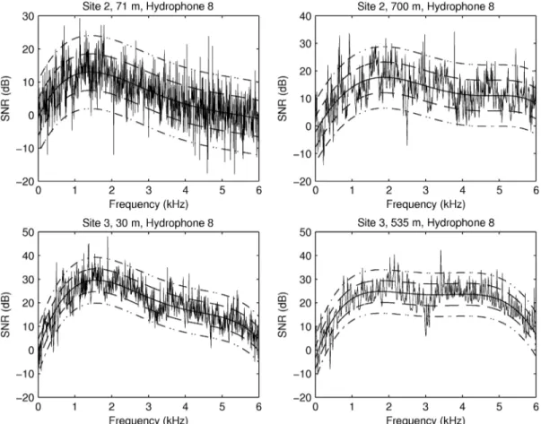
Fig. 5. SNR of cross-spectra between hydrophone 1 and hydrophone 8 for Site 2 (upper row) and Site 3 (lower row), at short (left column), and long range (right column). The smooth solid curve represents ; the dashed curves are ); the dotted-dashed curves are ).
allowing a potentially frequency-dependent (dispersive) sound speed for the path to be computed from measurements of the phase of the cross-spectrum. For a single nondispersive path with positive SNR in the received signal, will be a linear function of frequency. For multiple nondispersive paths, the phase function becomes more complicated, but is still distin-guishable from the random oscillations indicative of loss of SNR.
The preceding analysis is based on the correlation between source and receiver signals. In our case, the source signal is not available, but the received signals from multiple hydrophones in the vertical array are. Considering the source and receiver experimental arrangement of Fig. 1 as a single input/multiple output system, the cross-spectrum between the received signals at any two hydrophones is given by [12]
(4)
where represents the propagation path transfer function between the source and the th receiver. This can be rewritten in complex magnitude-phase form as
(5)
The physical interpretation of complex component of (5) is similar to that of (2). For a single nondispersive set of paths , , the phase of the cross-spectrum represents the path-delay difference between the source and each hydrophone. Deviations
in the measured cross-spectrum phase from a linear frequency dependence indicate contributions of multiple and/or dispersive paths to the signals received in each hydrophone.
B. Numerical Model
In order to test the validity of our approach, we have estab-lished a numerical model of the signals reflected by the seafloor. The acoustic field emitted by a point source and reflected by the seafloor is computed for each hydrophone at each frequency in the signal bandwidth [13]. This computation is based on a nu-merical evaluation of the Sommerfeld integral [14]
(6)
where is the grazing angle, is the sum of the source and the hydrophone heigths above the seafloor, is the distance between the source and the array, and is the plane wave reflection coefficient. This latter can be computed for a wide variety of structures [15], [16]: multilayer, fluid, solids, poro-elastic,
Then, the temporal signals for each hydrophone are obtained by an inverse Fourier transform
Fig. 6. Argument, wrapped phase, and unwrapped phase (from top to bottom) of cross-spectrum of signals received on hydrophones 1 and 2 for Site 2 at short distance (left) and for hydrophone 8 at Site 3 and at long range (right). The black curves correspond to the frequency part of the grey curves that satisfy (9).
The synthetic signals obtained are compared to experimental ones for Site 2 at long range on Fig. 4. The synthetic signals have a temporal structure very similar to the experimental sig-nals with three main peaks. A fourth peak, which can be be-cause of a deeper structure, can be seen on synthetic signals but not on experimental signals, maybe because of signal-to-noise ratio. Moreover, the time delay between each hydrophone is pre-cisely computed which is very important for phase studies.
IV. NOISE
A. SNR Definition
The SNR plays a key role in the data analysis. Indeed, in the case of low SNR, the phase of the cross-spectra has an erratic be-havior. Thus, it is necessary to define the SNR for our configura-tion and to compute it for each data set. But its definiconfigura-tion is com-plicated by two difficulties: 1) to the authors knowledge, there is no standard definition for the SNR of analysis of cross-spectra; and 2) we only have one realization of the signals for each con-figuration which precludes the use of averaging. Consequently, we have defined an ad-hoc SNR adapted to our problem.
For the study of cross-spectrum between hydrophone 1 and hydrophone , we first define the noise recorded by these trans-ducers by taking a part of the time recordings outside the
sig-nals. Then, we compute the autospectrum of reflected signals ( and ) and of noises ( and ). Fi-nally, the SNR is obtained with
SNR (8)
Practically, we use the SNR in decibels, i.e., SNR .
B. SNR Analysis
The SNR computation is presented in Fig. 5 for the four con-figurations (the two sites and the two distances) for the cross-spectrum between hydrophone 1 and hydrophone 8, located in the middle of the array. The results are similar for the other hy-drophones. To obtain these results, the signals were zero-padded to have the same number of points in the frequency domain for signals at long and short range, and to have enough points to correctly unwrap the phase. This zero-padding procedure is im-portant, particularly for short range measurements. Two com-ments can be made from these figures.
First, the evolution of SNR with frequency is erratic. This is mainly because of the fact that each analysis (for a given site, a given distance, and a given hydrophone) is based on a single realization without averaging. To smooth these curves, we have
Fig. 7. Phases of cross-spectra for Site 2 for hydrophones 2 to 6 (top), 7 to 11 (middle), and 12 to 15 (bottom) at short (left) and long (right) range. The solid curves are experimental data and dashed curves are synthetic data.
fitted them with a 5-order polynomial (written in the fol-lowing) and then we computed the RMS between the real curve and this fit . In Fig. 5, the curves , , and are plotted over the experimental curves. These curves allow us to define an heuristic confidence interval for our data.
Second, there are some peaks that lie above or below the con-fidence interval for some frequencies. More precisely, there is a
lowering of SNR around 3 kHz. This corresponds to the dip in the amplitude of the source spectrum (Fig. 3).
C. Definition of a Frequency Mask
The analysis of the phase of the cross-spectra being sensitive to the noise, we must define a threshold to accept or reject the signal. We have fixed this threshold at 6 dB which is a stan-dard value for this type of analysis. But a strict threshold that
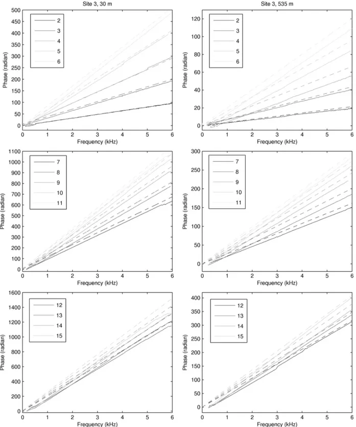
Fig. 8. Phases of cross-spectra for Site 3 for hydrophones 2 to 6 (top), 7 to 11 (middle), and 12 to 15 (bottom) at short (left) and long (right) range. The solid curves are experimental data and dashed curves are synthetic data.
rejects all the points with SNR below the threshold value is not appropriate for the erratic nature of the data. Consequently, we have adapted the threshold to our problem. We will only keep the points that verify the following condition:
AND AND
(9)
From this definition of the threshold, we build a frequency mask which allows us to keep or reject the points.
D. Noise Effects on Cross-Spectra
Fig. 6 (left) presents argument and phase (wrapped and un-wrapped) of cross-spectrum of signals received on hydrophones
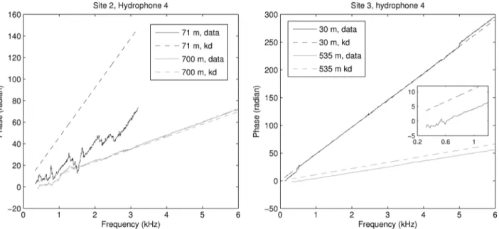
Fig. 9. Phases of cross-spectra for hydrophone 4 versus hydrophone 1 at short (black) and long (gray) range for Site 2 (left), and Site 3 (right). The solid curves are the experimental data and the dashed one are the lines. The inset shows a zoom on low-frequency for phases at long range for Site 3.
1 and 2 at Site 2 and short range. The same data are presented on Fig. 6 (right) for hydrophone 8 at Site 2 and long range.
These figures show that the noise has a strong influence on argument and phase of the cross-spectra and that this influence varies with the sites and the distances. Two effects are particu-larly shown: 1) a local low SNR; and 2) a low SNR on a larger frequency band.
The first effect (local low SNR) yields a jump in the un-wrapped phase. This effect is shown, for example, for Site 3 at long range (Fig. 6 right, bottom): the phase is linear with fre-quency, then an erratic behavior around 3 kHZ, and then is again linear with frequency. This effect is suppressed when the phase is computed only on masked data, i.e., for frequencies where data satisfy (9).
The second effect (low SNR on a larger frequency band) leads to a random frequency dependence of the phase and thus, im-possible to use. This effect is illustrated on Fig. 6 (left) which presents the results for Site 2 at short range for hydrophone 2. Above 3 kHz, the SNR is too low to give a correct estimation of the phase. On this example, we can also note two phases jump around 600 Hz and 1 kHz. Finally, the absence of points with sufficient SNR at low frequency leads to a shift of the phase. Consequently, the analysis should be based on relative phases and not on absolute phases.
V. COMPARISON OFMEASUREMENTS ANDSIMULATIONS
A. General Observations
The comparisons between phases of cross-spectrum obtained from experimental data and synthetic data are presented on Figs. 7 and 8 for the two sites and the two distances. In each of these four cases, we only computed the cross-spectra of hydrophone 1 versus hydrophone . Note that the phases scale is different from one figure to another. Note also that the data for Site 2 at 71 m go only up to 3.5 kHz when the other data
sets all extend to 6 kHz. This is because of the poor SNR for this configuration above 3.5 kHz (Fig. 6 left).
From these comparisons, three general comments can be made:
• accepting some residual problems because of noise, the comparisons are reasonable;
• for the two sites, the phase becomes linear with frequency at long range;
• the frequency behavior of phase is more complex for Site 2 than for Site 3, which is consistent with the geoacoustic structure of these two sites.
B. Detailed Analysis
1) Comparisons: When there is a single path regime
between one source and multiple receivers in a nondisper-sive medium, the phase of the cross-spectrum is linear with frequency (3): , being the separation between hydrophones and . This linear behavior is clearly seen on the previous figures and is shown with more details in Fig. 9 where the phases of the cross-spectra of hydrophone 4 versus hydrophone 1 are plotted for Sites 2 and 3 at short and long range. For Site 2, the phase is far from the curve at short range but becomes very close to it at long range for frequen-cies higher than 1500 Hz. For Site 3, the phase is very close to the curve at both short and long range, even for low frequency at short range. These Site 3 curves show also two interesting features that will have some consequences for the interpretation of other data. First, one can observe a small bump on the short range data around 5 kHz. This might be a noise effect as explained before. This indicates that, even though we eliminate the major part of the noise effects, there are still some residual problems that can lead to misunderstanding and, consequently, interpretation of data must be conducted with care. Second, because of noise effects at low frequency, some points are missing on experimental data and this can lead to a shift difference between experimental and synthetic curves and
TABLE III
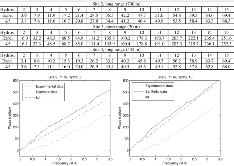
EXPERIMENTAL ANDTHEORETICALCROSS-SPECTRAPHASESLOPES(INrad/kHz)
Fig. 10. Phases of experimental and synthetic cross-spectra for hydrophone 8 (left) and 10 (right) versus hydrophone 1 at short range for Site 2.
even between two different experimental curves. Consequently, further comparisons between experimental and synthetic data will be with “linearized” data, where the linear behavior of the phase has been removed from the data.
In Table III, the slopes of the experimental curves (computed on their larger linear part) are compared to the corresponding values of for Site 2 at long range and Site 3 at short and long range. For these three cases, the experimental slopes and the values are close, the mean and the rms of the difference being always less than 1 rad/kHz.
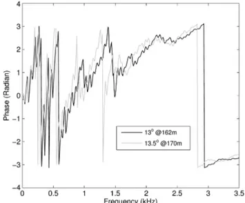
2) Some Particular Data: From Fig. 9 Site 3 long range/low
angle, it appears that the phase is linear at long range/low angles above about 600 Hz (see inset in Fig. 9). Thus, below 600 Hz, at low angles for Site 3, the cross-spectral phase is not linear indicating that a half-space approximation would not be partic-ularly good and also that the linear phase approximation would fail. Above 600 Hz, at low angles for Site 3 the phase is linear and layering may or may not be important. Given that we know that the sediment at the interface is granular and exhibits a crit-ical angle, it seems reasonable that above 600 Hz, the half-space assumption is acceptable.
In Fig. 10, the phases of cross-spectra for hydrophones 8 and 10 at short range for Site 2 are displayed. The phases are globally
increasing with frequency and their general behavior is close to the line. In this case, the matching between experimental and synthetic data is not very good. In particular, the experimental curves look convex while the synthetic curves look concave. This opposite behavior is particularly evident in the low fre-quency regime. For frequencies higher than 1.5 kHz, the shape of the phases become similar, in particular with bumps around 2400 Hz and 2800 Hz. But, even for these higher frequencies, there are differences between experimental and synthetic curves for one particular hydrophone, and moreover, these differences are not the same for another hydrophone even if this latter is close to the previous one (see the differences between the two plots on Fig. 10 for example). These differences that make these curves difficult to explain might be because of the high com-plexity of the seafloor on Site 2: the presence of numerous layers with some of them very thin lead to numerous acoustic paths which can be instable relative to the source-receiver angles and distance.
This complexity characteristic of Site 2 for short range data becomes simplified for long range data. The linearized phases (i.e., the real phase minus ) of hydrophone 3 for Site 2 at long range are plotted on Fig. 11 (left). The overall behavior of the experimental and synthetic data are similar, showing a distinct
Fig. 11. Linearized phases of cross-spectra for hydrophone 3 versus hydrophone 1 at long range for Site 2 (left) and for three different geoacoustic configurations of this Site (right): original is the “true” configuration, Mod. 1 and Mod. 2 are modifications described in the text.
change in character at 1500 Hz. Above 1500 Hz, the phase is very nearly linear. The small fluctuations in the measurements are due in part to multipath interference in the sediment layers. The salient point though is that the phase is clearly dominated by , i.e., a single path.
By contrast, for frequencies below 1500 Hz, the linearized phase show several distinct phase shifts. The experimental data show 3 phase shifts (one negative around 400 Hz and two positives around 800 Hz and 1200 Hz) whereas the synthetic data show two phase jumps (one negative around 800 Hz and one positive 1200 Hz). These phase jumps could be because of resonances inside the sediment stack. The resonances are caused by multipath interference within a layer at the condi-tion where , where is the vertical component of the wave number in the layer. If this were the correct explanation, the phase shifts should be ob-served in the spherical reflection coefficient. Fig. 12 does indeed show some phase shifts, however, they are not located at the same frequencies as in the experimental data. These discrepan-cies may be an indicator of small differences between the ground truth and the inverted geoacoustic model of the seafloor used for computing the synthetic data. In order to specifically iden-tify which layer(s) were responsible for the resonance effects, we computed the linearized phase for Site 2: keeping the global sound speed and density profiles but removing particular layers. The first modification (Mod. 1) removed the first layer where the sound speed is lower than the sound speed in the water and the second modification made (Mod. 2) is to remove the first layer and the second one where the sound speed is higher than in the layers below. The effects of these modifications are displayed on Fig. 11 (right). The obtained linearized phase for Mod. 1 con-figuration is nearly identical to the original except for an overall difference because of a jump at very low frequency. This re-sult indicates that this first layer is not very important for phase shifts at these angles. The obtained linearized phase for Mod. 2 is much different. In particular, the positive phase jump around 1200 Hz has disappeared. This indicates that this “fast” layer contributes to the 1200 Hz resonance for this geometry.
Fig. 12. Phase of the spherical reflection coefficient computed for Site 2 for positions of hydrophones 1 and 3.
VI. SUMMARY
In this paper, we have presented a detailed analysis of the phase of cross-spectra of signals reflected by two different seafloors (Site 2 is multilayered with acoustic basement at 150 m and Site 3 is composed of two layers above a basement at 15 m) and recorded on a vertical array. To the authors’ knowledge, this quantity is rarely used in underwater acoustics studies whereas we have shown that it contains useful information about the seafloor structure. One important point in this analysis is the influence of noise. Due to the experimental configuration used, we only have a single realization of the signal. Thus, we defined an empirical SNR that allows us to analyse our data with a frequency mask that rejects the points with a low SNR. Indeed, low SNR leads to random phases that can lead to misinterpretations. Moreover, missing points in the frequency band lead to a shift of the phase curve. Consequently, the analysis was conducted on relative and not absolute phases. All
these considerations concerning noise effects being taken into account, the comparisons between experimental and synthetic data are satisfactory. Two main points emerge from these comparisons. First, the subbottom plays an important role. This is shown in the low angle/long range data for Site 2 (below 1500 Hz) and Site 3 (below 600 Hz). At those frequencies a half-space approximation would be inappropriate. And second, at those frequencies, the linear reflection phase approximation would be violated.
The association of phase jumps in the cross-spectrum with layer resonances shown for Site 2 at long range opens the door for future work on the use of this technique to characterize fine-scale sediment structure in geoacoustic inversion methods.
ACKNOWLEDGMENT
The authors would like to thank the North Atlantic Treaty Or-ganization Underwater Research Center, La Spezia, Italy, under whose auspices the data were collected. They would also like to thank the Associate Editor, R. Chapman, and the two anony-mous reviewers whose comments have improved the paper.
REFERENCES
[1] D. Weston, “A moiré fringe analog of sound propagation in shallow water,” J. Acous. Soc. Amer., vol. 31, no. 6, pp. 617–654, 1959. [2] Z. Zhang and C. Tindle, “Complex effective depth of the ocean
bottom,” J. Acous. Soc. Amer., vol. 93, no. 1, pp. 205–213, 1993. [3] P. Joseph, “Complex reflection phase gradient as an inversion
param-eter for the prediction of shallow water propagation and the charac-terization of sea-bottoms,” J. Acous. Soc. Amer., vol. 113, no. 2, pp. 758–768, 2003.
[4] C. Holland and J. Osler, “High resolution geoacoustic inversion in shallow water: A joint time and frequency domain technique,” J. Acoust. Soc. Amer., vol. 107, pp. 1263–1279, 2000.
[5] C. Holland, R. Hollett, and L. Troiano, “A measurement technique for bottom scattering in shallow water,” J. Acoust. Soc. Amer., vol. 108, pp. 997–1011, 2000.
[6] S. Pinson and L. Guillon, “Sound speed profile characterization by the image source method,” J. Acous. Soc. Amer., vol. 128, no. 4, pp. 1685–1693, 2010.
[7] L. Guillon and C. Holland, “Cohérence de signaux réfléchis par le sol marin: modèle numérique et données expérimentales,” Traitement du signal, vol. 25, pp. 131–138, 2008.
[8] J. Berkson, “Measurements of coherence of sound reflected from ocean sediments,” J. Acoust. Soc. Amer., vol. 68, pp. 1436–1441, 1980. [9] P. Dahl, “Forward scattering from the sea surface and the van
cittert-zernike theorem,” J. Acous. Soc. Amer., vol. 115, pp. 589–599, 2004. [10] M. Siderius, P. Nielsen, and P. Gerstoft, “Range-dependent seabed
characterization by inversion of acoustic data from a towed receiver array,” J. Acous. Soc. Amer., vol. 112, no. 4, pp. 1523–1535, 2002. [11] S. Pinson, L. Guillon, and C. Holland, “Geoacoustic characterization
with an horizontal array by the image source method,” in Proc. 10th Eur. Conf. Underwater Acous., T. Akal, Ed., Istanbul, Turkey, Jul. 2010, pp. 229–237.
[12] J. Bendat and A. Piersol, Engineering Applications of Correlation and Spectral Analysis. New York: Wiley, 1980, ch. 3.
[13] J. Camin and C. Holland, On Numerical Computation of the Reflected Field From a Point Source Above a Boundary. 2006, personal commu-nication.
[14] L. Brekhovskikh and O. Godin, Acoustics of Layered Media. II: Point Sources and Bounded Beams. Berlin, Germany: Springer-Verlag, 1999, ch. 1.
[15] J.-F. Allard and N. Atalla, Propagation of Sound in Porous Media. Modelling Sound Absorbing Materials. New York: Wiley, 2009, ch. 7.
[16] P. Cervenka and P. Challande, “A new efficient algorithm to compute the exact reflection and transmission factors for plane waves in layered absorbing media (liquids and solids),” J. Acous. Soc. Amer., vol. 89, pp. 1579–1589, 1991.
Laurent Guillon received the B.Sc. degree in
physics from the University of Nantes, France, in 1994. He received the M.Sc. and Ph.D. degrees in acoustics from the University of Le Mans, France, in 1995 and 1999, respectively.
From 1999 to 2001, he worked as a Postdoctoral student in the Laboratory for Mechanics and Acous-tics (CNRS-LMA) in Marseille, France. Since 2001, he has been an Associate Professor at the French Naval Academy, Brest, France. In 2006, he spent six months in the Applied Research Laboratory at Penn State University, State College, as a visiting professor. His research interests include sediment acoutics, scattering modeling, seafloor characterization, and low-frequency acoustic penetration in seafloor.
Dr. Guillon is a member of the Acoustical Society of America and of the French Society of Acoustics.
Charles W. Holland received the B.Sc. degree in
engineering from the University of Hartford, Hart-ford, CT, in 1983, and the M.Sc. and Ph.D. degrees in acoustics from the Pennsylvania State University, State College, in 1985 and 1991, respectively. His Ph.D. thesis addressed acoustic propagation through poro-viscoelastic marine sediments.
In 1985, at Planning Systems Inc., Virginia, he conducted research on geoacoustic modeling, seafloor classification techniques, high frequency seafloor acoustic penetration, and low to midfre-quency bottom loss/bottom scattering measurement and modeling techniques. He joined the research staff at the NATO Undersea Research Centre, La Spezia, Italy, in 1996, where he developed seabed reflection and scattering measure-ment techniques in support of propagation and reverberation prediction. In 2001, he joined the Applied Research Laboratory at the Pennsylvania State University where he continues his research in many aspects of seabed acoustics.
Dr. Holland is a fellow of the Acoustical Society of America.
Christopher Barber (M’11) received the B.Sc.
de-gree in engineering physics from the University of Tennessee in 1990, and the M. Eng. and Ph.D. de-grees in acoustics from the Pennsylvania State Uni-versity, State College, in 1996 and 2004, respectively. In 1991, he joined the Naval Surface Warfare Center, Carderock Division, where he worked for 13 years in the areas of ship acoustic test and evaluation, sonar self-noise, susceptibility analysis, and ship silencing research and development. His experience at NSWC includes at-sea acoustic tests of combat ships, submarines and research vessels, as well as water tunnel and large scale model acoustic testing. He joined the Applied Research Laboratory at Penn State in 2004, and is currently engaged in research related to short range/near field acoustic propagation, development of ship radiated noise models, and modeling of propulsor and flow-related sonar self-noise.He teaches courses in Audio Engineering and Electrical Engineering at Penn State.
Dr. Barber is a member of the Acoustical Society of America and the Audio Engineering Society.