HAL Id: hal-01140310
https://hal-mines-paristech.archives-ouvertes.fr/hal-01140310
Submitted on 8 Apr 2015
HAL is a multi-disciplinary open access
archive for the deposit and dissemination of sci-entific research documents, whether they are pub-lished or not. The documents may come from teaching and research institutions in France or abroad, or from public or private research centers.
L’archive ouverte pluridisciplinaire HAL, est destinée au dépôt et à la diffusion de documents scientifiques de niveau recherche, publiés ou non, émanant des établissements d’enseignement et de recherche français ou étrangers, des laboratoires publics ou privés.
Romain Lerallut, Etienne Decencière, Fernand Meyer
To cite this version:
Romain Lerallut, Etienne Decencière, Fernand Meyer. Image Filtering Using Morphological Amoebas. 7th international symposium on mathematical morphology, 2005, Paris, France. �10.1007/1-4020-3443-1_2�. �hal-01140310�
IMAGE FILTERING USING MORPHOLOGICAL AMOEBAS
Romain Lerallut, Étienne Decencière, Fernand Meyer
Centre de Morphologie Mathématique, École des Mines de Paris 35 rue Saint-Honoré, 77305 Fontainebleau, France
Abstract This article presents the use of anisotropic dynamic structuring elements, or amoebas, in order to build content-aware noise reduction filters. The amoeba is the ball defined by a special geodesic distance computed for each pixel, and can be used as a kernel for many kinds of filters and morphological operators.
Keywords: Anisotropic filters, noise reduction, morphological filters, color filters
1.
Introduction
Noise is possibly the most annoying problem in the field of image process-ing. There are two ways to work around it: either design particularly robust algorithms that can work in noisy environments, or try to eliminate the noise in a first step while losing as little relevant information as possible and conse-quently use a normally robust algorithm.
There are of course many algorithms that aim at reducing the amount of noise in images. In mathematical morphology filters can be, broadly-speaking, divided into two groups:
1 alternate sequential filters based on morphological openings and clos-ings, that are quite effective but also remove thin elements such as canals or peninsulas. Even worse, they can displace the contours and thus cre-ate additional problems in a segmentation application.
2 reconstruction filters, such as levelings, that reconstruct faithfully the contours, sometimes in a too faithful way when the contour itself is cor-rupted by noise. This can cause great problems in some applications, such as 3D visualization, which rely heavily on clean contour surfaces.
They are often combined, but it can be difficult to control what will be erased and what will be reconstructed, so a new approach was proposed.
2.
Amoebas: dynamic structuring elements
Principle
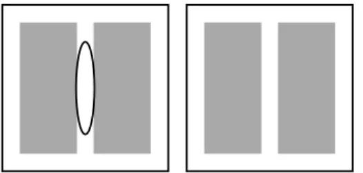
Classic filter kernel. Formally at least, classic filters work on a fixed-size sliding window, be they morphological operators (erosion, dilation) or convo-lution filters, such as the diffusion by a gaussian. If the shape of that window does not adapt itself to the content of the image (see figure 1), the results de-teriorate. For instance, an isotropic gaussian diffusion smooths the contours when its kernel steps over a strong gradient area.
Figure 1 Closing of an
im-age by a large structuring ele-ment. The structuring element does not adapt its shape and merges two distinct objects.
Amoeba filter kernel. Having made this observation, Perona and Malik [1] (and others after them) have developed anisotropic filters that inhibit diffu-sion through strong gradients. We were inspired by these examples to define morphological filters whose kernels adapt to the content of the image in order to keep a certain homogeneousness inside each structuring element (see fig-ure 2). The interest of this approach, compared to the analytical one pioneered by Perona and Malik is that it does not depart greatly from what we use in mathematical morphology, and therefore most of our algorithms can be made to use amoebas with little additional work. Most of the underlying theoretical groundwork has been described by Jean Serra in his study [3] of structuring functions, although until now it has seen little practical use.
Figure 2 Closing of an
im-age by an amoeba. The amoeba does not cross the contour and as such preserves even the small canals.
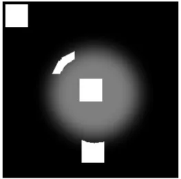
The shape of the amoeba must be computed for each pixel around which it is centered. Figure 3 shows the shape of an amoeba depending on the posi-tion of its center. Note that in flat areas such as the center of the disc, or the
Amoebas: dynamic structuring elements 3
Figure 3 Shape of an amoeba at various positions on an image.
background, the amoeba is maximally stretched, while it is reluctant to cross contour lines.
When an amoeba has been defined, most morphological operators and many other types of filters can be used on it: median, mean, rank filters, erosion, di-lation, opening, closing, even more complex algorithms such as reconstruction filters, levelings, floodings, etc.
Construction
Amoeba distance. In general, a filtering kernel of radiusr is formally
de-fined on a square (or a hexagon) of that radius, that is to say on the ball of radiusr relative to the norm associated to the chosen connectivity. We will
keep this definition changing only the norm, using one that takes into account the gradient of the image.
Definition. Letdpixel be a distance defined on the values of the image, for
example a difference of gray-value, or a color distance.
Letσ = (x = x0, x1, . . . , xn= y) a path between points x and y. Let λ be
a real positive number. The length of the pathσ is defined as L(σ) =
n
X
i=0
1 + λ.dpixel(xi, xi+1)
The “amoeba distance” with parameterλ is thus defined as: ½
dλ(x, x) = 0
dλ(x, y) = minσL(σ)
It it important to realize thatdpixelhas no geometrical aspect, it is a distance
the number of pixels of a pathσ, then L(σ) ≥ n (since λ ≥ 0), which bounds
the maximal extension of the amoeba.
This distance also offers an interesting inclusion property:
Property. At a radiusr given the family of the balls Bλ,r relative to the
dis-tancedλis decreasing (for the inclusion),
0 ≤ λ1 ≤ λ2 ⇒ ∀(x, y), dλ1(x, y) ≤ dλ2(x, y) ⇒ ∀r ∈ R+, B
λ1,r ⊃ Bλ2,r
Which may be useful when building hierarchies of filters, such as a family of alternate sequential filters with strong gradient-preserving properties.
The pilot image. We have found that because of the noise it is better not to use directly the original image to compute the shape, but first to use a strong smoothing filter. However, it is crucial that this filter only dampen the noise while preserving as much as possible the larger contours.
A large gaussian works fairly well, and can be applied very quickly with advanced algorithms, however we will see below that iterating amoeba filters yields even better results.
3.
Amoebas in practice
Adjunction
Erosions and dilations can easily be defined on amoebas. However it is nec-essary to use adjoint erosions and dilations when using them to define openings and closings:
δ(X) = S
x∈XBλ,r(x)
²(X) = {x/Bλ,r(x) ⊂ X}
These two operations are at the same time adjoint and relatively easy to compute, contrary to those that use the transposition.
Algorithms
The algorithms used for the erosion and dilation are quite similar to those used with regular structuring elements, with the exception of the step of com-puting the shape of the amoeba:
Erosion (grey-level): for each pixelx:
compute the shape of the amoeba centered onx
compute the minimumM of the pixels in the amoeba
Results 5
Dilation (grey-level):
for each pixelx:
compute the shape of the amoeba centered onx
for each pixely of the amoeba:
value(y)=max(value(y),value(x))
The opening that uses those algorithms can be seen as the grey-level exten-sion of the classic binary algorithm of taking the set of all the centers of the circles that fit inside the shape (erosion), and then returning the union of all those circles (dilation).
Complexity
The theoretical complexity of an simple amoeba-based filter (erosion, dila-tion, mean, median) can be approximated by:
T (n, k, op) = Ohn ∗³op(kd) + amoeba(k, d)´i
Wheren is the number of pixels in the image, d is the dimensionality of the
image (usually 2 or 3),k is the maximum radius of the amoeba, op(kd) is the
cost of the operation andamoeba(k, d) is the cost of computing the shape of
the amoeba for a given pixel.
The shape of the amoebas is computed by a common region-growing imple-mentation using a priority queue. Depending on the priority queue used, the complexity of this operation is in slightly more thanO(kd) (see [4] and [5] for
advanced queueing data structures).
Therefore, for erosion, dilation or mean as operators, we have a complex-ity of a little more than O(n ∗ kd) which is the complexity of a filter on a
fixed-shape kernel. It has indeed been verified in practice that, while being quite slower than with fixed-shape kernels, filters using amoebas tend to fol-low rather well the predicted complexity, and do not explode.
4.
Results
Alternate sequential filters
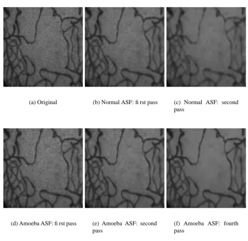
The images of figure 4 compare the differences between alternate sequential filters built on classic fixed shape kernels and ASFs on amoebas in the filtering of the image of a retina. The filter should be able to reduce the amount of background noise while preserving the vessels.
Median and mean
In the context of image enhancement, we have found that a simple mean or median coupled with an amoeba forms a very powerful noise-reduction filter.
(a) Original (b) Normal ASF: first pass (c) Normal ASF: second pass
(d) Amoeba ASF: first pass (e) Amoeba ASF: second pass
(f) Amoeba ASF: fourth pass
Figure 4. Alternate sequential filters on classic kernels and on amoebas. The amoeba preserve extremely well the blood vessels while strongly flattening the other areas.
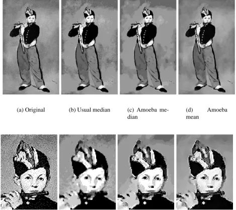
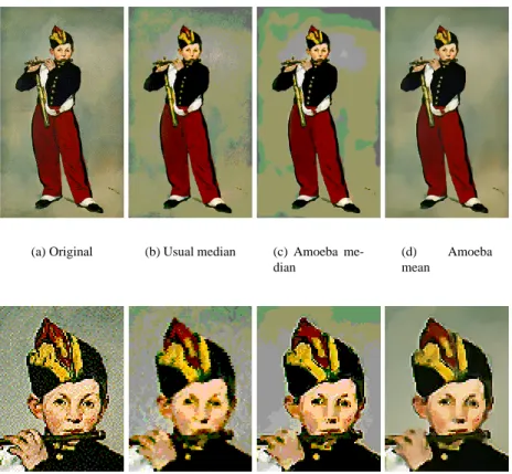
The images in figure 5 show median and the mean computed on amoebas compared to those built on regular square kernels. The pilot image that drives the shape of the amoeba is the result of a standard gaussian filter of size 3 on the original image, and the distancedpixelis the absolute difference of grey-levels.
For the filters using amoebas, the median filter preserves well the contour, but the mean filter gives a more “aesthetically pleasing” image. In either case, the results are clearly superior to filterings by fixed-shape kernels, as seen in the figure 5.
Mean and median for color images
In the case of color images, the mean is replaced by the mean on each color component of the RGB color space. For the “median”, the point closest to the barycenter is chosen.
Results 7
(a) Original (b) Usual median (c) Amoeba me-dian
(d) Amoeba
mean
Figure 5. Results of a “classic” median filtering and two amoeba-based filterings: a median and a mean on Edouard Manet’s painting “Le fifre”.
The choice of the color space and the distance has an impact on the quality of the result. However the most noticeable impact is that of the choice of the pilot image. For the images in figure 6, we have used a gaussian filter of size 3 on each R,G and B component, and recombined the three channels.
Iteration
The quality of the filtering strongly depends on the image that determines the shape of the amoeba. The previous examples have used the original image filtered by a gaussian, but this does not always yield good results.
It is frequent indeed that a small detail of the image be excessively smoothed in the pilot image, and thus disappears completely in the result image. On the other hand, noisy pixels may be left untouched if the pilot image does not eliminate them. A possible solution is to somewhat iterate the process, using
(a) Original (b) Usual median (c) Amoeba me-dian
(d) Amoeba
mean
Figure 6. Color images: results of a “classic” median filtering, and two amoeba-based filter-ings: a median and a mean.
the first output image not as an input for filtering, as it would commonly be done, but as a new pilot image instead.
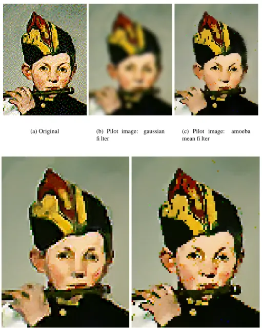
In practice, for noise-reduction purposes, only two iterations are needed. The first one follows the scheme described earlier, using the gaussian-filtered original image as a pilot, with aggressive parameters, and outputs a well-smoothed image in flat areas while preserving as much as possible the most important contours. The second iteration takes the original image as input and the filtered image as a pilot, with less destructive parameters, and preserves even more the finer details, while removing a lot of the noise.
Figure 7 shows the two steps of the process. Note in particular how the fifer player’s left hand is preserved with the iterated amoebas, while it is strongly degraded with the gaussian-filtered pilot image.
Conclusion and future work 9
(a) Original (b) Pilot image: gaussian filter
(c) Pilot image: amoeba mean filter
(d) Result image: amoeba mean with gaussian pilot
(e) Result image: amoeba mean with amoeba pilot
Figure 7. Using an amoeba-based mean filter can create a roughly smoothed image that does not create an excessive blur and can thus be used as a better pilot image for further filtering. Note the difference on the hand and the eyebrows. With the amoeba-piloted filter, the hand is well preserved, and the eyebrows do not begin to merge with the eyes, as is the case in the gaussian-piloted filter.
5.
Conclusion and future work
We have presented here a new type of structuring element that can be used in many morphological algorithms. By taking advantage of outside informa-tion, filters built upon those structuring elements can be made more robust on noisy images and in general behave in a “more sensible” way than those based on fixed-shape structuring elements. In addition, morphological amoebas are very adaptable and can be used on color images as well as monospectral ones and, like most morphological tools, they can be used on images of any dimen-sion (2D, 3D, . . . ). Depending on the application, two categories of filters are available. On the one hand, alternate sequential filters are very effective when looking for very flat zones, whereas median and mean filters output smoother images that may be more pleasing to the eye but could be harder to segment.
It is possible to use amoebas to create reconstruction filters and floodings that take advantage of the ability to parameterize the shape of the amoebas based on the image content. However, the behaviors of the amoebas are a lot more difficult to take into account when they are used in such complex al-gorithms. In particular, amoebas often have a radius larger than one, so for instance the identification made between conditional dilation and geodesic di-lation is no longer valid.
As usual when adapting a technique developed for grey-level images to color images, a lot of application-dependent empirical work must be done to select which color spaces and which distances provide the “best” results. The results show that simple extensions of the scalar algorithms to the RGB space already yield excellent results, especially when iterating. The use of more “perceptual” distances (HLS or LAB) would probably prevent most unwanted blending of features, although this is as yet conjectural and will be the basis of further work.
References
[1] Perona, P. and Malik, J., “Scale-space and edge detection using anisotropic diffusion”,
IEEE Transactions on Pattern Analysis and Machine Intelligence, vol. 12, no. 7, July 1990
[2] Wei, G. W., “Generalized Perona-Malik equation for image restoration”, IEEE Signal
Pro-cessing Letters, vol. 6, no. 7, July 1999
[3] Serra, J. et al, “Mathematical morphology for boolean lattices”, Image analysis and
math-ematical morphology - Volume 2: Theoretical advances, Chapter 2, pp 37-46, Academic
Press, 1988
[4] Cherkassky, B. V. and Goldberg, A V., “Heap-on-top priority queues”, TR 96-042, NEC Research Institute, Princeton, NJ, 1996
[5] Brodnik, A. et al., “Worst case constant time priority queue”, Symposium on Discrete Algorithms, 2001, pp 523-528