An analytical model with interaction between species for growth and dissolution of precipitates

HAL Id: hal-01552398

https://hal-mines-paristech.archives-ouvertes.fr/hal-01552398

Submitted on 2 Jul 2017

HAL is a multi-disciplinary open access

archive for the deposit and dissemination of sci-entific research documents, whether they are pub-lished or not. The documents may come from teaching and research institutions in France or abroad, or from public or private research centers.

L’archive ouverte pluridisciplinaire HAL, est destinée au dépôt et à la diffusion de documents scientifiques de niveau recherche, publiés ou non, émanant des établissements d’enseignement et de recherche français ou étrangers, des laboratoires publics ou privés.

An analytical model with interaction between species for

growth and dissolution of precipitates

Gildas Guillemot, Charles-André Gandin

To cite this version:

Gildas Guillemot, Charles-André Gandin. An analytical model with interaction between species for growth and dissolution of precipitates. Acta Materialia, Elsevier, 2017, 134, pp.375 - 393. �10.1016/j.actamat.2017.04.035�. �hal-01552398�

1

An analytical model with interaction between species

for growth and dissolution of precipitates

Gildas GUILLEMOT, Charles-André GANDIN MINES ParisTech, PSL Research University,

CEMEF UMR CNRS 7635

CS10207, 06904 Sophia Antipolis, France

Abstract

An analytical model for growth in a semi-infinite matrix with cross-diffusion between species is presented. Application is given for precipitation of the -phase in the -matrix during isothermal holding at 600 °C in the Ni – 7.56 at.% Al – 8.56 at.% Cr alloy. The exact time-dependent solutions for the solute profiles and the growth kinetics are validated with a numerical front-tracking simulation. The simulation of cross diffusion terms in a multicomponent alloy is thus demonstrated. Extension of the analytical solution is given for growth in a matrix of finite size. The driving force is then based on a mathematical estimation of the far-field composition. The Gibbs-Thomson effect is also accounted for to consider the effect of curvature on the equilibrium tie-lines. Comparison of analytical solution with the numerical front-tracking simulation shows excellent agreement. Results also point out the detrimental approximation of using the average composition of the matrix for computing the driving force as well as the limitation of the solution proposed by Chen et al. [Acta Mater. 56 (2008) 1890]. A detailed discussion is finally given on the origin of oscillations observed for the time evolution of the precipitate radius which alternates between growth and dissolution regimes, pointing out the combined role of solute fluxes and tie-lines compositions at the precipitate/matrix interface.

Keywords

2

1. Introduction

Industries make significant use of precipitation processing to enhance in-service mechanical properties of metallic alloys. The precipitation process is triggered by heat treatments and leads to the development of fine particles of a novel phase – often referred to as precipitates – dispersed in a pre-existing mother phase – hereafter referred to as matrix phase. One of the goals of precipitation processes is to form obstacles to the movement of dislocations and thus increase the yield strength of the material. The presence of precipitates may also affect grain boundary motion by means of the Zener pinning effect [1]. However, the control of the size distribution of the precipitates remains difficult as it is the consequence of complex processes where nucleation, growth and coarsening of the particles concomitantly take place. Nevertheless, coarsening can be seen as the result of mass exchanges taking place at interfaces between collections of particles embedded in the same matrix phase. It manifests itself as the consequence of growth and dissolution of a population of precipitates controlled by chemical diffusion of species. Consequently, nucleation and growth/dissolution are thus the basic mechanisms by which the precipitation kinetics is controlled. The metallurgist community very soon identified these two cornerstones for the tailoring of heat treatments in order to reach targeted microstructural features and hence end-use mechanical properties [2, 3, 4]. At first coupled with nucleation and coarsening models, analytical approximations for precipitate growth could provide with global precipitation kinetics [7, 8]. Numerical tracking of the particle size distribution (PSD) was then achieved [9, 10], providing the possibility to deal with non-isothermal heat treatments [11], multicomponent alloys [12, 13] or even coupling with long range diffusion processes [14, 15] for the prediction of particle free zones at grain boundary.

But recent simulations were also carried out with the goal to reach a direct representation of the precipitates in an elementary volume, for instance using the Monte-Carlo method [16]. Comparison of simulations with Atom Probe Tomography (APT) for chosen ternary alloys subject to interrupted isothermal holding clearly revealed the role of interaction between chemical species on the diffusion kinetics and the effect of curvature on thermodynamic equilibrium. These results justified recent efforts to introduce systematic coupling with thermodynamic and kinetics databases [13, 14, 15, 17, 18]. However, while global PSD precipitation models offer versatility for the design of heat treatments in industrial alloys [15], reliability of their approximate growth kinetics is not yet well established. Spreading and success of numerical tools developed to meet the growing industrial needs in metal forming processing [19] still requires efforts to improve and validate previously developed growth kinetics.

Few models are yet available that account for multicomponent growth kinetics [11, 17, 20, 21]. Du and Friis [22] recently demonstrated their limitations. Large differences were observed for various alloys and thermodynamic databases. These comparisons showed the need to revisit and validate an analytical solution for the grow kinetics of precipitates and to discuss usual hypotheses encountered in the literature.

3

The present contribution only focusses on growth/dissolution processes. An analytical model previously derived for solidification of globulitic grains in multicomponent alloys [23, 24] is extended and applied to precipitation. The mathematical model and its assumptions are first introduced. A numerical front-tracking method is then described, followed by the exact analytical solution of the mathematical model. A set of validations based on precipitation in a Ni-Al-Cr ternary alloy are proposed. Extensions of the analytical solution include the treatment of a non-stoichiometric precipitate and the role of curvature on the interfacial equilibrium, while the far-field composition that controls the driving force is estimated with integration of the solute profiles as previously proposed [23]. The present model requiring the treatment of dissolution, a generalized Laplace solution including cross diffusion is also introduced. Finally, an oscillation regime showing alternate growth and dissolution is identified as part of the evolution of the system toward its thermodynamic equilibrium. It is discussed in details in order to identify its origin and its possible consequences on the precipitation process.

2. Mathematical model

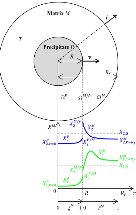
A single precipitate of phase growing in a matrix phase is schematized in Figure 1. Its geometry is assumed one-dimensional (1D), with radius and growth velocity only made of a unique component along the radial unit vector ̂. The matrix domain adopts the same spherical geometry. It is limited by radius defining the volume of the system . This volume may simply be set proportional to the inverse of the density of precipitates per unit volume. The domains defining the precipitate, , and the matrix, , are separated by a phase interface, , located at at a given time . The molar volume, , is assumed equal and constant in the and phases. A multicomponent alloy is considered with solute elements added to the solvent element. In Fig. 1, only the solute profiles in phases and of two elements – indexed 1 and 2 – are schematized. For solute species in phase , the molar compositions satisfy the mass conservation equations:

[∑ ( )] with { } and ( ) { } (1)

where the diffusion matrix is hereafter assumed homogeneous in each domain. The term in square brackets represents the diffusion flux associated to element in phase , . It is a summation over the -components located on the -line of the diffusion matrix, , multiplied by the corresponding solute gradient of element , with { }. The cross diffusion phenomena is induced by the non-diagonal terms in the diffusion matrix, thus contributing to a diffusion flux of element due to the local composition gradient of element in phase , ( ), with and { }. According to the solute balance at the interface, the precipitate growth velocity depends upon the interfacial compositions in the matrix, , and in the precipitate,

_{, as well as on the composition gradients at the interface in the matrix,}

, and in the precipitate, _:

4

( ⁄ ⁄ ) ∑ ( ⁄ _{) ∑ (}

⁄ )

with ( ) { } (2)

We assume no solute exchange at the external boundary of the system. This could be justified by considering symmetry of solute mass exchange at when several precipitates interact through the matrix. Similarly, the solute flux is null at the center of the precipitate domain, i.e. for These two conditions then write for all species :

∑

with ( ) { } (3a)

∑

with ( ) { } (3b)

No solute flux being present at its boundaries and no mass source being assumed in its volume, the average molar composition of the whole system is kept unchanged and equal to the nominal composition, ( ). Thermodynamic equilibrium is also assumed at the phase interface . The interfacial compositions are thus given by the tie-lines of the phase diagram computed at the system temperature and in the presence of the Gibbs-Thomson effect, i.e. accounting for the radius of curvature of the precipitates, . The set of interfacial compositions,

_and ⁄ _{, are given by the mathematical relations:}

⁄ ₍ ⁄ _{) (4a)}

⁄ ⁄ ₍ ⁄ _{) with { } (4b)}

where _{relates the temperature to the solvus surface of the phase diagram defined by the matrix}

composition _{and the radius , while gives the composition of the -component in the}

precipitate when knowing the equilibrium matrix composition _{and its radius .}

A very small nucleus is initially present. Its composition is uniform. The initial matrix composition, also uniform, is , thus neglecting the effect of the nucleus on the global mass balance of the system. As the model is thereafter presented and applied for a fixed and homogeneous temperature, , the nominal composition is chosen within the two-phase region of the phase diagram thus promoting precipitate growth. It should be pointed out that imposing the temperature does not correspond to an adiabatic condition. It was previously shown that coupling of precipitate growth with temperature evolution is possible considering a global energy balance [23].

3. Numerical model

A numerical solution of the set of Eqs 1-4 has been developed with a so-called front tracking approach. It is based on the Landau transform [25] already used by the authors [23, 26, 27]. Normalized coordinates, and , are respectively defined for the precipitate and matrix phases as and ( ) ( ), as schematized in Fig. 1, thus always maintaining the interface position at and . The conservation equations (Eq. 1) are rewritten for both the -phase and the -phase using and as the reference frame, respectively. Moreover, the solute flux balance at the -interface (Eq. 2) is rewritten for the fixed Landau coordinates and . Similarly, the conditions fixing the solute fluxes at the boundaries of the

5

system are rewritten at (Eq. 3a) and (Eq. 3b). A regular grid is initially defined for both phases. All equations are discretized in Landau’s coordinate system. They are solved at any time using an implicit time-stepping incremental procedure that covers the whole precipitation sequence. The solute balance equations (Eq. 2) for all species are considered with an estimation of the solute flux deduced from the current composition field and the tie-lines (Eqs 4). These latter equations are solved with a simplex method [28]. A detailed presentation of the numerical development is given elsewhere [23].

4. Analytical model

4.1. Exact solution

An analytical solution of Eqs (1)-(4) exists for a semi-infinite medium ( ) [23, 24]. It is an extension of the work originally presented by Zener [2] and Aaron et al. [4] for growth limited by diffusion of a unique solute specie in a binary alloy, also derived by Carslaw and Jaeger [29] for growth limited by diffusion of energy for a pure substance. Analytical expression for spherical geometries was also proposed by Horvay and Cahn [5]. Martin et al. [6] also reported the same laws with extension to various geometries. The analytical solution of Eqs (1)-(4) is seen as a generalization for cross diffusion of species in multicomponent alloys. The steps of the resolution may also be compared with the one proposed by Hunziker [30] for the stability analysis of a planar interface developed as part of a dendrite tip kinetics model. It should be pointed out that this approach makes use of a diagonalization procedure which is comparable with the developments by Vermolen et al. [31]. Considering a semi-infinite matrix phase at a fixed temperature and further neglecting the curvature effect, both interfacial solute compositions and are kept constant upon growth. Consequently the solute composition is uniform in the precipitate and given by the interfacial composition. In the matrix phase, the solute profiles are time and space dependent. For any component, it was demonstrated that the only possible analytical solution is given by:

( ) ∑ ( ) with { } (5)

where is the matrix composition at infinite distance from the interface, is the local radial position, is the current time, is the -eigenvalue of the diffusion matrix , with { },

is the -component of the -unitary eigenvector of matrix , , with ( ) { }. The

matrix defined with the components will be denoted hereafter as the eigenmatrix, . The set of

-values , with { }, are still to be determined. The function ( ) is written slightly differently compared to Aaron et al. [4], yet leading to the same values for given radius, , and time, :

( )

√

√ ₍√ ₎

(6) The coefficients are given by the matrix vector product:

6

where the vector corresponds to the difference between the interfacial matrix composition and the composition at infinity ( with { }) and the ( ) matrix is given by:

( )

(

)

with ( ) { } (8) where is the ( ) component of the inverse eigenmatrix, . The parameter1 is still an unknown coefficient defining the growth velocity of the spherical precipitate. It was demonstrated [23] that this key parameter is related to the precipitate radius by the simple relation:

(9)

providing that the growth is initiated at when . It should be pointed out that the relation (9) is still valid for any 1D geometry and can consequently be extended to cylindrical and planar geometry as detailed in Appendix A. The time derivation of Eq. 9 gives the growth velocity, , and hence the equivalent expression:

(10)

The parameter is computed as the solution of a second matrix system related to the solute balance at the interface (Eq. 2). Considering constant compositions at the interface both for the precipitate phase and for the matrix phase (i.e. no curvature effect, fixed temperature and semi-infinite matrix), the solute flux in the precipitate can be neglected so the system becomes [23]:

_{( ) (11)}

where the vector corresponds to the variation of interfacial composition between matrix and precipitate (with components , { }) and the components of the ( ) matrix are expressed as:

( ) ∑ ( ) with ( ) { } (12)

where the ( ) function is linked to the ( ) function by: ( ) _{( )}( )

( √ √ (√ )) (13)

The set of equations (Eqs 4 and 11) can be solved considering thermodynamic equilibrium at the interface. Diagonalization of the diffusion matrix is simply required to extract the eigenvalues and the unitary eigenvectors. The corresponding unknowns are the interfacial compositions, and , plus the parameter. When a linear approximation of the phase diagram is considered, the compositions at the interface are linked by fixed partition coefficients using the relationship with { }, thus defining simple functions (Eq. 4b). However, relations are usually non-linear for realistic phase diagram and should be solved

1_{The choice of the notation}

by the authors for the growth parameter is explained by the need to differentiate this value to the one, , used in the previous mathematical development [23]. However the two parameters are simply linked by the relation .

7

using an iterative approach. The simplex method is once more well suited for determining the solutions [28]. It is a vertices polyhedron and each vertex corresponds to interfacial compositions of the components of the matrix composition , as these compositions are linked by Eq. 4a for a fixed temperature, . After resolution, all interfacial compositions are known as well as the parameter which gives the growth kinetics. The radius, , and the velocity, , are then given for any time, , using Eq. 9. If required, the current composition profile, at the same time , is expressed with Eq. 5 where the vector is directly given by Eq. 7. The same approach of resolution can also be applied for the others 1D geometrical approximations considering the associated ( ) and ( ) functions (Appendix A).

4.2. Application

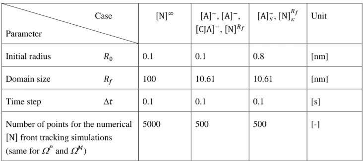
We first compare simulations with the analytical and numerical models for the growth of a precipitate in a semi-infinite matrix at a fixed temperature. The choice of the system is given in Table 1. It is inspired from one of the configuration studied by Booth-Morrison et al. [32] and Mao et al. [16] by APT, later also considered by Rougier et al. [13, 15]. The alloy composition is Ni - 7.56 at.% Al - 8.56 at.% Cr and the aging temperature is 600 °C. The corresponding isothermal section of the phase diagram is given in Figure 2. The precipitating phase – the -phase – is expected to grow at the expense of the matrix phase – the -phase –. The atomic structure of the -phase is disordered face-centered cubic while the -phase adopts the L12 ordering structure.

Thermodynamic equilibrium computations are performed with the NI20 thermodynamic database [33]. When phases are at equilibrium, the Cr-composition in the -phase is slightly lower than in the -phase. Contrarily, the Al-composition in the -phase is largely higher than in -phase as illustrated by the tie-lines in Fig. 2. It is worth mentioning the adoption of a tabulation strategy for Eqs (4), thus avoiding direct call to the thermodynamic equilibrium computation by storing the solvus surface and the tie-lines of the phase diagram. Also to be noticed is the small difference of the molar volumes between the -phase and the -phase at equilibrium, of the order of 1 % [33], thus justifying the similar molar volumes hypothesis introduced in the models.

In order to validate the exact solution proposed in section 4.1, the numerical front tracking simulation (section 3) is applied to the development of an isolated precipitate in a large spherical domain where boundary effects can be neglected. As curvature effect is not considered in this first validation, the phase diagram corresponds to the one computed without curvature in Fig. 2 (plain line – ). For in-depth validation, we hereafter consider four different diffusion matrices for the matrix -phase. Values of the matrices are given in Table 2. The full diffusion matrix, ,

was derived by Rougier et al. [13] and calculated from literature data [16]. This matrix is modified in by keeping the coefficient unchanged but forcing the coefficient to a nil value (similarly in by keeping the coefficient unchanged but forcing the coefficient to

a nil value). This operation permits removing the effect of Cr on the flux of Al for (or

removing the effect of Al on the flux of Cr for ). The last matrix, , is purely diagonal, i.e.

with non-diagonal coefficients forced to nil values, thus fully ignoring cross-diffusion phenomena. Comparison of simulations using the four diffusion matrices is also used to reveal the effect of the

8

cross diffusion terms on the growth kinetics of the precipitate. The diffusion matrix for the precipitate -phase is chosen diagonal with artificially large values to ensure homogeneous solute composition. The size of the simulation domain for the numerical model, , is large enough to mimic the growth in an infinite domain and achieve comparison with the exact analytical solution. The conditions for the various computations are presented in Tables 3 and 4. Figure 3 shows the time evolution for the radius and the velocity, together with the selected interface compositions read on the working tie-line, for the 4 diffusion matrices. In order to help comparisons and discussions, the four simulations have been shifted in time in order to have a 1 nm precipitate for time . The same approach was proposed by Rougier [13]. Consequently, precipitate nucleates with a small radius equal to 0.1 nm but presentation of its time evolution starts when its radius has reached 1 nm. The 4 exact analytical solutions ([ ] , filled diamond symbols) are superimposed to the 4 numerical solutions ([ ] , thin dotted curves). The key parameters characterizing growth, , as well as the interfacial compositions in the matrix phase and -precipitate phase, are given in Table 5 (Exact resolution [ ] ). They correspond to a steady regime for the interfacial compositions. The radius quickly evolves at the beginning of precipitation due to the large diffusion gradients and associated solute fluxes at the interface. Progressive decrease of the interface velocity then takes place. These comparisons demonstrate the validity of the exact analytical solution and/or validate the numerical model based on the front tracking method. The consequence is that, once knowing the parameters reported in Table 5 (Exact resolution [ ] ), one can directly compute the evolution of the precipitate radius and velocity reported in Figs 3(a) and 3(b) by using Eqs (9) and (10). The solute compositions at the ( ) interface can be read in Fig. 3(c) considering extremities of the thin dotted curves as well as the diamond symbols. Again, these results are superimposed. One could notice that the tie-lines are not aligned with the nominal composition. This phenomenon was already identified for a diagonal matrix as the consequence of non-equal values for the diffusion coefficients [34]. Another noticeable observation is the difference on the growth kinetics and hence the time evolution of the radius as a function of the diffusion matrix. The ratio between the times required to reach a specific value of the precipitate radius when considering the slower ( ) and the faster ( ) kinetics is 3.3. In fact, this is

nothing but the ratio of the corresponding values reported in Table 5.

The time evolution of the solute profiles in the - and -phases is also shown in Fig. 4 for computations with the matrix. The numerical and analytical solutions are compared at 4 different times. The exact solutions are derived from Eqs 5-8 with the interfacial composition,

_{, and the parameter reported in Table 5. An excellent match is found between the numerical}

and analytical profiles. In particular, the same non-monotonic behavior induced by the cross diffusion phenomenon is retrieved for the profile of the Cr-specie in the -matrix. Due to the form of the diffusion matrix ( ), the flux of Cr is influenced by the Al-composition gradient. This is not the case for the flux of Al which is only proportional to the flux of the Al-composition gradient ( ). In Fig. 4, both the time evolution of the radial positions of the interface and the interfacial compositions are found to superimpose when computed with the analytical and

9

numerical solutions. This also validates the large values of the diffusion coefficients used for the -phase precipitate ( ) reported in Table 2. The stable interfacial compositions in the matrix and precipitates phases correspond to the ones reported on the (red) tie-line in Fig. 3(c) and in Table 5 for the matrix. Interaction with the domain boundary of the system starts to be observed at when the Cr-composition predicted at position becomes lower than the one given by the exact analytical solution. This is due to the fact that the value chosen for in order to mimic a semi-infinite domain starts becoming too small.

4.3. Literature solution

Now that it is validated by comparison with a numerical simulation, the present exact analytical solution can be compared to the one proposed in the literature. Chen, Jeppsson and Ågren (CJA) have also proposed a model to compute the growth of a spherical precipitate in a matrix phase dedicated to multicomponent alloys with cross diffusion [17], later used by Rougier et al. [13, 15]. It has been the subject of comparisons with concurrent approaches [22]. As previously written, the growth velocity is linked to the solute fluxes at the interface following Eq. 2. In the absence of solute flux in the spherical precipitate, the last term of Eq. 2 vanishes. This was justified for application in section §4.2 when considering a fixed temperature and no curvature effect. However, the estimation of the interfacial solute gradient, with { }, was based on a diffusion length approach [17]:

( ⁄ ⁄ ) ∑ ( ⁄ _{) ∑}

_̅

with ( ) { } (14)

where refers to the diffusion length associated to element and ̅ is the average composition for component in the matrix phase. When a precipitate develops in a semi-infinite matrix, ̅ is equivalent to the composition at infinite, , which is well approximated by the nominal composition, . The main approximation in this approach is that any diffusion length, , is given

by an expression that solely depends upon the -component, i.e. without consideration of species interaction [4]:

with { } (15)

where the variable ( ⁄ ̅ ) ( ⁄ ) is the supersaturation associated to element and is a specific growth parameter also given for element :

( ) ( √ ) ( ) with { } (16)

The growth kinetics of a spherical precipitate can still be reduced to the resolution of a set of solute balance conservation equations at the interface. Considering Eqs (14)-(16) these conservation equations are:

⁄ ⁄ _∑

⁄ _̅

with { } (17)

The latter equation has a general expression similar to Eq. 11 where the vector is expressed with the average composition vector, ̅ , and the ( ) matrix depends upon the diffusion

10

coefficient, , of the diffusion matrix , or its eigenvalues as reported in Eq. (12)2.

This diffusion length approach has been first applied considering a semi-infinite matrix. The average composition defining the driving force, ̅ , is then approximated by the nominal composition, , as previously stated. The results of the Chen, Jeppsson and Ǻgren model [17] are hereafter referred to as [ ] . It leads to a growth regime with fixed interfacial compositions. A resolution algorithm of the non-linear set of Eqs (4) and (17) has been developed based on the simplex method. In Figures 5(a) and 5(b), the time evolutions of the radius and velocity using the diffusion length approach ([ ] , unfilled diamond symbols) for the four diffusion matrices

(Table 2) are compared with the numerical simulations ([ ] ,thin dotted curves) already introduced in Fig. 3. Presentations are also developed considering that the radius is equal to 1 nm when time is equal to , as done previously in Fig. 3. The computed parameters and interfacial compositions are also reported in Table 5. Large differences with the numerical front tracking simulations are clearly revealed. In case of , the growth parameter is decreased by 84% compared to the value extracted from the exact analytical solution. This leads to large differences for a given precipitate size, largely shifted toward longest growth times. However, no difference is observed for as no cross diffusion is introduced. The eigenvalues of the diffusion matrix are nothing but the diagonal coefficients and the unitary eigenvectors are the unit vectors ( ) and ( ). As a consequence, the [ ] approximation given by Eq. (17) is then the same as the exact solution, [ ] , when Eq. (11) is written for a pure diagonal diffusion matrix. For case , the value of the -parameter, the interfacial compositions in the -phase ( ) and in the -phase ( ) are then the same (Table 5). Finally, one may pay attention to the fact that the 4 interfacial compositions in Fig. 5(c) for case [ ] (unfilled diamond symbols), are spread over a smaller composition range compared with the values reported by the tie-lines drawn for [ ] (thin dotted curves). Consequently, the Chen et al. model [17] is not able to reproduce correctly the effect of a full diffusion matrix accounting for interaction between species. Except for the particular case of a diagonal matrix, it must be considered as approximate compared with the present analytical model [23].

5. Extensions of the analytical solution

The exact analytical solution (§4.1) must be extended to account for a finite matrix domain and the effect of curvature on thermodynamic equilibrium. Thus, several improvements are proposed hereafter, together with their comparison with the front-tracking numerical model, thus permitting simulation of the growth of a single precipitate in practical situations.

5.1. Curvature

2_{It should be pointed out that variables}

are used by Chen et al. [17] to define the relation between the supersaturation and the diffusion length for each element through Eq. (15). We use the same notation here. However these variables are linked neither with the growth parameter introduced in Eq. (10) nor with the growth parameter introduced in

11

In order to estimate the role of a curved interface on thermodynamic equilibrium, also referred to as Gibbs-Thomson effect, the excess energy of the -precipitate phase due to the curvature of a spherical particle with radius , , is computed [13]:

₍₁₈₎

where the values of the interfacial energy, , and the molar volume, , for the alloy studied are given in Table 1 [32]. The effect of curvature is revealed in Fig. 2 and compared with the equilibrium phase diagram without curvature ( ). The dashed curves are generated by imposing an increase to the Gibbs free energy to the -precipitate phase, given by Eq. (18), and re-computing the equilibrium for values of the radius equal to 0.8 nm, 1.5 nm and 6 nm. As expected, curvature has a clear influence on interfacial compositions for small precipitate sizes. The displacement of both the and equilibrium lines toward higher solute contents are also clearly shown. It is noticeable that large evolutions of the composition in the -precipitate phase occurs, as revealed by the tie-lines given at nominal composition. With curvature, the change of the Al-composition is also found larger than the one for Cr. As previously explained, the equilibrium phase diagram has been tabulated at the chosen temperature. This not only includes storing the solvus surface and the tie-lines of the phase diagram for a flat interface ( ), but also as a function of the precipitate radius , thus explaining the formulation of Eqs (4). This strategy offers a significant reduction of computational time as direct thermodynamic equilibrium calculations are then only performed once for the creation of the tabulations and can be used for as many calculations as desired.

5.2. Far-field composition

The exact analytical solution previously detailed (§4.1) is restricted to situations when the interfacial solute composition in both the precipitate phase and the matrix phase are known and fixed with time. This situation is yet of little practical interest for realistic modelling. Indeed precipitates may develop in regimes including a complicated temperature history, modification of the far-field matrix composition due to nucleation of a high density of particles in the same matrix domain, diffusion process in the precipitate phase and effect of the radius of curvature on the equilibrium tie-line. All these effect do lead to time evolution of the interfacial compositions. The most common method found in the literature to estimate the far-field composition is based on reevaluation of the average composition in the matrix phase, ̅ [13, 17]. It is also currently used in solidification [35, 36]. The average composition is simply given by a global solute balance:

̅ ̅ with { } (19)

where ̅ is the average composition in the precipitate and and are the atomic fractions of the precipitate phase and the matrix phase, respectively. Note that equal and constant molar volumes being considered for the phases, no contraction/dilatation or shrinkage occur and atomic fractions are equivalent to volume fractions. The latter are easily computed from the current radius, , and the fixed dimension of the matrix phase available for mass exchange with the precipitate, (Fig. 1), while ̅ can be computed step by step during growth assuming perfect diffusion in the precipitates.

12

An alternative method was proposed for the simulation of globular solidification in a multicomponent alloy with cross diffusion and uniform but non-isothermal temperature [23]. It estimates the driving force in the matrix endured at the -interface with an integrative approach. A natural hypothesis is made that the solute profiles follows the expression given by Eq. 5. The current composition far from the interface, written as ̃ , has to be updated from the average matrix composition ̅ deduced by the integration of the solute profiles in the range [ ]:

̃ ̅ _{([ ] )}∑ ∑ ([ _] ) ( ) ( ) ̃ with { } (20)

where the function ( ) is defined by:

( ) ( ) √ ₍√ _{) (21)}

Eq. (20) thus defines the far-field composition, ̃ , to be used in Eq. (11) in order to compute the parameter in a spherical geometry. The difference between the interface and far-field compositions corresponds to a new vector ̃ replacing vector in Eq. (11). The ̃ vector is defined similarly but considering this new current far-field composition, ̃ ̃ , for a finite matrix domain delimited by radius . Expressions of ̃ can also be developed for planar and cylindrical precipitates considering the corresponding expression of the far-field compositions as well as the associated ( ) function (Appendix A).

5.3. Interfacial mass balance with complete back diffusion

A no-flux hypothesis in the precipitate phase was so far applied [23, 24]. However, considering a spherical precipitate with an inner composition field , a mass balance equation can be written for the solute content for element with the hypotheses mentioned in part 2:

∫ ( ) with { } (22)

where refers to the volume of the precipitate, to its interfacial area and corresponds to the diffusion flux of element in phase at the interface. Further considering that the spherical precipitate is homogenous in composition for any element , the radial flow of solute at the interface can be expressed as follows:

_{( )}

with { } (23)

The first term on the right hand side part of Eq. (23) represents the evolution in precipitate composition due to the interface evolution, while the last term is the solute flux under the assumption of complete mixing in the precipitate. It can also be interpreted as the limit of the last term of Eq. (2) for large values of the coefficients or small values of . The same limit is found in modelling of microsegregation during solidification [14]. For any other 1D geometry (e.g. planar, cylindrical), similar expressions can be proposed by adaptation of the volume over surface ratio, equal to in Eq. (23) for spherical coordinates. Because Eq. (11) was derived

13

from the solute balance at the interface (Eq. 2) under the assumption of no flux in the precipitate, it has to be similarly modified:

_{( ) ̃}

(24)

5.4. Dissolution regime and Laplace approximation

The current approach is restricted to growth regime, i.e. considering only positive values for the parameter. This is due to the form of the expressions for the coefficients (Eqs 6-8) and the far-field composition (Eqs 20-21), only valid when is positive (i.e. ). The difficulty to produce an analytical expression for the solute profile under dissolution was already mentioned by Aaron et al. [4]. However, when the time-evolution of the composition profile is negligible (i.e., the Laplace approximation), a single analytical expression can be applied for both growth and dissolution regimes. The composition profile for this quasi-stationary regime is yet restricted to low supersaturations that corresponds to the lowest values of the far-field composition, ̃ . Consequently, it is proposed to extend the mathematical solution of the Laplace equation to the present multicomponent alloy with cross-diffusion when a dissolution regime is encountered and thus no exact analytical solution exists ( ). It can be easily demonstrated that this extension is no more than the exact analytical solution when the parameter decreases toward 0, which may also correspond to the expression of ( ), ( ) and ( ) functions for tending to 0. In this case, function ( ) in Eq. (6) is replaced by its expression for small values leading to the simple expression for Eq. (5) in a finite domain:

( ) ̃ ̃ with { } (25)

The time evolution of the radius, , is therefore given by a corrected expression compared to Eq. (9). The initial radius, , at the beginning of the dissolution process, , is known and future evolution of the precipitate size is given by a simple time integration:

( ) (26)

where the parameter can now take negative values. The threshold time to switch from growth to dissolution is defined when . It should also be pointed out that Eq. (26) leads to the same relation than Eq. (10) for the expression of the velocity, , as a function of time and radius . The parameter is still to be determined. It is the solution of Eq. (24) where the components of the ( ) matrix in Eq. (12) are replaced by:

( ) ∑ with ( ) { } (27)

and the far-field composition in Eq. (20) is expressed as: ̃ ̅ (

₎

( )

̃ (28)

Eq. (25) as well as Eq. (28) shows that the cross-diffusion effect does not influence the composition profile directly. Neither the diffusion coefficients nor the eigenvalues of the diffusion matrix appear in these two expressions. When Laplace hypothesis is made, the cross-diffusion terms of the matrix

14

vanish compared to the original expressions given by Eqs (5) and (20). The effects of the diffusion terms are only restricted to the computation of the ( ) matrix where the eigenvalues of the diffusion matrix show up. It should also be pointed out that the present approach developed for low supersaturation with the use of the Laplace approximation cannot be directly extended to planar and cylindrical geometries. Indeed, in such geometry, the analytical solution of the Laplace equation is not compatible with boundary conditions at infinite [4]. Consequently no expression similar to Eq. (28) can be proposed for planar and cylindrical geometries.

5.5. Algorithms

Analytical solution – growth regime

For a current time , the computation of precipitate growth between time and corresponds to the following steps for the growing regime ( ):

(i) Diagonalization of the diffusion matrix for the matrix phase, , associated to the current temperature if the matrix is temperature dependent.

(ii) Resolution of the set of Eqs (4) and (24) considering the current radius for the effect of

curvature on thermodynamic equilibrium. The far-field composition ̃ is introduced in Eq. (24). The interfacial compositions are the unknown values to estimate, and , as well as the coefficient.

(iii) Computation of the ̃ vector as the difference between the interfacial composition

and the far-field composition ̃ (i.e. ̃

– ̃ ).

(iv) The value of the computed parameter is used to update the radius and the velocity with an incremental approach thanks to the Eq. (10). The latter relation is time-independent which is of paramount importance for this model as it is not necessary to consider that nucleation occurs at time .

(v) Update of the average precipitate composition ̅ considering the complete mixing hypothesis, ̅ .

(vi) Computation of the current average compositions in the matrix phase, ̅ , from the global solute balance (Eq. 19).

(vii) Computation of the far-field compositions, ̃

from , and the

̃ _{vector with Eq. (20).}

If a heat extraction rate or a non-isothermal temperature history is considered, the temperature may be updated at each time step [23, 24] as well as the estimation of the diffusion matrix coefficients and its related eigenmatrix. However, as mentioned previously, only an isothermal heat treatment is considered in the present contribution.

Analytical solution – dissolution regime

The dissolution regime is characterized by the fact that no positive solution can be found for Eqs (12) and (24). In such situation, a solution should exist with for Eq. (24) when the components of the ( ) matrix are replaced by expression in Eq. 27. This solution leads to an

15

estimation of the size evolution of the precipitate using Eq. (10). Consequently, two steps have to be replaced for the computation when dissolution occurs:

(ii) Resolution of the set of Eqs (4), (24) and (27) using the current radius for the effect of curvature on thermodynamic equilibrium. The far-field composition ̃ , is introduced in Eq. (24). The interfacial compositions are the unknown values to estimate,

and

, as well as the coefficient.

(vii) Computation of the far-field compositions, ̃ , from and the ̃ vector with Eq. 28.

Literature solution

Computation of precipitate growth with the approximation proposed by Chen et al. [17] can also be conducted step by step. In such case, the average composition of the matrix phase, ̅ , is used to estimate the interfacial solute gradients (Eq. 17). Two approximations can be highlighted in this model. Firstly the back diffusion process in the precipitate phase is ignored compare to Eq. (24). Therefore, the solute balance expressed with the diffusion length (Eq. 14) ignores the diffusion flow of solute in the precipitate phase. Secondly, composition ̅ entering equation (14) is estimated with the global solute mass given by the equation (19), not using the integral method proposed in equation (20-21). For a current time , computation of precipitate growth between time and is the same as steps (i)-(viii) described previously except for step (ii) which is replaced by:

(ii) Resolution of the set of Eqs (4) and (17) considering the current radius for the effect of

curvature on thermodynamic equilibrium. The average composition ̅ is used in Eq. (17). The supersaturation is computed based on the current interfacial and average compositions in the matrix phase. The values are deduced from the resolution of Eq. (16) for all the solutal species. The interfacial compositions are the unknown values to estimate, and , as well as the coefficient.

Moreover the steps (iii) and (vii) have no meaning as the estimation of the far-field compositions, ̃ , is ignored in this approach.

6. Comparisons

6.1. Effect of a finite domain size

Restarting from the alloy and process conditions previously introduced (Table 1), the effect of a finite size of the matrix domain is first considered. This is typical in industrial alloys as the volume available for growth, defined by radius in Fig. 1, is inversely proportional to the density of precipitates, , itself dependent on nucleation. The size of the matrix domain available for precipitation is reported in Table 4. It was computed as ( ⁄ ) _{by Rougier et al. [13]}

considering _{. It should be noticed that this representation of interacting}

precipitates in the same matrix phase by considering a limited domain size justifies the zero flux condition applied at the boundary of the numerical front tracking model, i.e. at radial coordinate .

16

Incoming and outgoing solute flux at this boundary must indeed cancel, the boundary being symmetrical with respect to mass exchange between precipitates. At time , a small -precipitate nucleates in the -matrix at the center of the spherical domain, , with a composition equal to the nominal composition. Its initial size, , is arbitrarily chosen very small, as reported in Table 4.

Figure 6(a) shows the evolution of the radius of the precipitate simulated with the front tracking numerical model in a finite domain sizes ([ ] , thick dashed curves), compared with the previously presented results using the numerical model for growth in a semi-infinite domain ([ ] , thin dotted curves), for the 4 diffusion matrices given in Table 2. Results are superimposed up to reaching about 4 nm precipitate sizes. Indeed, the radius evolutions computed with case [ ] first follow a free growth regime as no solute interaction takes place with the boundary of the domain. Then, the driving force for growth, or supersaturation, decreases as solute profiles start modifying composition at position . A change in the growth regimes is then observed for all diffusion matrices, with a radius progressively reaching the value that corresponds to the thermodynamic equilibrium fraction of the phases in the absence of curvature effect, i.e. 5.7 nm. For the highest velocity, computed with the diffusion matrix, the size of the radius is found to oscillate, corresponding to successive growth and dissolution regimes progressively damped to reach the equilibrium value. This phenomenon is also associated to an overshoot of the radius that can overpass its equilibrium value before to dissolve. For the 3 other diffusion matrices, it is not so clearly observed, the radius continuously increasing to stabilize to its expected equilibrium value. In fact, detailed observation shows that this oscillation regime is still present for matrix , and thus not only linked with the cross diffusion term of . We shall later provide with a detailed discussion of this phenomenon. Evolutions in Fig. 6(a) are now compared with the ones computed by the analytical approach reported in Fig. 6(b). As for the numerical solution, modifications of the far-field composition, ̃ , takes place when considering a finite domain ([ ] , plain lines with plus symbol), explaining departures from the steady computations ([ ] , filled diamond symbols) where ̃ is simply kept constant and equal to the nominal composition . Very similar consequences as for the numerical simulations [ ] on the precipitate size reaching an equilibrium value are observed in simulations [ ] . In particular, similar oscillations are predicted for computations developed with . As presented in the modeling part, the dissolution regime implemented in the analytical model is yet computed with the Laplace approximation. Detailed comparisons of the curves deduced from the numerical and analytical models reveal different damping wavelengths, yet finally reaching the same equilibrium value for the radius size.

The same analytical approach is now applied to highlight the effect of the estimation of the driving force, i.e. computation of the far-field compositions ̃ . As mentioned previously, most authors base their analysis on the average composition ̅ . This is the case for Chen et al. [17] and Rougier et al. [13]. This is yet only valid in the early stage of the phase transformation when composition at a large distance is close to the nominal composition. When solute composition increases at the boundary of the domain, this choice is no longer relevant. Demonstration is given in Figure 7(a) by

17

comparison of simulation results using ([ ] , plain lines with plus symbol) the integral method to compute the far-field composition (Eqs. 20-21) with the ([ ] , dash-dotted curves) the average matrix composition (Eq. 19). Even if the beginning of the growth is quite similar (up to reaching about 2.5 nm), deviations become large during subsequence growth, the average composition matrix underestimating the growth velocity for all diffusion matrices. For instance, while the integral method ([ ] ) has shown that the radius almost remains on the exact analytical solution ([ ] ) up to 5 nm precipitate size (see Fig. 6(a)), analytical predictions using the average matrix composition shows a slower growth with up to 34 % deviation in precipitation time for . This difference may be even more important for alloys with high fraction of precipitate phase, such as industrial nickel based alloys. We also have to notice the large difference in radius during the growth/dissolution regimes when time is higher than 1000 s with . Both the amplitude and the frequency of the oscillations are clearly different. Thus, ̃ using the integral method is clearly the best choice for the estimation of the driving force that controls the growth of the precipitates. A second computation is shown in Fig. 7(b), based on the approach by Chen et al. [17] with the resolution of Eq. (17) and to the choice of ̅ (Eq. 19) for the far-field composition ([ ] , short dash-dotted curves). The evolutions computed with this approach are very close to the ones provided by Rougier et al. [13] for the same alloy and temperature conditions. Similarly to Fig. 7(a), the beginning of growth are similar to results ([ ] ) for a semi-infinite matrix domain. A slow decrease in the growth velocity is then observed and the precipitate size evolves slowly toward the equilibrium radius, yet with a large deviation compared to the correct solution as already revealed in Fig. 5. Oscillations yet also appear for , but with a minimized amplitude compared to Fig. 7(a). However, we have to notice that the model developed by Chen et al. [17] as presented and applied previously (Eqs 15-17) is unable to model dissolution regime. Indeed, the set of equations does not offer the possibility to consider negative values neither for the supersaturation, , nor for the diffusion length, , or the growth parameter associated to each element . Consequently, the curves are limited to the growing regime when these latter values are still positive. When the supersaturation evolves and growth velocity tends towards zero, computations are terminated. This growing regime is the one shown by the [ ] curves in Fig. 7(b).

6.2. Effect of curvature

So far, all simulations were conducted without consideration of the effect of curvature. This is a very crude approximation in precipitation kinetics as the size of the precipitates is very small and hence significantly changes thermodynamic equilibrium, as already illustrated in Fig. 2. The previous models are thus now applied with the effect of curvature on interfacial compositions by accounting for the effect of the radius size in Eqs 4.

This is first done with the numerical front tracking approach ([ ] , plain curves) when compared with results without curvature ([ ] , dashed curves) previously shown in Fig. 6(a). Computations are carried out with the numerical parameters reported in Table 4. As can be noticed, the initial radius is changed. Indeed, the effect of curvature for a 0.1 nm precipitate at the nominal composition shows that it falls in the -domain of the isothermal section of the phase diagram. It is

18

thus dissolved with time at the beginning of the simulation. Using an increase value of 0.8 nm is sufficient to reduce the effect of curvature and fall in the two-phase domain of the phase diagram, as shown in Fig. 2. Figure 8(a) shows the time evolution of the precipitate radius with the front tracking numerical approach ([ ] , plain curves) while considering curvature, compared with the numerical simulation ([ ] , dashed curves) without curvature. Curvature is found to delay the growth in the early stages, as verified when drawing the velocity in Fig. 8(b). This is interpreted by considering the smaller difference between the interfacial and nominal compositions in the presence of curvature shown in Fig. 2. Upon growth, the equilibrium line for the matrix phase shifts toward lower aluminum compositions. The driving force thus increases and velocity progressively evolves toward higher values for times around . Highest velocities are reached for time between to for the various matrices. These evolutions thus clearly differ from the one observed without curvature. In the latter case, the velocity continuously decreases as as long as no boundary effect is taking place. However, it appears that the curvature effect is negligible as soon as the velocity has reached its highest value. After this threshold time, similar velocities are computed with and without curvature. A large change in the time evolution of the radius is yet seen in Fig. 8(a) with lower radii whatever the time and diffusion matrix considered. As an example, at time , the radius is 13 % ( ) and 36 % ( ) lower with curvature. The final radii are

smaller even at equilibrium with a decrease of around 5 %. Again, the oscillation regime previously reported is still present when considering . A Supplementary Material has been added to the paper in order to show as a video the time-evolutions of interfacial tie-lines positions as well as the average and boundary compositions when considering the diffusion matrix. The same video also includes the time-evolutions of the radius and the velocity as well as the solute profiles for both Al and Cr elements.

Finally, the analytical approach ([ ] , plain lines with cross symbols) with curvature using the integral method for the far-field composition is presented in Figure 9. This is the most advance configuration for the analytical model. Compared with ([ ] , plain lines with plus symbols) the analytical simulations without curvature, it shows very similar trends of slower growth kinetics for all diffusion matrices. But it also comes very close to the general evolutions of precipitate radius computed with the numerical front tracking approach (Fig. 8(a)) for both radius and velocity evolutions. The set of curves give the same trends in the first growth regime. The main differences remain the oscillations observed for , with different amplitudes and frequencies. For the three other diffusion matrices, the evolution of the precipitate radius is the same, thus validating the analytical model. Its relevance in predicting the precipitate radius considering curvature and interaction between species is thus demonstrated.

7. Discussions

The front tracking approach has demonstrated that oscillation can be observed in the precipitate radius evolution, corresponding to alternate growth and dissolution regimes. Simulations with the

19

diffusion matrix , both (Fig. 6(a)) without and (Fig. 8(a)) with the effect of curvature, clearly

show this phenomenon. Some oscillations are also visible in Fig. 8(a) with the diffusion matrix but their amplitudes are smaller than with matrix . In order to clarify and explain these oscillations, a discussion is given hereafter based on results produced with matrix and the effect of curvature (Fig. 8(a)). Figures 10 and 11 respectively show the interfacial solute gradients and interfacial fluxes at the interface (i.e. at ) for (a) Al and (b) Cr. The time evolutions are restricted to the range [ , ] s. Points are highlighted in the two figures, corresponding to the four first times , { }, when velocity becomes null. These times also correspond to a change in the sign of the velocity, , or a local extrema in the evolution of the precipitate radius, , found in Fig. 8(a). Table 6 lists these computed times and the corresponding values of the interface and average phase compositions, as well as the values of the solute gradients and fluxes at the interface. It should be pointed out that these times are regularly spaced ( ) as expected from damping oscillations. The interface positions at zero velocity, also reported in Table 6, correspond to a global solute flux also equal to zero (Eq. 2). Consequently, the fluxes computed using the Fick’s law with cross diffusion in (first right-hand-side term in Eq. 2) the matrix phase and (second right-hand-side term in Eq. 2) the precipitate phase are equal. This is shown in Fig. 11 where the Al and Cr solute fluxes are equal to zero at the same times, . Indeed, at these times, the curves corresponding to the evolutions of the solute flux in the and phases intersect, indicating that both solute fluxes take the same value, the value of which is reported in Table 6.

The signs of the gradients are due to the position of the equilibrium tie-line compared with the average phase compositions. In order to evidence this observation, one can plot the paths for the average composition of the phases in the phase diagram, together with the interfacial compositions. This is done in Figure 12 where the compositions at times to are identified and labelled. The continuous black curves define the equilibrium limits for the existence of the two-phase domain when no curvature is present, as in Fig. 2. Because of the effect of curvature, the interfacial compositions are not restricted to follow these domain limits, especially when the radius of the precipitate is small. The ( ) equilibrium curves giving the composition in the -phase ( -phase) progressively evolves toward the left-hand-side black lines of phase diagram, hence the blue (orange) paths. When equilibrium is reached (for time larger than ), the interfacial compositions still depart from the black lines as an effect of the curvature is still present for the radius estimated at 5.44 nm. At the beginning of the computation, free growth proceeds as no interaction with the boundary takes place. The selected tie-lines can then exhibit a large deviation from the equilibrium one, and do not go through the nominal composition, corresponding to a maximum driving force and velocity reached with interfacial compositions of the order of 5 at.% Al and 12.5 at.% Cr as shown on the evolution of the composition (blue line). During this first burst of growth, the average composition in the -phase, ̅ , (purple line) is almost constant in Cr but shows a large decrease in Al up to (Fig. 12 (a)).

20

-interface compared to (purple curve) the average matrix composition, thus corresponding to positive (resp. negative) composition gradients plotted in Fig. 10. Soon after time , before reaching time , the situation is reversed, with the Al (resp. Cr) composition higher (resp. lower) at (blue curve) the -interface compared to (purple curve) the average matrix composition, thus corresponding to negative (resp. positive) composition gradients. Movie of these time evolutions is provided in the Supplementary Material, offering a clear visualization of these changes of sign. Thus, it is the working tie-line that mainly dictates the oscillation regime as adaptation of the interface composition is assumed instantaneous. This explains the general trend of the observations in Figs 10 and 11 where gradients and solute fluxes oscillate, in both the - and -phases. However, the composition difference between the average and interface compositions in the -phase is too small to be visualized in Fig. 12. In fact, values of the diffusion coefficients in the -phase have been chosen large enough to almost reach homogenization (Table 2). Consequently the Al and Cr gradients in the -phase remain smaller than in the -phase (Fig. 10).

Oscillations are also found in the evolution of both the interfacial and average compositions in Fig. 12, as these compositions alternate around the equilibrium position. Consequently the two curves progressively turn and finally stabilize toward the same positions in the phase diagram where velocity is equals to zero and radius equals to 5.44 nm. The equilibrium tie-line corresponding to this radius gives the position of this point (i.e. ( ) ( ̅ ̅ ) ( ) ). These two curves help to estimate the times corresponding to a change in velocity when growth and dissolution alternate. As shown in Fig. 12(a) and its magnification in Fig. 12(b), the Al composition is the same at the interface and in the matrix for the four first times . So these times can be directly estimated as the ones where ̅ . This is shown when comparing the horizontal position of the symbols indicating the time on the two curves or when we read the composition in aluminum in Table 6.

The interfacial fluxes in the matrix phase are also found ten times lower for the chromium component ( ) compare to aluminum component ( ). This is simply due to the values of the diffusion coefficients and compared to the diffusion coefficients . The same difference is observed in the total solute flux defined as the difference between the fluxes associated to - ( -) and - ( -) phases. Higher values for – is reached compared to – . In Fig. 11, a dephasing is also observed between the ( ) and ( ) solute fluxes mainly for the chromium component where cross-diffusion phenomena act.

The damping process is shown with a decrease of both and solute fluxes for the two components. Between growth/dissolution regimes, the magnitude of the solute fluxes progressively decreases in the same way as the velocity. The radius equilibrium value, 5.44 nm, retrieves the estimation deduced from the phase diagram (Fig. 2) and the solute conservation equation (Eq. 19). The damping process is explained by the progressive convergence of the interfacial solute composition as well as the average composition in each phase toward their equilibrium value as deduced from the phase diagram. The difference between interfacial and average composition slowly decreases, thus reducing the driving force for diffusion in the precipitate and matrix phases

21 and the associate fluxes at the interface.

8. Conclusion

A time-dependent analytical growth model for a precipitate is derived from the exact solution of the solute conservation equation in a semi-infinite medium considering a multicomponent alloy [23]. This model is based on the computation of a far-field composition defining the driving force, and includes back diffusion of solute in the precipitates yet assuming its remains homogenous. Curvature effect is included that modifies both the composition of the matrix and the precipitate. Demonstration is given for -precipitation in a -matrix for Ni – 7.56 at.% Al – 8.56 at.% Cr alloy hold at the 600 °C, showing the effect of cross-diffusion terms on the precipitation kinetics. The simulations are well validated against numerical solutions. The present model is thus considered as an improvement of previously proposed solution for multicomponent alloys. In particular, this work shows that i- estimation of the driving force using the average matrix composition is detrimental to accurate results and ii- the solution previously proposed in the literature is inaccurate when a full diffusion matrix is considered [17]. Another finding is the complicated path towards equilibrium that can experience the system. Rather than a simple growth process, it is shown that alternate growth and dissolution regimes can take place, corresponding to a damped oscillation toward equilibrium of the velocity. Because the time-dependent analytical growth model cannot be extended to deal with dissolution, a simpler generalization of the Laplace solution including cross diffusion is also introduced. Combined with the time-dependent analytical growth model, it provides with an acceptable treatment of the dissolution regime.

This work presents a relevant contribution for the computation of precipitate growth/dissolution velocities for practical application, i.e. for heat treatments with industrial alloys. Coupling with thermodynamic database [33], one of the key component to deal with multicomponent alloys, is already demonstrated by the present contribution and others [17, 14]. However its application has been limited to the evolution of precipitates with a single size and developing upon an isothermal treatment. Its integration in a mean field approach considering a PSD model [9-15] is required for further applications. Also the present analytical model has solution for non-spherical 1D geometries (Appendix) and can be extended by considering growth morphologies with chosen shape factors.

Acknowledgments

The authors would like to thank Dr. Luc Rougier for the discussions they had concerning his work [13, 15] and for providing part of the results shown in Fig. 7.