HAL Id: hal-02430543
https://hal-mines-paristech.archives-ouvertes.fr/hal-02430543
Submitted on 7 Jan 2020
HAL is a multi-disciplinary open access
archive for the deposit and dissemination of
sci-entific research documents, whether they are
pub-lished or not. The documents may come from
teaching and research institutions in France or
abroad, or from public or private research centers.
L’archive ouverte pluridisciplinaire HAL, est
destinée au dépôt et à la diffusion de documents
scientifiques de niveau recherche, publiés ou non,
émanant des établissements d’enseignement et de
recherche français ou étrangers, des laboratoires
publics ou privés.
Segmenting junction regions without skeletonization
using geodesic operators and the max-tree
Andrés Serna, Beatriz Marcotegui, Etienne Decencière
To cite this version:
Andrés Serna, Beatriz Marcotegui, Etienne Decencière. Segmenting junction regions without
skele-tonization using geodesic operators and the max-tree. 14th International Symposium on Mathematical
Morphology and Its Applications to Signal and Image Processing, Jul 2019, Saarbrücken, Germany.
�10.1007/978-3-030-20867-7_35�. �hal-02430543�
skeletonization using geodesic operators and the
max-tree
Andr´es Serna1, Beatriz Marcotegui1,2, and Etienne Decenci`ere2
1
Terra3D – 36 Boulevard de la Bastille, 75012 Paris, France
http://www.terra3d.xyz/
2 {beatriz.marcotegui, etienne.decenciere}@mines-paristech.fr
MINES ParisTech, PSL Research University, 35 rue Saint Honor´e - Fontainebleau, France
http://cmm.mines-paristech.fr
Abstract. In a 2D skeleton, a junction region indicates a connected component (CC) where a path splits into two or more different branches. In several real applications, structures of interest such as vessels, cables, fibers, wrinkles, etc. may be wider than one pixel. Since the user may be interested in the junction regions but not in the skeleton itself (e.g. in order to segment an object into single branches), it is reasonable to think about finding junction regions directly on objects avoiding skeletoniza-tion. In this paper we propose a solution to find junction regions directly on objects, which are usually elongated structures, but not necessary thin skeletons, with possible protrusions and noise. Our method is based on geodesic operators and is intended to work on binary objects without holes. In particular, our method is based on the analysis of the wavefront evolution during geodesic propagation. Our method is generic and does not require skeletonization. It provides an intuitive and straightforward way to filter short branches and protuberances. Moreover, an elegant and efficient implementation using a max-tree representation is proposed. Keywords: triple points, bifurcation pixel, junction region, skeleton, branches, geodesic distance, geodesic extremities, h-Maxima, max-tree.
1
Introduction
In a 2D skeleton, a triple point or bifurcation pixel is a point where the skeleton splits into three different branches. If it splits into four or more branches, the more generic term of junction point is used. Finding junction points in skeletons is a classic problem, usually solved by applying iterative hit-or-miss operators with some special structuring elements [17,18].
Extracting the skeleton from a given object is a well studied problem in the literature [9,16,21,8,7,3,2]. However, as far as we know, there is no universally established best skeleton method.
In several applications, the user may be interested in the junction regions but not in the skeleton itself (e.g. in order to segment an object into single branches). In such a case, the skeleton computation is not needed.
In this work, we propose a method to find junction regions of an object with-out holes avoiding skeletonization. Our method is based on geodesic operators and provides an intuitive and straightforward way to filter out spurious short branches and protuberances. The paper is organized as follows: Section 2 re-minds some basic notions. Section 3 introduces our proposed method to find junction regions on binary objects without holes. An elegant and efficient imple-mentation using a max-tree is also proposed. Section4presents some results and a comparison with respect to a classic method based on skeletonization. Finally, Section5 presents the conclusions and perspectives of the work.
2
Basic notions
The goal of this Section is reminding some basic notions related to the Euler characteristic, geodesic operators and the max-tree structure. These concepts will be used in the proposed method explained later in Section 3.
2.1 Euler characteristic
Let Ib be a digital binary image Ib: D → Vb, with D ⊂ Z2 the image domain
with a given connectivity and Vb = {0, 1} the set of binary values. The Euler
characteristic refers to the number of connected components (CC) of image Ib
minus the number of holes of these CCs [6]. In this paper, we call binary object each single CC in image Ib. Considering the Euler characteristic of a single
CC allows us to classify binary objects into two categories: porous and non-porous. On the one hand, non-porous objects (without holes) have an Euler characteristic equal to one. On the other hand, porous objects (with holes) have an Euler characteristic lower than or equal to zero. This work focuses on non-porous objects. In this context, non-non-porous objects are also known as simply connected sets or objects without holes.
2.2 Geodesic operators: distance, extremities and diameter
The geodesic propagation consists in an iterative displacement of a wavefront within an object from some starting seeds until the whole object is reached. The shape of the wavefront is defined by a given connectivity. Let X be a single binary object and let p and q be two points belonging to X. The minimum number of geodesic iterations required to reach q starting from p (or vice versa) is called the geodesic distance dX(p, q). In other words, the geodesic distance dX(p, q) is
the minimum length of a path joining p and q and included in X [10]
Fig.1 presents an example of geodesic distance from given pixels inside a synthetic binary object using 8-connectivity. The propagation starts from the two pixels marked with a green square in the center of Fig. 1(a). In the first
iteration, the geodesic distance for the starting points is set to zero. In the second iteration, the distance for the first neighboring points within the object is set to one. In the third iteration, the distance to the second neighbors is set to two, and so on. The process ends when the whole object has been processed. In this example, the process finishes at the 75th iteration at the end of the spiral (See Fig. 1(b)). The geodesic distance is only computed for the points belonging to the object, thus pixels outside the object are set to infinite (or an invalid distance value, -1 in this example). Note that the geodesic propagation can be implemented as iterative geodesic dilations. However, a more efficient implementation is possible using priority queues [22].
(a) Binary object (b) Geodesic distance
Fig. 1. Geodesic distance from the highlighted pixels in the spiral.
We can compute dX(p, q) for all p, q ∈ X. Any couple of points where
dX(p, q) reaches its global maximum are the geodesic extremities of X. To find
the geodesic extremities of X, we use an efficient approximation based on the barycentric diameter proposed in [11,12], which can be summarized as follows:
1. Let binary object X be a single CC of image Ib and its barycenter B.
2. Let x be the farthest point of X from B. Since B does not necessary belong to X, the Euclidean distance is used to look for the farthest point x. 3. Compute the geodesic distance from x inside X. The maximum value of this
geodesic distance is l1(X) and the point where it is reached is y1.
4. Compute the geodesic distance from y1inside X. The maximum of this new
geodesic distance is l2(X) and the point where it is reached is y 2.
Based on this processing, y1and y2are estimations of the geodesic extremities
of X while l2(X) corresponds to its barycentric diameter. The authors [12] have shown that the barycentric diameter is a very good approximation of the geodesic diameter with an average error lower than 0.25% in a database of 51400 binary shapes. Fig. 2 illustrates the computation of the barycentric diameter in order to estimate two geodesic extremities and the geodesic diameter of an object.
2.3 Max-tree
Let I be a digital gray-scale image I: D → V , with D ⊂ Z2the image domain and V = {0, ..., R} the set of gray-scale levels. A decomposition of I can be obtained
(a) Barycenter B (b) 1stpropagation (c) 2ndpropagation
Fig. 2. Computation of the barycenter diameter in order to find two geodesic extrem-ities of object X.
considering successive thresholds Tt(I) = {p ∈ D | I(p) ≥ t} for t = {0, ..., R}.
Since this decomposition satisfies the inclusion property Tt(I) ⊆ Tt−1(I), ∀t ∈
[1, ..., R], it is possible to build a tree with the CCs of the sets Tt(I). The max-tree
(resp. min-tree) is a data structure in which each leaf corresponds to a maximum (resp. minimum) of the image and each node corresponds to a CC of a threshold of the image. This structure is particularly useful in the domain of connected operators [15]. The construction of the tree is based on the inclusion rule [5,14]. Several max-tree implementations are proposed in the literature [5,14,23,13]. In this paper, we use an improved version of the fast max-tree implementation proposed in [4].
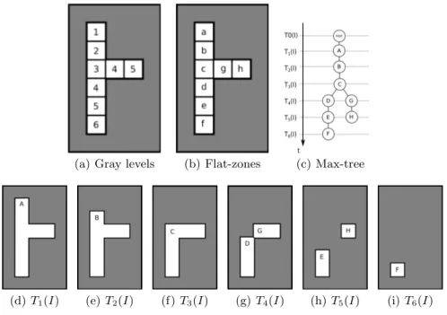
Let us explain the max-tree construction with the toy example of Fig.3. For this example 4-connectivity is used. Consider the image 3(a)containing 8 flat-zones enumerated from a to h (in lower-case letters). Gray regions correspond to zero valued pixels. Figures3(d)to3(i)present the successive thresholds from T1(I) to T6(I), respectively. Fig.3(c)presents the corresponding max-tree built
from those successive thresholds. Note that a given threshold may be composed by several CCs, enumerated from A to H (in upper-case letters). For example, threshold T4(I) has two CCs D and G. Moreover, a CC may be related to
several zones. For example, node D in the max-tree is associated to flat-zones d, e and f in the input image. The max-tree construction starts at the lowest level t=0, corresponding to the root of the tree. The first level is composed by threshold T1(I) containing CC A in Fig.3(d). Threshold T2(I) is composed
by single CC B while T3(I) is composed by C. Following the inclusion rule,
T3(I) ⊆ T2(I) ⊆ T1(I), we add B and C to the main trunk of the tree. Node C
contains two children since threshold T4(I) in Fig.3(g)contains two CCs D and
G. The construction of these two branches is straightforward since F ⊆ E ⊆ D and H ⊆ G.
In addition, it is possible to associate a flat-zone in I to a given node in the tree. Note that a node might be associated to several flat-zones. In fact, a given
(a) Gray levels (b) Flat-zones (c) Max-tree
(d) T1(I) (e) T2(I) (f) T3(I) (g) T4(I) (h) T5(I) (i) T6(I)
Fig. 3. Max-tree construction. The image is composed by 8 flat-zones enumerated from a to h. Each node corresponds to a CC, enumerated from A to H, of threshold Tt(I).
The max-tree contains two leafs corresponding to the two maxima at f and h.
flat-zone at level t is contained in the subset of Tt(I) where gray level is equal
to t in the input image. For example, flat-zone c in Fig.3(b)corresponds to the pixels of C in Fig. 3(f)where the gray level is equal to 3 in the input image : c = {p ∈ C | I(p) = 3}.
In general, several filters can be applied to the tree (i.e. pruning leaves) and the output image is the restitution from the filtered tree. There exist sev-eral filtering rules to recompose the output image from the filtered max-tree [1,14,20,19]. The choice of the filtering rule depends on the application. In this paper, we will focus on the direct rule: all CCs Tt(I) holding a given criterion
are stacked to recompose the output image.
Let us illustrate the filtering process based on max-tree with the example of Fig.4. In this case, we want to filter branches with contrast lower than or equal to 2 (this is equivalent to a h-Maxima filter with h=2). The contrast of a branch is defined as the gray-level difference between the first and the last node of the branch. This leads to remove the nodes G and H in Fig. 4(a). Fig. 4(b) shows the output image recomposed from the filtered max-tree using the direct rule. Fig.4(c)shows the corresponding flat-zones filtered in the process.
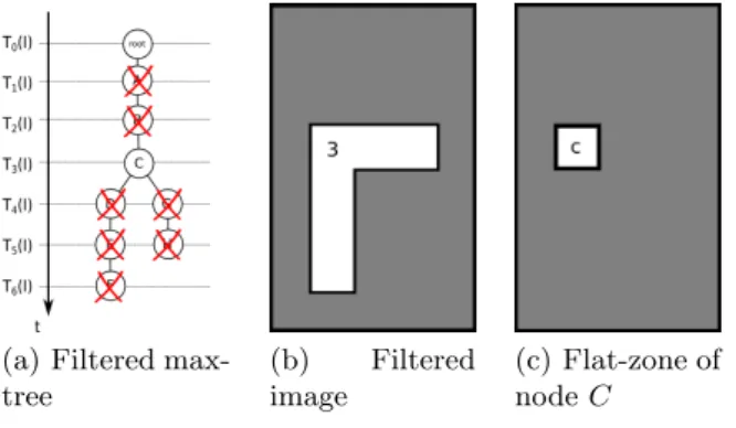
Fig.5 presents another example of image filtering using the max-tree struc-ture. In this case, we want to remove nodes with less than 2 children. This leads to remove all the nodes except C and the root of the tree (see Fig.5(a)). Fig.5(b)
(a) Filtered max-tree (b) Filtered image (c) FZ of nodes G and H
Fig. 4. Max-tree based filtering on image of Fig.3(a). Branches with contrast lower than or equal to 2 are removed. The output image is recomposed from the filtered max-tree using the direct rule. This is equivalent to a h-Maxima filter with h=2.
shows the output image recomposed from the filtered max-tree using the direct rule. Fig.5(c)shows the flat-zone c corresponding to remaining node C.
(a) Filtered max-tree
(b) Filtered image
(c) Flat-zone of node C
Fig. 5. Max-tree based filtering on image of Fig.3(a). Nodes with less than 2 children are removed. Output image is recomposed from the filtered max-tree. Fig.5(c)shows the flat-zone c corresponding to node C in the input image.
3
Finding junction regions
A classic method to find junction regions can be summarized in Fig.6as follows: 1. Compute the skeleton of the input image (Fig. 6(a)). A great number of
2. Ideally, each junction region in the skeleton representation corresponds to an interesting intersection in the input object. In practice, there are often spu-rious junction regions associated to unwanted skeletal branches. If needed, these branches can be removed using a parametric pruning in order to get a clean skeleton (Fig.6(b)).
3. Individual skeletal branches are obtained by suppressing junction regions from the skeleton (magenta points in Fig.6(b)).
4. Junction regions are computed using the skeleton by influence zones (SKIZ) of the remaining skeleton (Fig.6(c)) within the input object.
5. Finally, the SKIZ allows the segmentation in individual branches (Fig.6(d)).
(a) Input object (b) Junctions on skeleton
(c) Junctions on object
(d) Segmented branches
Fig. 6. Extraction of junction regions using a method based on skeletonization.
In general, this classic method works well for thin and clean structures, but may fail on thick objects with bent branches and protrusions. A critical step is the choice of both the appropriate skeletonization algorithm and the pruning strategy in order to keep interesting branches. In several applications, the user is not particularly interested in the skeleton but in the junction regions. Thus, we propose to find junction regions directly on binary objects avoiding skeletoniza-tion. Our method is based on geodesic operators since the wavefronts of the geodesic propagation provide interesting information about junction regions. It is intended to work not only on thin objects but also on elongated structures with possible thick branches, protrusions and noise. Moreover, it provides an intuitive and straightforward way to filter out short branches and protuberances.
Consider a binary object without holes X, a geodesic propagation starting from a geodesic extremity y and a max-tree T built from the geodesic distance function dX(y). Let analyze the object of Fig. 3. In such a case, the
propaga-tion starts from the upper pixel of the object. When the propagapropaga-tion reaches a junction region, the wavefront splits from a single flat-zone c at level t=3 to two separated flat-zones d and g at level t=4. This is represented by a node with two children in the max-tree. It is noteworthy that the flat-zone c, corresponding to node C, is a junction region. Informally, the number of branches in a junction region is equivalent to the number of children at its corresponding node in the max-tree representation. Since nodes with more than one child correspond to
junction regions, we propose the following methodology to find junction regions on a binary object without holes X:
1. Find a geodesic extremity y of object X,
2. Compute the geodesic distance from y inside X, called dX(y),
3. Construct a max-tree T from dX(y),
4. (Optional) Compute a filtered tree T0 by removing branches shorter than h, 5. Compute a filtered tree T00 by removing nodes with less than two children, 6. Junction regions J are obtained as the flat-zones of I corresponding to
re-maining nodes in filtered tree T00,
7. Individual branches B are obtained by removing junction regions J from the object X: B = X\J .
Note that step 4 is optional and equivalent to applying a h-Maxima filter to the geodesic distance function. For the sake of efficiency, this filter can be computed directly on the max-tree by computing the contrast of each branch.
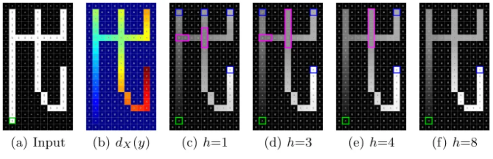
Fig.7 illustrates our proposed method on a synthetic binary object. In this example 8-connectivity is used. The propagation starts from the lower left ex-tremity of the object (green square in Fig. 7(a)). At the beginning, between iteration 1 and 12 in Fig.7(b), each wavefront is composed of a single flat-zone. When the propagation reaches the first bifurcation at iteration 13, the wavefront splits into two separate flat-zones. This bifurcation indicates the presence of a junction region. If we continue to the right of the image, we can see another junction region at iteration 16. In this case, the wavefront splits producing three different flat-zones at value t=17.
It is noteworthy that each maximum in the geodesic distance function corre-sponds to an extremity of the object. As explained in Subsection2.3, the contrast of a branch corresponds to its length. The h-Maxima operator can be used to filter maxima less contrasted than a given threshold h. This is a straightforward way to remove short and spurious extremities. Figures7(c)to 7(f)present four examples of finding junction regions after h-Maxima filtering. Green points indi-cate the initial point of the geodesic distance computation, blue points indiindi-cate the regional maxima, and magenta points indicate the detected junction regions. In Fig.7(c), the geodesic distance function contains four maxima, corresponding to the four extremities of the object (the starting point is of course an extremity, but it is a minimum because it is the starting point of the propagation). The object contains two junction regions at levels t=13 and t=16, respectively. In Fig.7(d), branches shorter than 3 pixels (h-Maxima filter with h=3) are filtered out. Note that the second extremity is not a maximum anymore and has been merged with the junction region. Please note here the impact of the connectivity on the branch length estimation. Although the upper left and the middle spikes of the object seem to have the same length, they are not filtered for the same value of h. If we use 4-connectivity instead of 8-connectivity, both extremities would be filtered at the same value of h. In Fig. 7(e), branches shorter than 4 pixels (h-Maxima filter with h=4) are filtered out. Note that only two extremities are still regional maxima of the image and only one junction region is detected.
Finally, Fig.7(f)shows a h-Maxima filter with h=8. Note that only the longest branch is still a maximum of the geodesic distance function. In this case, no junction regions are extracted.
(a) Input (b) dX(y) (c) h=1 (d) h=3 (e) h=4 (f) h=8
Fig. 7. Junction regions on an object without holes. Green point indicates the initial seed of the geodesic distance, blue points indicate the regional maxima, and magenta points indicate the detected junction regions for several h parameters.
4
Results
To evaluate our method, we present three tests on synthetic and real images. Our method is qualitatively compared to a classic method based on skeletonization (explained in Section3). In order to make a fair comparison, the classical method is based on a “perfect” hand-made skeleton.
Fig. 8 illustrates an example of detection of junction regions on a binary object containing thin and thick branches. Fig. 8(c) presents the result using a classic method based on skeletonization. Fig. 8(d) presents the result of our proposed method. In both methods, branches shorter than 30 pixels have been filtered out. Note that our method is able to manage thick objects and the filtering strategy to remove non interesting branches is intrinsically taken into account in the max-tree representation. Note also that both methods are able to extract correctly the five junction regions, generating 10 individual branches. However, our method does not require any skeleton computation.
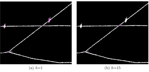
Fig.9illustrates a real top-view image of electric cables in a railway environ-ment. Cables are interconnected at several locations. The goal is to segment the image into individual cable segments. Fig.9(b)presents the segmentation result with our geodesic method considering all geodesic extremities (h=1). Note that several junction regions are extracted due to short protrusions in the image. In fact, those protrusions correspond to cable insulators. In order to filter out these insulators, the segmentation is carried out considering only branches longer than 15 pixels, as shown in Fig.9(c).
(a) Input (b) Geodesic dis-tance (c) Method based on skeletonization (d) Our geodesic method
Fig. 8. Junction regions using a classical method based on skeletonization and our proposed method. In both methods, branches shorter than 30 pixels are filtered out.
(a) Input image (b) h=1 (c) h=15
Fig. 9. Segmentation of individual electric cables on a railway environment. Junction regions are extracted with our proposed geodesic method using two different h param-eters. Each color represents an individual cable.
Fig. 10 presents another example of electric cables in a railway environ-ment. Fig. 10(a) presents the junction regions considering all branches (h=1). Fig.10(b)presents the junction regions considering only branches longer than 15 pixels (h=15). In this case, cable insulators are not detected as junction regions, resulting in a correct segmentation of individual cables.
5
Conclusions and perspectives
We have proposed a method to find junction regions in objects without holes based on geodesic operators. In particular, our method is based on the analysis
(a) h=1 (b) h=15
Fig. 10. Segmentation of individual electric cables on a railway environment. Two different h parameters have been used.
of the wavefront evolution in a geodesic propagation. Our method is generic and does not require skeletonization. It provides an intuitive and straightforward way to filter short extremities and protuberances. Moreover, an elegant and efficient implementation using a max-tree representation is proposed.
The problem with objects with holes is that the basic hypothesis: “the max-ima on the geodesic distance correspond to the extremities of the object” does not hold anymore. In fact, a loop introduces the union of wavefronts coming from different branches, which introduces additional maxima on the geodesic distance function. We are currently working in a more generic method to extract junction regions on any binary object. The key step of such a method is replacing the max-tree structure by a more generic geodesic graph.
References
1. E. J. Breen and R. Jones. Attribute openings, thinnings, and granulometries. Computer Vision and Image Understanding, 64(3):377–389, 1996.
2. J. Chaussard. Topological tools for discrete shape analysis. PhD thesis, Universit´e Paris-Est, dec 2010.
3. J. Chaussard, M. Couprie, and H. Talbot. Robust skeletonization using the discrete lambda-medial axis. Pattern Recognition Letters, 32(9):1384–1394, 7 2011. 4. J. Fabrizio and B. Marcotegui. Fast implementation of the ultimate opening.
ISMM09, 9th International Symposium on Mathematical Morphology, pages 272– 281, 2009. Groningen, The Netherlands.
5. L. Garrido, A. Oliveras, and P. Salembier. Motion analysis of image sequences using connected operators. Proceedings of SPIE - The International Society for Optical Engineering, 3024:546–557, 01 1997.
6. S. B. Gray. Local Properties of Binary Images in Two Dimensions. IEEE Trans-actions on Computers, C-20(5):551–561, may 1971.
7. W. H. Hesselink, M. Visser, and J. B. T. M. Roerdink. Euclidean Skeletons of 3D Data Sets in Linear Time by the Integer Medial Axis Transform. In Mathematical Morphology: 40 Years On, pages 259–268, Dordrecht, 2005. Springer Netherlands. 8. R. Kimmel, D. Shaked, N. Kiryati, and A. M. Bruckstein. Skeletonization via Dis-tance Maps and Level Sets. Computer Vision and Image Understanding, 62(3):382– 391, 1995.
9. C. Lantu´ejoul. Skeletonization in quantitative metallography, volume 34, pages 107–135. Sijthoff and Noordhoff, 1980.
10. C. Lantu´ejoul and S. Beucher. On the use of the geodesic metric in image analysis. Journal of Microscopy, 121(1):39–49, 1981.
11. V. Morard, E. Decenci`ere, and P. Dokl´adal. Geodesic Attributes Thinnings and Thickenings Background : Attribute Thinnings. In ISMM’11, 10th international conference on Mathematical morphology, pages 200–211, 2011.
12. V. Morard, E. Decenci`ere, and P. Dokl´adal. Efficient geodesic attribute thinnings based on the barycentric diameter. Journal of Mathematical Imaging and Vision, 46(1):128–142, 2013.
13. L. Najman and M. Couprie. Building the Component Tree in Quasi-Linear Time. IEEE Transactions on Image Processing, 15(11):3531–3539, 2006.
14. P. Salembier, A. Oliveras, and L. Garrido. Anti-extensive connected operators for image and sequence processing. IEEE Transactions on Image Processing, 7(4):555– 570, 04 1998.
15. P. Salembier and J. Serra. Flat zones filtering, connected operators, and filters by reconstruction. IEEE Transactions on Image Processing, 4:1153–1160, 1995. 16. J. Serra. Image analysis and mathematical morphology, volume 1. Academic Press,
Orlando, FL, USA, 1982.
17. J. Serra. Image Analysis and Mathematical Morphology: Theoretical Advance, vol-ume 2. Academic Press, 1988.
18. P. Soille. Morphological Image Analysis: Principles and Applications. Springer-Verlag, Secaucus, NJ, USA, 2003.
19. E. R. Urbach, J. B. T. M. Roerdink, and M. H. F. Wilkinson. Connected Shape-Size Pattern Spectra for Rotation and Scale-Invariant Classification of Gray-Scale Im-ages. IEEE Transactions on Pattern Analysis and Machine Intelligence, 29(2):272– 285, 2007.
20. E. R. Urbach and M. H. F. Wilkinson. Shape-Only Granulometries and Gray-Scale Shape Filters. In ISMM’02, 8th International Symposium on Mathematical Morphology, pages 305–314, 2002.
21. L. Vincent. Efficient computation of various types of skeletons. In Medical Imaging V: Image Processing, volume 1445, pages 297–312. International Society for Optics and Photonics, 1991.
22. L. Vincent. Morphological grayscale reconstruction in image analysis: efficient algorithms and applications. IEEE Transactions on Image Processing, 2:176–201, 1993.
23. X. Huang and M. Fisher and D. J. Smith. An Efficient Implementation of Max Tree with Linked List and Hash Table. In DICTA, 2003.