HAL Id: tel-01347050
https://pastel.archives-ouvertes.fr/tel-01347050
Submitted on 20 Jul 2016
HAL is a multi-disciplinary open access archive for the deposit and dissemination of sci-entific research documents, whether they are pub-lished or not. The documents may come from teaching and research institutions in France or abroad, or from public or private research centers.
L’archive ouverte pluridisciplinaire HAL, est destinée au dépôt et à la diffusion de documents scientifiques de niveau recherche, publiés ou non, émanant des établissements d’enseignement et de recherche français ou étrangers, des laboratoires publics ou privés.
financial valuations area
Jose Arturo Infante Acevedo
To cite this version:
Jose Arturo Infante Acevedo. Numerical methods and models in market risk and financial valuations area. General Mathematics [math.GM]. Université Paris-Est, 2013. English. �NNT : 2013PEST1086�. �tel-01347050�
THÈSE
présentée pour l’obtention du titre de
Docteur de l’Université Paris-Est
Spécialité : Mathématiques Appliquéespar
José Arturo Infante Acevedo
Ecole Doctorale :Mathématiques et Sciences et Technologies de l’Information et de la Communication
Méthodes et modèles numériques appliqués
aux risques du marché et à l’évaluation
financière
Soutenue le XX XX 2013 devant le jury composé de :
Rapporteurs : Frédéric Abergel Yves Achdou
Président : Bernard Lapeyre
Examinateur : Mohamed Baccouche
Directeurs de thèse : Aurélien Alfonsi Tony Lelièvre
Méthodes et modèles numériques appliqués aux risques du marché et à l’évaluation financière
Ce travail de thèse aborde deux sujets : (i) L’utilisation d’une nouvelle méthode numérique pour l’évaluation des options sur un panier d’actifs, (ii) Le risque de liquidité, la modélisation du carnet d’ordres et la microstructure de marché.
Premier thème : Un algorithme glouton et ses applications pour résoudre des équa-tions aux dérivées partielles
Beaucoup de problèmes d’intérêt dans différents domaines (sciences des matériaux, finance, etc) font intervenir des équations aux dérivées partielles (EDP) en grande dimension. L’exemple typique en finance est l’évaluation d’une option sur un panier d’actifs, laquelle peut être obtenue en résolvant l’EDP de Black-Scholes ayant comme dimension le nombre d’actifs considérés. Nous proposons d’é-tudier un algorithme qui a été proposé et étudié récemment dans [ACKM06, BLM09] pour résoudre des problèmes en grande dimension et essayer de contourner la malédiction de la dimension. L’idée est de représenter la solution comme une somme de produits tensoriels et de calculer itérativement les termes de cette somme en utilisant un algorithme glouton. La résolution des EDP en grande di-mension est fortement liée à la représentation des fonctions en grande didi-mension. Dans le Chapitre 1, nous décrivons différentes approches pour représenter des fonctions en grande dimension et nous introduisons les problèmes en grande dimension en finance qui sont traités dans ce travail de thèse.
La méthode sélectionnée dans ce manuscrit est une méthode d’approximation non-linéaire ap-pelée Proper Generalized Decomposition (PGD). Le Chapitre 2 montre l’application de cette méthode pour l’approximation de la solution d’une EDP linéaire (le problème de Poisson) et pour l’approxima-tion d’une foncl’approxima-tion de carré intégrable par une somme des produits tensoriels. Un étude numérique de ce dernier problème est présenté dans le Chapitre 3. Le problème de Poisson et celui de l’approxima-tion d’une foncl’approxima-tion de carré intégrable serviront de base dans le Chapitre 4 pour résoudre l’équal’approxima-tion de Black-Scholes en utilisant l’approche PGD. Dans des exemples numériques, nous avons obtenu des résultats jusqu’en dimension 10.
Outre l’approximation de la solution de l’équation de Black-Scholes, nous proposons une méthode de réduction de variance des méthodes Monte Carlo classiques pour évaluer des options financières.
Second thème : Risque de liquidité, modélisation du carnet d’ordres, microstructure de marché
Le risque de liquidité et la microstructure de marché sont devenus des sujets très importants dans les mathématiques financières. La dérégulation des marchés financiers et la compétition entre eux pour attirer plus d’investisseurs constituent une des raisons possibles. Les règles de cotation sont
savoir à chaque instant le nombre d’ordres en attente pour certains actifs et d’avoir un historique de toutes les transactions passées. Dans ce travail, nous étudions comment utiliser cette information pour exécuter de facon optimale la vente ou l’achat des ordres. Ceci est lié au comportement des traders qui veulent minimiser leurs coûts de transaction.
La structure du carnet d’ordres (Limit Order Book) est très complexe. Les ordres peuvent seulement être placés dans une grille des prix. A chaque instant, le nombre d’ordres en attente d’achat (ou vente) pour chaque prix est enregistré. Pour un prix donné, quand deux ordres se correspondent, ils sont exécutés selon une règle First In First Out. Ainsi, à cause de cette complexité, un modèle exhaustif du carnet d’ordres peut ne pas nous amener à un modèle où, par exemple, il pourrait être difficile de tirer des conclusions sur la stratégie optimale du trader. Nous devons donc proposer des modèles qui puissent capturer les caractéristiques les plus importantes de la structure du carnet d’ordres tout en restant possible d’obtenir des résultats analytiques.
Dans [AFS10], Alfonsi, Fruth et Schied ont proposé un modèle simple du carnet d’ordres. Dans ce modèle, il est possible de trouver explicitement la stratégie optimale pour acheter (ou vendre) une quantité donnée d’actions avant une maturité. L’idée est de diviser l’ordre d’achat (ou de vente) dans d’autres ordres plus petits afin de trouver l’équilibre entre l’acquisition des nouveaux ordres et leur prix.
Ce travail de thèse se concentre sur une extension du modèle du carnet d’ordres introduit par Alfonsi, Fruth et Schied. Ici, l’originalité est de permettre à la profondeur du carnet d’ordres de dépendre du temps, ce qui représente une nouvelle caractéristique du carnet d’ordres qui a été illustré par [JJ88, GM92, HH95, KW96]. Dans ce cadre, nous résolvons le problème de l’exécution optimale pour des stratégies discrétes et continues. Ceci nous donne, en particulier, des conditions suffisantes pour exclure les manipulations des prix au sens de Huberman et Stanzl [HS04] ou de Transaction-Triggered Price Manipulation (voir Alfonsi, Schied et Slynko). Ces conditions nous donnent des intu-itions qualitatives sur la manière dont les teneurs de marché (market makers) peuvent créer ou pas des manipulations des prix.
Numerical methods and models in market risk and financial valuations area
This work is organized in two themes : (i) A novel numerical method to price options on many assets, (ii) The liquidity risk, the limit order book modeling and the market microstructure.
First theme : Greedy algorithms and applications for solving partial differential equations in high dimension
Many problems of interest for various applications (material sciences, finance, etc) involve high-dimensional partial differential equations (PDEs). The typical example in finance is the pricing of a basket option, which can be obtained by solving the Black-Scholes PDE with dimension the number of underlying assets. We propose to investigate an algorithm which has been recently proposed and ana-lyzed in [ACKM06, BLM09] to solve such problems and try to circumvent the curse of dimensionality. The idea is to represent the solution as a sum of tensor products and to compute iteratively the terms of this sum using a greedy algorithm. The resolution of high dimensional partial differential equations is highly related to the representation of high dimensional functions. In Chapter 1, we describe various linear approaches existing in literature to represent high dimensional functions and we introduce the high dimensional problems in finance that we will address in this work.
The method studied in this manuscript is a non-linear approximation method called the Proper Generalized Decomposition. Chapter 2 shows the application of this method to approximate the so-lution of a linear PDE (the Poisson problem) and also to approximate a square integrable function by a sum of tensor products. A numerical study of this last problem is presented in Chapter 3. The Poisson problem and the approximation of a square integrable function will serve as basis in Chapter 4 for solving the Black-Scholes equation using the PGD approach. In numerical experiments, we obtain results for up to 10 underlyings.
Besides the approximation of the solution to the Black-Scholes equation, we propose a variance reduction method, which permits an important reduction of the variance of the Monte Carlo method for option pricing.
Second theme : Liquidity risk, limit order book modeling and market microstructure Liquidity risk and market microstructure have become in the past years an important topic in mathematical finance. One possible reason is the deregulation of markets and the competition between them to try to attract as many investors as possible. Thus, quotation rules are changing and, in general, more information is available. In particular, it is possible to know at each time the awaiting orders on some stocks and to have a record of all the past transactions. In this work we study how to use this information to optimally execute buy or sell orders, which is linked to the traders’ behaviour that want to minimize their trading cost.
grid. At each time, the number of waiting buy (or sell) orders for each price is stored. For a given price, orders are executed according to the First In First Out rule, as soon as two orders match together. Thus, since it is really complex, an exhaustive modeling of the LOB dynamics would not lead, for example, to draw conclusions on an optimal trading strategy. One has therefore to propose models that can grasp important features of the LOB structure but that allow to find analytical results.
In [AFS10], Alfonsi, Fruth and Schied have proposed a simple LOB model. In this model, it is possible to explicitly derive the optimal strategy for buying (or selling) a given amount of shares before a given deadline. Basically, one has to split the large buy (or sell) order into smaller ones in order to find the best trade-off between attracting new orders and the price of the orders.
Here, we focus on an extension of the Limit Order Book (LOB) model with general shape in-troduced by Alfonsi, Fruth and Schied. The additional feature is a time-varying LOB depth that represents a new feature of the LOB highlighted in [JJ88, GM92, HH95, KW96]. We solve the op-timal execution problem in this framework for both discrete and continuous time strategies. This gives in particular sufficient conditions to exclude Price Manipulations in the sense of Huberman and Stanzl [HS04] or Transaction-Triggered Price Manipulations (see Alfonsi, Schied and Slynko). These conditions give interesting qualitative insights on how market makers may create price manipulations.
Contents
Part I Greedy algorithms and application for solving high-dimensional partial differential equations
1 Approximation of high-dimensional functions and the pricing problem . . . 3
1.1 The curse of dimensionality . . . 3
1.2 Some approaches to approximate high-dimensional functions . . . 4
1.2.1 Sparse grids . . . 5
1.2.2 Canonical, Tucker and Tensor Train decompositions . . . 9
1.3 High-dimensional problems in finance . . . 11
1.3.1 Important concepts in finance . . . 11
1.3.2 The Black-Scholes model . . . 13
1.3.3 High-dimensional partial differential equations in finance . . . 17
2 A nonlinear approximation method for solving high-dimensional partial differential equations. . . 21
2.1 Greedy algorithms . . . 22
2.2 The Proper Generalized Decomposition . . . 25
2.3 Some particular cases: the Singular Value Decomposition and the general linear case . . . 27
2.3.1 Tensor product of spaces . . . 27
2.3.2 The Singular Value Decomposition case . . . 28
2.5 The Proper Generalized Decomposition for the approximation of a square-integrable
function . . . 31
2.6 The Proper Generalized Decomposition in the case of the Poisson problem . . . 33
3 Approximation of a Put payoff function using the Proper Generalized Decomposition . . . 37
3.1 Separated representation of a Put payoff . . . 37
3.2 Fixed point procedure . . . 38
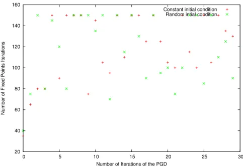
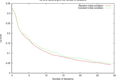
3.3 Initial condition for the fixed point procedure and for the convergence of the Proper Generalized Decomposition method . . . 41
3.4 Criteria of convergence used in practice . . . 42
3.5 Numerical integration . . . 44
3.6 Numerical results . . . 45
3.7 Mass lumping technique . . . 46
3.8 Pricing of a basket put using the separated approximation of the payoff . . . 50
4 Application in Finance of a nonlinear approximation method for solving high-dimensional partial differential equations. . . 53
4.1 The Proper Generalized Decomposition applied to the Black-Scholes partial differential equation . . . 53
4.1.1 Weak formulation of the Black-Scholes partial differential equation . . . 53
4.1.2 Formulation on a bounded domain . . . 56
4.1.3 The IMEX scheme and the Black-Scholes equation as a minimization problem . . . 58
4.1.4 Stability analysis for the IMEX scheme . . . 60
4.1.5 Implementation of the Proper Generalized Decomposition techniques for the Black-Scholes partial differential equation . . . 62
4.2 Numerical results . . . 64
4.2.1 Testing the method against an analytical solution . . . 64
4.2.3 Application as a variance reduction method . . . 67
4.3 Appendix: Formulas for the matrices used to solve the Black-Scholes partial differential equation . . . 69
5 Perspectives of the application of the Proper Generalized Decomposition method for option pricing. . . 73
5.1 Pricing using the characteristic function, application to Bermudan options . . . 73
5.2 The problem of the American options . . . 75
Part II Liquidity risk, limit order book modeling and market microstructure 6 Survey on market impact models . . . 79
6.1 Introduction . . . 79
6.2 Market impact models . . . 82
6.2.1 Definition of the optimal execution problem . . . 82
6.2.2 First family of models (immediate and permanent price impact) . . . 84
6.2.3 Second family of models (transient price impact) . . . 88
6.2.4 Other models . . . 92
6.2.5 A first extension of the second family of models . . . 93
6.2.6 Differences between the Gatheral model and the Alfonsi, Fruth and Schied model 96 6.2.7 Price manipulation strategies . . . 97
6.3 Motivation for our work . . . 98
7 Optimal execution and price manipulations in time-varying limit order books. . . 101
7.1 Market model and the optimal execution problem . . . 103
7.1.1 The model description . . . 103
7.1.2 The optimal execution problem, and price manipulation strategies . . . 105
7.2 Main results . . . 108
7.2.3 Numerical results . . . 121
7.3 Proofs . . . 123
7.3.1 The block shape case . . . 123
7.3.2 General limit order book shape with model V . . . 123
7.3.3 General limit order book shape with model P . . . 129
Part I
Greedy algorithms and application for solving high-dimensional
partial differential equations
1
Approximation of high-dimensional functions and the pricing
problem
The approximation of high-dimensional functions is an important subject because of the large domain of applications.
The main difficulty for approximating high-dimensional functions is that when the dimension increases, the quantity of information increases exponentially fast with the dimension. This obstacle is known as the curse of dimensionality.
In Section 1.2, we present different approaches proposed in the literature for representing high-dimensional functions. In particular, in Section 1.2, we discuss the linear techniques, the non-linear methods being defined in Chapter 2. We draw your attention on the fact that the non-linear techniques will be the methods used in this manuscript.
Before introducing these linear methods to approximate high-dimensional functions, let us dis-cuss the curse of dimensionality in order to understand the difficulties behind the study of high-dimensional problems.
1.1 The curse of dimensionality
Let us introduce the Hilbert space V. The main idea of the deterministic approaches is to represent solutions u ∈ V as linear combinations of tensor products. The approximation by a full tensor products writes:
u(x1, x2. . . , xd) = N1 � i1=1 N2 � i2=1 . . . Nd � id=1 ui1i2...idφ i1(x1)φi2(x2) . . . φid(xd) (1.1)
where ui1i2...id ∈ R for all i
j = 0, . . . Nj, j = 1, . . . , d and �
φij
�
1≤ij≤Nj
are the basis of the vector spaces of dimension Nj for all j = 1, . . . , d which are fixed. As a consequence, this approach leads to
N =
d � j=1
Nj (1.2)
that grows exponentially in terms of the dimension d.
The following result given by DeVore, Howard and Micchelli [DHM89] allows to see in practice the curse of dimensionality because it shows that a sampling method cannot do better than a certain error estimate depending exponentially on the dimension.
This result is based on the non-linear manifold width. Let X be a normed space and K ⊂ X a compact set. Let us consider the maps E : K �→ RN for the encoding and R : RN �→ X for the
reconstruction. Introducing the distortion of the pair (E, R) over K max
u∈K �u − R(E(u))�X,
we define the non-linear N-width of K as dN(K) := inf
E,Rmaxu∈K �u − R(E(u))�X
where the infimum is taken over all the continuous maps (E, R). If X = L∞and K is the unit ball of
Cm([0, 1]d), it can be proven that (see [DHM89])
cN−md ≤ dN(K) ≤ CN− m
d
where c and C are two constant that do not depend on N. For a fixed error level, the number of degrees of freedom grows exponentially fast with the dimension. In conclusion, for high-dimensional problems, appropriate approximation tools should be studied.
In this direction, we present in the following Section 1.2 approximation methods that allow to reduce the number of degree of freedom given the tensorial form of their approximated solutions.
1.2 Some approaches to approximate high-dimensional functions
In this section, we present a short survey on methods proposed in the literature for approx-imating high-dimensional functions. We recall that the approach used in this work to obtain this approximations is presented in Chapter 2.
1.2 Some approaches to approximate high-dimensional functions 5
1.2.1 Sparse grids
The sparse grid method is a numerical discretization technique for multivariate problems. This approach is introduced in [Smo63] and studied by Schwab [PS04] and Zenger [Zen91]. In this part, we present a short survey of this method. See [BG04] for a complete introduction to the sparse grid methods. This approach is also known under the name of hyperbolic cross points or splitting interpolations.
Let us consider X = [0, 1]. The use of one-dimensional multilevel (or hierarchical) basis is one of the main ideas of the sparse grid method. In the classical approach, the following standard hat function is employed to construct the hierarchical basis functions
φ(ξ) := 1 − |ξ|, if ξ ∈ [−1, 1] 0, otherwise. (1.3)
Consequently, we can consider a set of equidistant grids of level m and mesh width hm = 2−m
on X by introducing the following points:
ξm,i:= i2−m, 0≤ i ≤ 2m.
Associated to the points ξm,i, we define the basis function (φm,i)1≤i≤2m−1 using the standard
hat function (1.3) φm,i(x) := φ �x− x m,i 2−m � .
We note that this basis is the standard basis of P1 Lagrange finite element functions with mesh
size hm and with support on [ξm,i− hm, ξm,i+ hm].
Thus, we can define the function spaces
Vm := Span {φm,i, 1≤ i ≤ 2m− 1}
and the hierarchical increment spaces Wm
Wm:= Span {φm,i, i∈ Im} ,
Im:= {i ∈ N, 1 ≤ i ≤ 2m− 1, i odd } .
Hence, the increment spaces verify the following relation
Vm= �
k≤m
Wk,
where the symbol ⊕ means that the sum is direct. This decomposition (φi,k)k≤m,i∈Ik leads to the
hierarchical basis of Vm because any continuous piecewise linear function u ∈ Vm can be written as
u = m � k=1 � i∈Ik uk,iφk,i,
with uk,i∈ R for all 1 ≤ k ≤ m and i ∈ Ik. We remark that the support of all the basis functions φk,i
spanning Wk are mutually disjoint.
In order to explain, the tensor product construction in high-dimensional spaces, let us introduce i = (i1, . . . , id) ∈ Nd and k = (k1, . . . , kd) ∈ Nd two multi-indices. The notation
i≤ k
means that
∀ 1 ≤ j ≤ d, ij ≤ kj
Moreover, we will consider the notation 2i= (2i1, . . . , 2id) ∈ Nd and 1 = (1, . . . , 1) ∈ Np.
The goal is to construct a multi-dimensional basis on Xd= [0, 1]dfrom the one-dimensional
hier-archical basis. In order to do that, we consider the d-dimensional tensorization of the one-dimensional basis (φk,i)1≤k≤m,i∈Ik by introducing m = (m1, . . . , md) the multi-index denoting the level of
dis-cretization in each dimension and the grid points xm,i given by
xm,i = (xm1,i1, . . . , xmd,id)
where i = (i1, . . . , id) ∈ Nd with 1 ≤ i ≤ 2m.
Then, for each grid point xm,i, an associated d-dimensional basis function φm,i is defined as the
1.2 Some approaches to approximate high-dimensional functions 7 φm,i(x1, . . . , xd) := d � j=1 φmj,ij(xj).
Thus, using this basis of functions, we can define the spaces Vm of continuous piecewise d-linear
functions
Vm := Span {φm,i, 1≤ i ≤ 2m− 1} . (1.4)
As in the one-dimensional case, we can define the hierarchical increments Wm as follows
Wm := Span {φm,i, i∈ Im}
where Im := �
i∈ Nd, 1≤ i ≤ 2m− 1, i
j odd for all 1 ≤ j ≤ d �
Consequently, the spaces Vm verify the property
Vm= �
k≤m
Wk,
and therefore any function u ∈ Vm can be written under the form
u(x) = �
1≤k≤m �
i∈Ik
uk,iφk,i(x), uk,i∈ R.
In order to introduce an optimization with respect to the number of degrees of freedom and the obtained accuracy of the approximation, we consider the sparse grid space ˆVn of level n defined as
follows: ˆ Vn:= � |k|1≤n+d−1 Wk.
where |k|1 and |k|∞ are two norms for multi-indices k = (k1, . . . , kd) ∈ Nd such that
|k|1 := d � j=1 |kj| and |k|∞:= max 1≤j≤d|kj|,
moreover, in this case, the associated full grid space Vncan be written as
Vn:= �
|k|∞≤n
The dimension of the space ˆVn, that means, the number of degrees of freedom or grid points is given by dim ˆVn= n−1 � i=0 2i � p− 1 + i p− 1 � = O(h−1 n | log2(hn)|p−1).
We remark that the space Vncan be seen as the discretization space associated with a standard
P1 finite element discretization based on a uniform discretization of mesh size hn = 2−n, so the dimension of the space Vn is of the order O(h−pn ). Consequently, the reduction in the number of
degrees of freedom is significant by considering ˆVn instead of Vn.
To show the accuracy of the approximation obtained by the sparse grid methods, we introduce the following Sobolev space
H2,mix(Xd) :=�u∈ L2(Xd), ∂αu∈ L2(Xd), α ∈ Nd,|α|
∞≤ 2
�
,
and we denote by ΠVn and ΠVˆn, the L2(Xd)-orthogonal projector of L2(Xd) onto Vn and onto ˆVn
respectively.
For all u ∈ H2,mix(Xd) ∩ H1
0(Xd), the approximation error of the function u on the sparse grid
space is
�u − ΠVˆnu�L2(Xd)= O(h2nnd−1), (1.5)
and on the full grid space, the accuracy is
�u − ΠVnu�L2(Xd)= O(h 2
n). (1.6)
For a given error level, in (1.5), the number of degrees of freedom does not grow exponentially with the dimension. These results (see [BG04]) show the advantage of using the sparse grid space ˆVn
with respect to the full grid space Vn because the number of degrees of freedom is strongly reduced
while the accuracy is insignificantly deteriorated if the exact solution is regular enough. The efficiency of the sparse tensor products is lost when the solution u is not regular or when the considered mesh is complicated. Consequently, in practice, this method may be difficult to apply for reasons such as the lack of regularity of the solution and the difficulty to implement the associated algorithms.
1.2 Some approaches to approximate high-dimensional functions 9
1.2.2 Canonical, Tucker and Tensor Train decompositions
In this section, we suppose that the Hilbert space V has the following form:
V =
d �
i=1
Vi. (1.7)
i.e., V is tensor product of Hilbert spaces of univariate functions. In other words, for all 1 ≤ i ≤ d, the function ui ∈ Vi is such that ui : xi ∈ Ωi �→ u(xi) and then a function u ∈ V is such that
u : (x1, . . . , xd) ∈ Ω1× . . . × Ωd�→ u(x1, . . . , xd). By considering (1.7), the goal is to obtain a number
of degrees of freedom which does not depend exponentially on the dimension d.
Canonical decomposition
The canonical decomposition is a classical method to represent in a tensor format a function u∈ V . This approach looks for a representation of u as follows
(x1, . . . , xd) �→ u(x1, . . . , xd) = r � k=1 � d � i=1 ui,k � (x1, . . . , xd), (1.8)
that is, u is represented by r elementary products of single-variate functions. The number r of products of single-variate functions is called the canonical rank of the function u. In a finite dimensional case with dim(Vi) = N, for all i = 1, . . . , d, we can deduce that the complexity of the decomposition (1.8)
is rdN.
Nevertheless, one disadvantage of this approach is that the set of rank-r tensors
Cr := � u∈ V, u(x1, . . . , xd) = r � k=1 � d � i=1 ui,k � (x1, . . . , xd), ∀1 ≤ r, ui,k∈ Vi �
is not a weakly closed subset of V when d ≥ 3 and r ≥ 2, see [dSL08]. Consequently, there may not exists a minimizer to the problem
inf
˜
u∈Cr�u − ˜u� V
Tucker decomposition
A more robust tensor format decomposition is called the Tucker decomposition that consists in decomposing u as follows: (x1, . . . , xd) �→ u(x1, x2, . . . , xd) = r1 � k1=1 . . . rd � kd=1 ck1,...,kd � p � i=1 ui,ki � (x1, . . . , xp),
where for all 1 ≤ i ≤ d, ri∈ N∗, ui,ki ∈ Vi for all 1 ≤ ki≤ ri and ck1,...,kp∈ R.
Thus, in the Tucker decomposition, the function u is decomposed over all the possible tensor products between the functions (ui,ki)1≤kiri for all 1 ≤ i ≤ d.
Let us note rT := (r1, . . . , rp) ∈ (N∗)p the Tucker rank of u. The set of tensors of Tucker rank
rT is weakly closed in V , then the problem of the best approximation has a solution. Nevertheless, we
observe that if rT = (r, . . . , r) and dimVi = N for all 1 ≤ i ≤ d this approach leads to a complexity
given by O(rd+ Nrd) that is exponential with the respect to the dimension d. Hence, the Tucker
decomposition is not pertinent when d is large.
Tensor train
The following decomposition allows to overcome the exponential complexity obtained in the case of the Tucker decomposition and it is called tensor train decomposition. In this case, the function u is represented as follows: (x1, . . . , xd) �→ u(x1, . . . , xd) = r1 � k1=1 . . . rd−1 � kd−1=1 U1(x1, k1)U2(k1, x2, k2) . . . Ud−1(kd−2, xd−1, kd−1)Up(kd−1, xd).
The rank of the function u in the case of the tensor train is defined as rT T = (r1, . . . , rd−1) ∈
(N)d−1. Based on this tensor train decomposition, a function u can be expressed as the following
product of matrices
u(x1, . . . , xd) = U1(x1) . . . Up(xp)
1.3 High-dimensional problems in finance 11 x1 �→ U1(x1) ∈ R1×r1, x2 �→ U2(x2) ∈ Rr1×r2, . . . xd−1�→ Ud−1(xd−1)Rrd−2×rd−1, xd�→ Ud(xd) ∈ Rrd−1×1.
The set of functions of tensor train rank of at most rT T is a weakly closed subset of V. Moreover,
the complexity of this type of decomposition is O(r2N d) if r
i = r and dimVi = N for all i = 1, . . . d
and not exponential with respect to d as in the case of the Tucker decomposition.
The algorithms used in practice to compute the best approximation of a given tensor in the Tucker or tensor train format, execute successive Singular Value Decomposition problems. We can men-tion the Higher Order Orthogonal Iteramen-tion (HOOI) [LMV00a], the Newton-Grassman approach [ES09] or the Higher Order Singular Value Decomposition (HOSVD) [LMV00b].
1.3 High-dimensional problems in finance
In finance, many of the high-dimensional applications include high-dimensional partial differen-tial equations (PDE). A high-dimensional PDE is an equation that depends on several independent variables. Roughly, the PDEs can be classified in elliptic, parabolic and hyperbolic. In this work, we principally study the parabolic ones, given that in finance the relation between the Black-Scholes model (see Section 1.3.2) and this type of equations give them a strong importance.
The goal of this section is to present some high-dimensional PDEs that appear in finance and that are studied in this manuscript, but before that, it is important to begin by introducing the standard framework used in mathematical finance.
1.3.1 Important concepts in finance
The pricing of financial options is one of the most important problems in financial mathematics. In 1900, Bachelier [Bacal] is the first that shows that for answering this kind of problems it is important to use suitable mathematical techniques. This domain did not have a very strong development until the 70’s with the Black-Scholes model developed in 1973 by Merton, Black and Scholes [Mer76, BS73], where they define the price of derivatives as the price needed to hedge them. After that, the financial mathematics domain was driven by the martingale theory developed in the 80’s.
One of the most typical examples of derivatives proposed in markets are the options. An Eu-ropean call (resp. put) option is a financial contract that gives to the holder the option and not the
obligation to buy (resp. sell) a number of stocks to the price K at time T . The fixed price K is known as the strike and T is the maturity of the option. The underlying is equal to ST at the maturity T and
the option will be exercised if ST > K (resp. ST < K) and consequently, the holder’s gain is given by
ST − K (resp. K − ST) because he can buy (resp. sell) the stock at the price K and after sell (resp.
buy) it in the market at the price ST. Otherwise, the option is not exercised and the gain is equal to
0. Hence, we note that the value of the call at the maturity is given by
(ST − K)+= max(ST − K, 0).
For the counterpart (the bank) which sells the European call option, the goal is to provide the stocks at price K and thus to obtain at the maturity a wealth equal to (ST − K)+. At the time when
the option is sold, the value of the asset ST is not known and then the question of the pricing, that
is, how much the client has to pay to get a call option, is very important.
To answer the question of the pricing, some assumptions are usually considered. The hypothesis that appears in most models is that in a liquid market there is no arbitrage, that means, it is impossible to make profit without taking risks.
Under the assumption of no arbitrage, the price of the call option at time T is given by (ST−K)+.
In general, the price at the maturity of an option is a function of ST called the payoff. There exist
different types of payoff functions,
1∀t∈[0,T ],St∈[a,b]φ(ST), for barrier options,
φ(ST, AT), where At=
1 t
� t
0
Sudu, for options on the average,
φ(ST1, ST2, . . . , STd), for a basket option,
In this work, we will mainly consider the payoff:
φ(ST1, . . . , STd) = � K− 1 d d � i=1 STi � + (1.9)
called a basket put option.
Hence, the function φ depends on d different assets which, in general, do not evolve indepen-dently.
1.3 High-dimensional problems in finance 13
1.3.2 The Black-Scholes model
In section 1.3.1, we already presented the main ideas of the theory of options in the framework of financial mathematics. The goal of this section is to develop the relationship between theory and mathematical equations that are obtained based on the Black-Scholes model.
A partial differential equation for the option pricing problem
In this section, we present the framework that allows to find a PDE for pricing European options. In order to do that, we introduce the classical Black-Scholes model that takes into account a risky asset with price St at the time t and a risk-free asset which price at time t is St0. In this model, Stand
St0 are such that:
dSt= µStdt + σStdBt,
and
dSt0 = rS0 tdt
where Btis a Brownian motion in a probability space (Ω, (Ft)t≥0, P), and µ (the mean rate of return),
σ > 0 (the volatility) and r (the risk-free interest rate) are three constants. This framework can be generalized to the case where r, µ and σ are functions of the time t and the stock St under suitable
smoothness assumptions. The filtration (Ft)t≥0 is the natural filtration of the Brownian motion Bt.
Let us introduce the risk-free probability measure Q defined by its Radom-Nikodim derivative with respect to P as follows
dQ dP|Ft= exp � � t 0 µ− r σ dBs+ � t 0 �µ− r σ �2 ds � (1.10)
This new probability Q is one of the key tools to obtain the results of the Black-Scholes model. If we introduce the stochastic process Wt = Bt+ µ−rσ t, the process St satisfies the following
stochastic differential equation under the probability Q
dSt= St(rdt + σdWt) (1.11)
where Wt is a Brownian motion and SSt0
Since we are interested in the pricing of an option, the Black-Scholes model is studied in the interval [0, T ] where T is the maturity of the option. Thus, the solution of the equation (1.11) is given by
St= S0e(r− σ2
2 )t+σWt, t∈ [0, T ]. (1.12)
where S0 is the value of the asset at time t = 0.
Specifically, we can observe that the process (St)t≥0 satisfies the equation (1.11) if the process
(log(St))t≥0 is a Brownian motion, not necessarily standard. Looking at the expression of the process
St obtained in (1.12), we find the assumptions of the Black-Scholes model on the evolution of the
asset. These are:
– Continuity of the trajectories. – If u ≤ t, St
Su is independent of the sigma-algebra σ (Sv, v ≤ u)
– If u ≤ t, (St−Su)
Su and
(St−u−S0)
S0 have the same law.
Let us define now a strategy that allows to generate a portfolio. A strategy is a process
(Ht)0≤t≤T = (Ht, Ht0) ∈ R2 adapted to the natural filtration of the Brownian motion, with Ht risky
assets and H0
t non-risky assets. Hence, the value of the associated portfolio Ptis
Pt= HtSt+ Ht0St0 (1.13)
The considered portfolio Pt is assumed to be self-financing, that means, any change on this
portfolio is done with no exogenous supply or withdrawal of money. Mathematically, this assumption writes
dPt= HtdSt+ Ht0dSt0, (1.14)
and using this equation (1.14) it is possible to show that Pt S0
t is a martingale.
As we mentioned in section 1.3.1, the great idea of the Black-Scholes model is to put together the pricing of the option and the quantity of money needed to hedge it. Theoretically, for a given function φ (the payoff) and a given maturity T , it is possible to create a self-financing portfolio such that PT = φ(ST). This result is obtained using the martingale representation theorem, the fact that φ
is FT-measurable and that SPt0
t is a martingale. Using the martingale property, the value of the portfolio
at the time t is Pt= E � e−(T −t)rφ(ST)|Ft � (1.15)
1.3 High-dimensional problems in finance 15
Using the so-called arbitrage-free principle, it is possible to show that Pt has to be the price at
time t of the option which allows the holder to obtain the payoff φ(ST) at the maturity T .
A PDE formulation of the pricing option problem can be obtained because of the Markov property of the process St. This Markovianity means that the expectation of any function of (St)0≤t≤T
conditionally to Ftis a function of the price of the asset St at time t. In other words, this implies that
Pt= p(t, St) (1.16)
where p is a function of t ∈ [0, T ] and S ∈ [0, ∞), known as the pricing function of the option. We remark that the pricing function p is a deterministic function defined for all values of t ≥ 0 and S ≥ 0. As a consequence of the Markov property of St, we can re-write the pricing function p under
the form:
p(t, x) = E�er(T −t)φ(STt,x)�
where the process St,x
u is the solution of the equation (1.11) starting from x at time t, or equivalently,
dSut,x= Sut,x(rdu + σdWu), u ≥ t, Stt,x = x
Using Itô’s calculus and the fact that Pt S0
t is a martingale, we deduce that p has to verify the
following PDE: ∂p ∂t + rS ∂p ∂S +σ 2S2 2 ∂2p ∂S2 − rp = 0, p(T, S) = φ(S). (1.17)
It is possible to show that if p verifies (1.17), then p(t, St) is the value of a self-financing portfolio
such that its value is equal to φ(ST) at time T .
The Black-Scholes formula
In this section, we present the formulas obtained for the pricing of European options. The fact that relatively simple expressions give the price of these financial contracts is one of the most important features of this model.
Let us note P (t, S) the price of the option with maturity T of payoff φ. Assuming that r and σ > 0 are constants, the price of the option in the Black-Scholes equation is given by
P (t, S) = e−r(T −t)EQ � φ � Ser(T −t)eσ(WT−Wt)−σ22 (T −t) �� (1.18)
The expression (1.18) can be written under the following form
P (t, S) = √1 2πe−r(T −t) � R φ � Se(r−σ22 )(T −t)+σ √ T −ty− Ke−r(T −t)�e−y22 dy
because under the probability Q, WT−Wtis a centered Gaussian random variable with variance T −t.
If we take the case of a put option, that means that the payoff φ is such that φ(St) = (St− K)+,
we can get that
C(t, S) = √1 2π � d2 −∞ � Se−σ22 (T −t)−σy √ T −t− Ke−r(T −t)�e−y22 dy, (1.19) where d1 = log�S K � + (r +σ2 2 )(T − t) σ√T− t and d2 = d1− σ √ T− t (1.20)
The Black-Scholes formula can be derived from (1.19).
Proposition 1.1. If we assume that σ > 0 and r are two constants, the price of a European call option is given by
C(t, S) = SN (d1) − Ke−r(T −t)N (d2), (1.21)
and for the case of a European put option, the price is
P (t, S) =−SN (−d1) + Ke−r(T −t)N (−d2). (1.22)
where d1 and d2 are defined by (1.20) and N is the cumulative distribution function of a centered
Gaussian distribution with variance equal to 1.
Finally, we can remark that if r and σ are functions of time, the formulas (1.21) and (1.22) are still valid, replacing the expressions (1.20) by
1.3 High-dimensional problems in finance 17 d1 = log�S K � +�T t rudu + 12 �T t σu2du � �T t σu2du and d2 = d1− � � T t σ2 udu (1.23)
1.3.3 High-dimensional partial differential equations in finance
The goal of this section is to extend the model presented in the previous Section 1.3.2 to the case when d-assets are considered as the underlyings of an option.
Model with d risky assets
We consider that there exist d risky assets whose prices at time t are written Si(t). We assume
that for all i such that 1 ≤ i ≤ d, the price Si(t) verifies the following stochastic differential equation:
dSi(t) = µiSi(t)dt + σiSi(t)dWi(t) (1.24)
We have to point out that (Wi(t)) for 1 ≤ i ≤ d are correlated Brownian motions defined on a
probability space (Ω, (Ft)t≥0, P). Let us introduce ρij the correlation factor between Wi(t) and Wj(t).
That is
ρij =
E[Wi(t)Wj(t)] t
We remark that −1 ≤ ρij ≤ 1 and ρii = 1. In addition, the volatilities σi, for 1 ≤ i ≤ d are
positive constants.
As in Section 1.3.2, we are interested in the study of an European option, but on d underlyings, with d > 1. If T is the maturity of the option of payoff f (S1(T ), . . . , Sd(T )), it is possible to find a
risk-free probability measure Q that allows to write the price of the option at time t as follows:
Pt= EQ �
e−r(T −t)f (S1(T ), . . . , Sd(T ))|Ft �
(1.25)
Let us find, as in the case presented in Section 1.3.2, the linear parabolic partial differential equation on d + 1 variables linked with the equation (1.25) and that allows to find the price Ptat time
t of the option. In order to do that, we cite some results given in [AP05].
L : f �→ 12 d � i=1 d � j=1 ΞijSiSj ∂2f ∂SiSj + r d � i=1 Si ∂f ∂Si , (1.26)
where Ξij = ρijσiσj. Then, for all function u : (S1, . . . , Sd, t)�→ u(S1, . . . , Sd, t),u∈ C2,1(Rd+× [0, T ))
verifying |Si∂S∂ui| ≤ C(1 + |Si|), i = 1, . . . , d with C that does not depend on t, the process
Mt= e−rtu(S1(t), . . . , Sd(t)) − � t 0 e−rτ �∂u ∂t + Lu − ru � (S1(t), . . . , Sd(t))τ
is a martingale under the filtration Ft.
Theorem 1.1. Let P be a continuous function, P ∈ C2,1(Rd
+× [0, T )) such that |Si∂S∂Pi| ≤ C(1 + Si)
where C does not depend on t. Assuming that P verifies the equation
�∂P
∂t + LP − rP
�
(S1, . . . , Sd, t) = 0, t < T, (S1, . . . , Sd) ∈ Rd+ (1.27)
and satisfies the Cauchy condition
P (S1, . . . , Sd, T ) = f (S1, . . . , Sd), (S1, . . . , Sd) ∈ Rd+,
then the price of the European option given by (1.25) verifies
Pt= P (S1(t), . . . , Sd(t), t)
It should be outlined that in the case of a basket option, analytical formulas such as those presented for the case of one asset can no longer be found. This implies the use of numerical methods in order to approximate the price.
Free boundary problems
In some applications we do not only need to find the solution of a PDE but it is also necessary to define constraints on an unknown boundary. The problem of the execution of an American option can be studied with this type of problem.
It is possible to show (see [AP05]) that the partial differential equation for the pricing of the American option can be expressed under the following form:
min�Lu−∂u ∂t, φ− u � = 0, in RT := (0, T ) × Rd u(0, x) = φ(x), x∈ Rd (1.28)
1.3 High-dimensional problems in finance 19
From equation (1.28), we deduce that u ≥ φ and then the region RT is divided in two parts:
the so-called exercise region where u = φ and the continuation region where u > φ and Lu −∂u
∂t = 0.
We remark that, in the continuation region, the price of the option verifies the Black-Scholes PDE. In fact, the problem (1.28) is equivalent to
Lu−∂u ∂t ≤ 0, in RT u≥ φ, in RT (u − φ)�Lu−∂u ∂t � = 0, in RT u(0, x) = φ(0, x), x∈ Rd (1.29)
This type of problem is known as the obstacle problem and is presented in Section 5.2 where we propose an application of the algorithm introduced in Chapter 2 for treating the problem of the American options.
2
A nonlinear approximation method for solving high-dimensional
partial differential equations
Many problems of interest for various applications such as kinetic models, molecular dynamics, quantum mechanics, uncertainty quantification and finance involve high-dimensional partial differen-tial equations.
It is well known that when the number of variables of a PDEs is very large, standard algorithms such as finite differences and finite elements cannot be used in practice to solve them. As we discussed in Section 1.1, the reason is the curse of dimensionality, in other words, the number of unknowns typically grows exponentially with respect to the problem’s dimension and rapidly exceeds the limited storage capacity.
The main goal of this Section is to present an algorithm which has been recently proposed by Chinesta et al. [ACKM06] for solving high-dimensional Fokker-Planck equations in the context of kinetic models for polymers and by Nouy et al. [Nou10] in uncertainty quantification framework based on previous works by Ladevèze [Lad99]. This approach is also studied in [BLM09] to try to circumvent the curse of dimensionality for the Poisson problem in high-dimension. This approach is a nonlinear approximation method that we will call below the Proper Generalized Decomposition (PGD). It is related to the so-called greedy algorithms introduced in nonlinear approximation theory, see for example [Tem08]. The main idea of the PGD is to represent the solution as a sum of tensor products:
u(x1, . . . , xd) = � k≥1 r1k(x1)r2k(x2) . . . rdk(xd) =� k≥1 � rk1⊗ rk2⊗ . . . ⊗ rdk � (x1, . . . , xd) (2.1)
and to compute iteratively each term of this sum using a greedy algorithm. The algorithm of the PGD method can be applied to any PDE which admits a variational interpretation as a minimization problem. The practical interest of this algorithm has been demonstrated in various contexts (see for example [ACKM06] for applications in fluid mechanics).
One contribution of this work is to complete the first application of this algorithm in finance, investigating the interest of this approach for option pricing. Our aim is to study the problem of pricing vanilla basket options of European type by solving the Black-Scholes equation and to propose in addition a variance reduction method for the pricing of the same type of financial products.
This application in finance leads us to consider two extensions of the standard algorithm, which apply to symmetric linear partial differential equations: (i) non-symmetric linear problems to value European options, (ii) nonlinear variational problems to price American options.
In this chapter, our goal is to present this nonlinear approximation method that we study in this work from a general mathematical point of view.
In what follows, we introduce the approach that we study to solve high-dimensional PDEs that arise in finance. This method is called Proper Generalized Decomposition and it is connected to the greedy algorithms proposed in the nonlinear approximation theory by Temlyakov in [Tem08], Davis et al. in [ADM97] and Barron et al. in [BCDD08]. Other related works are the methods based on looking for the best n-term approximation of operators as in [BK09] and [BM02].
We begin by presenting the greedy algorithms in a general framework and the link with the PGD. After that, we define the PGD and we apply it, as an example, to the Poisson problem. Finally, we recall results on convergence and speed of convergence for the Proper Generalized Decomposition.
2.1 Greedy algorithms
In what follows, we present an introduction to greedy algorithms. See [Tem08], [DT96] or [BCDD08] for more details. We consider V a real Hilbert space associated with the inner product �., .�V and with
the norm �.�V. We define a dictionary D as a family of functions from V such that all the elements
of the dictionary D are normalized, that means �g�V = 1 for all g ∈ D and Span(D) = V . We also
assume that the dictionary is symmetric namely that g ∈ D ⇒ −g ∈ D.
The problem tackled by the greedy algorithms theory is the problem of approximating a function u ∈ V by a finite linear combination of elements of the dictionary D. Thus, to analyze the greedy algorithms, we introduce the best n-term approximation unof the function u ∈ V where unis a linear
combination of at most n elements of the dictionary D. Mathematically, it amounts to looking for the functions g1, . . . , gn∈ D such that they minimize the following error:
(g1, . . . , gn) ∈ argmin (d1,...,dn)∈D
2.1 Greedy algorithms 23
where Pd1,...,dn is the orthogonal projector on Span {d1, . . . , dn} with respect to the inner product of
V .
Instead of fixing the functions (d1, . . . , dn) ∈ D as in the linear case where the best approximation
is the projection Pd1,...,dn, the nonlinear framework lets the functions (d1, . . . , dn) ∈ D depend on the
function u that has to be approximated. Hence, the principle of the greedy algorithms is to look iteratively for the best element in the dictionary and, in this way, they propose a constructive way to find the solution for the problem of approximating the function u ∈ V .
In the sequel, we assume that for any function u ∈ V , there exists an element g ∈ D such that g∈ argmax
d∈D �u, d�V
(2.2)
Thus, if g verifies (2.2), we can deduce directly that
(g, �u, g�V) ∈ argmin
(d,λ)∈D×R�u − λd�V
.
There are several versions of these greedy algorithms which are introduced in [DT96]. Here, we present two classical versions: the Pure Greedy Algorithm (PGA) and the Orthogonal Greedy Algorithm (OGA).
Pure greedy algorithm (PGA):
1. Set rp 0 := u, u p 0 := 0 and n = 1. Choose ǫ > 0. 2. Find gp n∈ D such that gpn∈ argmax g∈D �r p n−1, g�V 3. Define up n:= u p n−1+ �r p n−1, gnp�Vgnp and rnp := r p n−1− �r p n−1, gnp�Vgnp. 4. If �rp
n� ≤ ǫ�upn�, then stop. Otherwise, n = n + 1 and return to step 2.
Orthogonal greedy algorithm (OGA):
1. Set ro 0 := u, uo0 := 0 and n = 1. Choose ǫ > 0. 2. Find go n∈ D such that gno ∈ argmax g∈D �r o n−1, g�. 3. Define Ho n:= Span {gio, 1≤ i ≤ n}, uon:= PHo n(u) and r o n:= u − PHo n(u). 4. If �ro
The above algorithms are greedy since the basis of vectors used to approximate g is built incre-mentally; at each iteration a new vector is added, but former vectors are never removed nor modified. We remark that for a general dictionary D (D is not an orthonormal basis), the solution obtained after n iterations of the algorithm is generally not the best rank-n approximation (2.14).
The difference between the OGA and the PGA is that the OGA takes the Galerkin projection on the functions go
1, . . . , gno generated at each iteration. The first and second steps are the same for the
OGA and the PGA.
The convergence of these algorithms is proved for all u ∈ V as we can see in the following theorem.
Theorem 2.1. For any dictionary D and any u ∈ V , we have that
PGA: �rpn� = �u − upn� −→n→∞0,
OGA: �rno� = �u − uon� −→n→∞0,
It is also possible to prove convergence rates for these algorithms. In order to do that, it is necessary to define a functional space for the function u, adapted to the convergence analysis. For a general dictionary D, we introduce the following class of functions
A10(D, M) := u∈ V : u =� k∈Λ ckvk, vk ∈ D, #Λ < ∞ and � k∈Λ |ck| ≤ M
Let us also introduce the space A1(D, M) as the closure in H of A1
0(D, M), that is, A1(D) := ∪M >0A1(D, M), or, equivalently, A1(D) = � u∈ V, u = ∞ � k=1 r1k⊗ rk2⊗ . . . ⊗ rk(d), ∞ � k=1 �rk1⊗ r2k⊗ . . . ⊗ r (d) k �V <∞ � ,
Thus, the following result proved in [DT96] holds:
Theorem 2.2. For a general dictionaryD in V , the following estimates can be deduced: For a function u∈ A1, there exists a constant M > 0 such that
�rpn� = �u − upn� ≤ Mn−1/6,
�ron� = �u − uon� ≤ Mn−1/2,
2.2 The Proper Generalized Decomposition 25
We note that the constant M depends on the norm �u�A1. In [KT99], Konyagin and Temlyakov
obtain a better estimate for the PGA
�rpn� = �u − upn� ≤ Mn−11/62.
2.2 The Proper Generalized Decomposition
As we said in the introduction of this Section, this approach has been recently proposed by Chinesta et al. in [ACKM06] to solve high-dimensional Fokker-Planck equations in the context of kinetic models for polymers and Nouy in [Nou10] in the context of uncertainty quantification following previous works by Ladevèze [Lad99].
In general, let V be a Hilbert space of multivariate functions u(x1, . . . , xd) and let V1, . . . , Vd be
Hilbert spaces of single-variate functions depending on the one-dimensional variable xi. One of the
principles of the PGD is to choose the dictionary of functions as the set of tensor products
D :=�r1⊗ . . . ⊗ rd|r1 ∈ V1, . . . rd∈ Vd,�r1⊗ . . . ⊗ rd�V = 1 �
(2.3)
where r1⊗ r2⊗ . . . ⊗ rd(x
1, x2. . . , xd) = r1(x1)r2(x2) . . . rd(xd).
Let us define the following set of simple products
Σ :=�r1⊗ . . . ⊗ rd, r1 ∈ V1, . . . , rd∈ Vd �
(2.4)
Under the assumptions (A1) Σ ⊂ V ,
(A2) Span�.�V = V ,
(A3) for all sequences of Σ bounded in V , there exists a subsequence which weakly converges in V towards an element of Σ,
the dictionary D defined in (2.3) is a well-defined dictionary of V . We note that the assumption (A3) implies that the problems of the type (2.2) have at least one solution.
The PGD is based on two main ideas. The first one is to extend the solution as a sum tensor products of lower-dimensional functions
un(x1, x2, . . . , xd) = n �
k=1
rk1⊗ r2k. . .⊗ rkd(x1, x2, . . . , xd) (2.5)
where for all i = 1, . . . , d and k = 1, . . . , n, the functions r(i)k ∈ Vi. Consequently, the function un is a
separated representation of the solution u ∈ V .
The second idea is to recast the original problem (in our case a high-dimensional PDE) as a minimization problem:
u = argmin
v∈V E(v),
(2.6)
where E : V �→ R is functional with a unique global minimizer u ∈ V .
In general, to compute unin the separated form (2.5), un being the approximation of u solution
of the problem (2.6), we propose to use the PGD that is defined as follows: Iterate on n ≥ 1 (r1 n, r2n, . . . , rnd) ∈ argmin r1∈V1, r2∈V2,..., rd∈V d E �n−1 � k=1 r1k⊗ r2k⊗ . . . ⊗ rdk+ r1⊗ r2⊗ . . . rd � , (2.7)
where V , V1, . . . , Vd are Hilbert spaces.
The principle of the algorithm is to look iteratively for the best tensor product and this leads to a nonlinear approximation method which gives the solution un as defined in (2.5). We remark that
the implementation of (2.7) amounts to applying the Pure Greedy Algorithm in the Hilbert space V and for the dictionary D defined by (2.3).
Instead of solving the minimization problem (2.7), we solve the first-order optimality conditions of this minimization problem, namely the Euler equation. This yields to a system of equations where the number of degrees of freedom does not grow exponentially with respect to the dimension. This fact will be very important in order to reach high-dimensional frameworks in practical applications. More precisely, the Euler equation writes as a system of d nonlinear equations, where d is the dimension considered. The maximum dimension that can be treated by this technique is limited by the fact that a system of d nonlinear equations has to be solved. We also note that the solutions of the Euler equation are not necessarily solutions of the minimization problem given the nonlinearity of the tensor product space V1⊗ . . . ⊗ Vd.
Thus, the greedy algorithm can be stated as follows: For n ≥ 0, find �r1n⊗ r2
n⊗ . . . ⊗ rdn �
∈ H10(Ω1) × H10(Ω2) × . . . × H10(Ωd) such that
2.3 Some particular cases: the Singular Value Decomposition and the general linear case 27 (r1 n, r2n, . . . , rdn) ∈ argmin r1∈V1, r2∈V2,...,rd∈V d E �n−1 � k=1 rk1⊗ rk2⊗ . . . ⊗ rdk+ r1⊗ r2⊗ . . . ⊗ rd � , (2.8)
Remark 2.1. Curse of dimensionality
As we already said, in the PGD approach we look for a solution under the form:
un(x1, x2, . . . , xd) = n �
k=1
rk1⊗ r2k. . .⊗ rkd(x1, . . . , xd) (2.9)
In practice, the functions rki are obtained as linear combinations of the basis functions (φlji)1≤l≤Ni.
Thus, we introduce the space Vhi
xi as the finite element spaces used to discretize the Hilbert spaces Vxi
that are spaces of functions depending on the one-dimensional variable xi
Vhi
xi = Span {φj, 0≤ j ≤ Ni}
where hi is the parameter of discretization hi = N1i.
At the end, the problem of computing the approximation (2.9) leads to solving a problem of dimension ˜N such that
˜ N = n d � i=1 Ni (2.10)
which remains lower compared withN defined in (1.2), if n is small enough.
2.3 Some particular cases: the Singular Value Decomposition and the general linear case
2.3.1 Tensor product of spaces
Let us define the inner product �. , .�⊗ associated to the space Span(Σ) as follows:
∀�r1, r2, . . . , r(d)�,�˜r1, ˜r2, . . . , ˜rd�∈ V1× V2× . . . × Vd, �r1⊗ r2⊗ . . . ⊗ rd, ˜r1⊗ ˜r2⊗ . . . ⊗ ˜rd� ⊗= �r1, ˜r1�V1�r 2, ˜r2� V2. . .�r d, ˜rd� Vd
∀�r1, r2, . . . , r(d)�∈ V1× V2× . . . × Vd, �r1, r2, . . . , r(d)�⊗ = �r1�V1�r 2�
V2. . .�r (d)�
Vd. (2.11)
Thus, the tensor product of the spaces V1, V2, . . . , Vd, noted by V1⊗ V2⊗ . . . ⊗ Vdand defined as �
Span(Σ)�·�⊗
,�·, ·�⊗
�
is a Hilbert space.
In this section, we discuss two cases in which the greedy algorithm satisfies important properties.
2.3.2 The Singular Value Decomposition case
In this case we consider that
E(v) = �u − v�2V (2.12)
where V = V1⊗ V2, that means, the product of only two Hilbert spaces. Moreover, we assume that
the norm � · �V is a cross-norm following the definition (2.11) in Section 2.3.1.
In this case, the pairs (r1
n, r2n) ∈ V1 × V2, defined by (2.7), verify the following orthogonality
relation:
�r1n, r1m�V1 = �r 2
n, rm2�V2 = 0, ∀n �= m (2.13)
This orthogonality property has several consequences:
– The Pure Greedy Algorithm and the Orthogonal Greedy Algorithm are equivalent. – The decomposition of the function u as follows
u = ∞ � k=1 r1k⊗ r2k is unique.
– At iteration n, the approximation un =�nk=1rk1⊗ r2k is the best rank-n term approximation
of u �u − n � k=1 rk1⊗ rk2�V = inf (˜r1 k,˜rk2)∈V1×V2, 1≤k≤n �u − n � k=1 ˜r1 k⊗ ˜r2k�V. (2.14)
It is also possible to deduce that
– The solutions to the Euler-Lagrange equation which maximize the L2-norm ��
Ω|r ⊗ s|2
�1/2
are exactly the solutions to the minimization problem.
– In dimension d = 2, the solutions to the Euler-Lagrange equation that satisfy the second optimality conditions are the solutions of the minimization problem.
2.4 Other cases of application for the Proper Generalized Decomposition 29
– Let λk = �rk1⊗ rk2�V for all 1 ≤ k ≤ ∞. The sequence (λk)k ∈ N∗ is non-increasing and the
convergence rate of the algorithm is related to this sequence as is showed in (2.15):
�u − uN�2V = ∞ � k=n+1 �r1k⊗ r2k�2= ∞ � k=n+1 λ2k. (2.15)
2.3.3 The linear case
In this case, we consider again a quadratic functional E(v) = �u − v�2
V but V is the product
of more than two Hilbert spaces or the norm is not a cross-norm. Here, the convergence results (2.1) and (2.2) hold but the orthogonality property (2.13) is no longer verified. This implies that the PGA and the OGA are not equivalent. The greedy algorithms do not give as solution the best rank-n decomposition as is defined in (2.14) and the sequence λk = �rk1 ⊗ rk2�V for all 1 ≤ k ≤ ∞ is not
necessarily non-increasing.
2.4 Other cases of application for the Proper Generalized Decomposition
The work of Cancès, Ehrlacher and Lelièvre [CEL12] study the case when the functional E is not supposed to be a quadratic energy functional. They extend the work [BLM09] by considering a general strongly convex energy functional. In this section, we give an outline of this extension. In particular, these results can be used to solve an obstacle problem with uncertainty with a large number of random parameters. As the pricing of American options can be written as an obstacle problem (see Section 5.2), the method proposed in [CEL12] can also be applied for the pricing of American options.
Let us consider the following assumptions:
(A4) The energy functional E is differentiable and strongly convex. Mathematically, that means that there exists α > 0 such that
∀v, w ∈ V, E(v) ≤ E(u) + �∇E(w), v − w�V +
α
2 �v− w�2V.
(A5) The gradient of E is Lipschitz on bounded sets: for each bounded subset K ⊂ V , there exists a constant LK such that
∀v, w ∈ K, �∇E(v) − ∇E(w)�V ≤ LK�v − w�V.
Theorem 2.3. If the conditions (A1)-(A5) are verified, then the iterations of the algorithm (2.7) are well-defined, in the sense that (2.7) has at least one minimizer (r1n, r2n, . . . , rdn). Moreover, the sequence (un)n∈N strongly converges in V to u.
The following result is about the speed of convergence:
Theorem 2.4. If the spaces V1, V2, . . . , Vd are finite dimensional, the convergence rate of the algorithm
is exponential, in other words, there exists C, σ > 0 such that for all n∈ N∗
�u − un�V ≤ Ce−σn
The constant C can be estimated by �u�V and the constant σ depends on the dimensions of the
spaces V1, V2, . . . , Vd.
Another important result obtained by Cancès, Ehrlacher and Lelièvre [CEL12] is that if we suppose in addition that
(A6) There exists β, γ > 0 such that for all�
r1, r2�
∈ V1×V2, with V1and V2two Hilbert spaces.
β�r1�V1�r 2� V2 ≤ �r 1⊗ r2� ≤ γ�r1� V1�r 2� V2
then it is not necessary to obtain the global minimum of (2.8) to ensure the convergence of the greedy algorithm. We note that this result is proved when it is considered a product of only two Hilbert spaces.
Theorem 2.5. Let us suppose that we are in the case of only two Hilbert spaces V1 and V2 and that
the assumptions (A1)-(A6) are satisfied. Then, if at each iteration n∈ N, the pair �
r1, r2�
∈ V1× V2
is chosen to be a local minimum of (2.8), such that E(un) < E(un−1), then (un)n∈N∗ still converges
strongly in V towards u the solution of (2.6). Besides, if the Hilbert spaces V1 and V2 are finite
dimensional, the rate of convergence of the algorithm is still exponential in n, i.e., there exists C, σ > 0 such that for all n∈ N∗
2.5 The Proper Generalized Decomposition for the approximation of a square-integrable function 31
2.5 The Proper Generalized Decomposition for the approximation of a square-integrable function
In order to show the implementation that we use for the algorithm (2.7), let us present the simple problem of approximating a square-integrable function f by a sum of tensor products. Mathematically, we consider the spaces V = L2(Ω
1× Ω2× . . . × Ωd), Vxi = L
2(Ω
i) for i = 1, . . . , d, where Ωi⊂ R is a
bounded domain for i such that 1 ≤ i ≤ d. We recall that we are looking for a separated representation f =�
k≥1r1k⊗ rk2⊗ . . . ⊗ rkd. So, let us consider the following minimization problem:
Find u ∈ L2(Ω
1× Ω2× . . . × Ωd) such that u = arg minv∈L2
�1 2 � Ω1×Ω2×...×Ωd v2− � Ω1×Ω2×...×Ωd vf � (2.16) whose solution is obviously u = f . In this context, the algorithm of the PGD (2.7) can be rewritten as follows:
Iterate for all n ≥ 1: Find (r1
n, r2n, . . . , rnd) ∈ Vx1×Vx2×. . .×Vxd such that (r 1 n, r2n, . . . , rdn) belongs to argmin r1∈L2(Ω1),...,rd∈L2(Ω d) 1 2 � Ω1×Ω2×...×Ωd � � � � � n−1 � k=1 rk1⊗ rk2⊗ . . . ⊗ rkd+ r1⊗ r2⊗ . . . ⊗ rd � � � � � 2 − � Ω1×Ω2×...×Ωd �n−1 � k=1 rk1⊗ r2k⊗ . . . rkd+ r1⊗ r2⊗ . . . ⊗ rd � f, (2.17)
As proposed in [BLM09], instead of solving the problem (2.17), we will determine the solutions of the Euler equation for (2.17). Notice that, in general, the solutions of the Euler equation are not necessarily the solutions of the minimization problem, given the nonlinearity of the tensor product space L2(Ω
1) ⊗ L2(Ω2) ⊗ . . . ⊗ L2(Ωd).
The Euler equation for (2.17) has the following form: Find (r1
n, r2n, . . . , rnd) ∈ L2(Ω1)×L2(Ω2)×. . .×L2(Ωd) such that for any functions (r1, r2, . . . , rd) ∈
L2(Ω1) × L2(Ω2) × . . . × L2(Ωd), we have � Ω1×Ω2×...×Ωd (r1 n⊗ r2n⊗ . . . ⊗ rnd) � r1⊗ rn2⊗ . . . ⊗ rnd+ r1 n⊗ r2⊗ . . . ⊗ rdn+ . . . + r1n⊗ r2n⊗ . . . ⊗ rd � =� Ω1×Ω2×...×Ωd fn−1�r1⊗ rn2 ⊗ . . . ⊗ rnd+ r1 n⊗ r2⊗ . . . ⊗ rnd+ . . . + rn1⊗ r2n⊗ . . . ⊗ rd � (2.18)
where fn−1= f −�n−1
k=1r1k⊗ r2k⊗ . . . ⊗ rdk.
The equation (2.18) can be written equivalently as
�r2 n�2�rn3�2. . .�rnd�2r1n= � Ω2×Ω3×...×Ωd � r2 n⊗ . . . ⊗ rnd � fn−1, �rn1�2�rn3�2�rn4�2. . .�rnd�2 rn2 = � Ω1×Ω3×Ω4...×Ωd � r1n⊗ r3n⊗ r4n⊗ . . . ⊗ rnd� fn−1, ... �r1 n�2�rn2�2�r3n�2. . .�rnd−1�2rdn= � Ω1×Ω2×Ω3...×Ωd−1 � rn1⊗ r2 n⊗ rn3⊗ . . . ⊗ rd−1n � fn−1 , (2.19) where �ri
n�2 denotes the L2 norm: �rni�2 = �
Ωi|r i n|2.
The system (2.19) is a non linear coupled system of equations which can be solved by a fixed point procedure as proposed in [ACKM06]. Choose (rn1,(0), rn2,(0), . . . , rd,(0)) ∈ L2(Ω1)×L2(Ω2)×. . .×L2(Ωd),
and at iteration k ≥ 0, compute (r1,(k)
n , rn2,(k), . . . , rd,(k)) ∈ L2(Ω1) × L2(Ω2) × . . . × L2(Ωd) which is the solution to �rn2,(k)�2�rn3,(k)�2. . . �rd,(k)n �2rn1,(k+1)= � Ω2×Ω3×...×Ωd � rn2,(k)⊗ . . . ⊗ rd,(k)n � fn−1, �rn1,(k+1)�2�r3,(k)n �2�rn4,(k)�2. . . �rd,(k)n �2rn2,(k+1)= � Ω1×Ω3×Ω4...×Ωd � rn1,(k+1)⊗ rn3,(k)⊗ r4,(k)n ⊗ . . . ⊗ rd,(k)n � fn−1, .. . �rn1,(k+1)�2�r2,(k+1)n |2�r3,(k+1)n �2. . . �rd−1,(k+1)n �2 rd,(k+1)n =�Ω 1×Ω2×Ω3...×Ωd−1 � r1,(k+1)n ⊗ r2,(k+1)n ⊗ rn3,(k+1)⊗ . . . ⊗ rnd−1,(k+1) � fn−1, (2.20)
until convergence is reached.
It is important to note that we start with a linear problem (2.16) with exponential complexity with respect to the dimension, and we obtain at the end a nonlinear problem (2.19) with a linear complexity with respect to the dimension at each iteration . This is a general feature of the PGD method: the curse of dimensionality is circumvented, but the linearity of the original problem is lost because the space of tensor products is non-linear.
In the two-dimensional case (d = 2), the algorithm given by (2.17) is related to the Singular Value Decomposition (or rank one decomposition), as it is explained in [BLM09]. In this case, the solutions of the variational problem (2.17) are exactly the solutions to the Euler equation (2.18) that verify the second-order optimality conditions (See Section 2.3). This property does not hold in a d-dimensional framework with d≥ 3.