Signal processing for high-capacity bandwidth efficient optical communications

HAL Id: pastel-00001045

https://pastel.archives-ouvertes.fr/pastel-00001045

HAL is a multi-disciplinary open access

archive for the deposit and dissemination of sci-entific research documents, whether they are pub-lished or not. The documents may come from teaching and research institutions in France or abroad, or from public or private research centers.

L’archive ouverte pluridisciplinaire HAL, est destinée au dépôt et à la diffusion de documents scientifiques de niveau recherche, publiés ou non, émanant des établissements d’enseignement et de recherche français ou étrangers, des laboratoires publics ou privés.

optical communications

Fadi Saibi

To cite this version:

Fadi Saibi. Signal processing for high-capacity bandwidth efficient optical communications. do-main_other. Télécom ParisTech, 2005. English. �pastel-00001045�

pr´esent´ee pour l’obtention du Diplˆome de:

Docteur de l’Ecole Nationale Sup´

erieure des

T´

el´

ecommunications

Specialt´e: Communications et Electronique

Fadi SAIBI

TRAITEMENT DU SIGNAL

POUR LES COMMUNICATIONS OPTIQUES

`

A HAUTE EFFICACIT´

E SPECTRALE

Soutenue le 10 janvier 2005 devant le jury compos´e de: Pr´esident Prof. Jean-Claude Belfiore (ENST, France)

Rapporteurs Dr. Robert Jopson (Lucent Technologies, USA) Dr. Atul Srivastava (Bookham, USA)

Examinateurs Dr. Kameran Azadet (Agere Systems, USA) Prof. Bernard Huyart (ENST, France)

presented in order to obtain the degree of:

Docteur de l’Ecole Nationale Sup´

erieure des

T´

el´

ecommunications

Specialty: Electronics and Communications

Fadi SAIBI

SIGNAL PROCESSING FOR HIGH-CAPACITY

BANDWIDTH EFFICIENT OPTICAL

COMMUNICATIONS

Defended on January 10, 2005 in front of the committee composed of: Chairman Prof. Jean-Claude Belfiore (ENST, France)

Referees Dr. Robert Jopson (Lucent Technologies, USA) Dr. Atul Srivastava (Bookham, USA)

Examiners Dr. Kameran Azadet (Agere Systems, USA) Prof. Bernard Huyart (ENST, France)

Les travaux de recherche pr´esent´es dans cette th`ese s’int´eressent `a l’application de techniques de modulation et de traitement du signal num´erique aux communications optiques. Ils se concentrent sur la conception d’un syst`eme de communication optique sur courte distance `a 40Gb/s.

Pour une longueur d’onde optique donn´ee, l’accroissement du d´ebit binaire s’obtient g´en´eralement en repoussant les limites technologiques afin d’augmenter la vitesse des mod-ulations simples du type “on-off keying”. Cette m´ethode ne satisfait cependant pas les exigences ´economiques des applications `a haut d´ebit sur courte distance. La combinaison du multiplexage de porteuses ´electriques et d’une modulation `a plusieurs niveaux permet de r´eduire le support fr´equentiel et la vitesse de modulation du signal porteur d’information. Des composants typiques des syst`emes de transmission `a 10Gb/s peuvent ainsi ˆetre utilis´es pour transmettre 40Gb/s. La technologie de circuits CMOS est ´egalement exploitable pour l’int´egration ´econome de fonctions de traitement du signal ´elabor´ees.

Les structures de traitement du signal adaptatives pr´esent´ees permettent de r´eduire les exigences techniques dans la conception des fonctions analogiques. Elles permettent ´egalement de compenser les distorsions lin´eaires dues au canal de transmission et aux vari-ations r´esultant d’une production industrielle.

Des mod`eles th´eoriques et num´eriques valid´es par l’exp´erimentation permettent l’analyse du syst`eme. Les r´esultats de simulations num´eriques montrent qu’un syst`eme de communi-cation `a 40Gb/s `a bas coˆut et d’une port´ee d´epassant 10km est possible. Nous pr´esentons ´egalement un prototype utilisant un circuit int´egr´e test en technologie CMOS r´ealisant les fonctions de modulation/demodulation pour le canal RF le plus difficile `a impl´ementer, et transmettant des donn´ees dans une fibre monomode s’´etendant sur plus de 30km.

The research work presented in this dissertation deals with the application of modulation and digital signal processing techniques in the field of optical communications. It focuses on the design of a 40Gb/s short-reach optical transmission system.

For a given optical wavelength, capacity increase is generally achieved by pushing tech-nological limits in order to augment the serial line rate of simple on-off keying modulations. This approach is not compatible with the economics of high-capacity short-reach appli-cations. The use of sub-carrier multiplexing with multilevel signaling reduces bandwidth occupation and signaling rate. Components taken from existing 10Gb/s systems can thus be used to transmit 40Gb/s. At reduced signaling rates, CMOS circuit technology can be exploited to integrate elaborate signal processing functions.

The adaptive signal processing structures presented in this dissertation relax analog front-end design requirements and can compensate for linear impairments due to the channel as well as fabrication process variations.

The system is analyzed by deriving theoretical and numerical models agreeing with experimental validation. Simulation results show that a low-cost 40Gb/s system reaching beyond 10km is indeed feasible. We present a system prototype based on a CMOS test chip implementing modulation/demodulation functions for the highest-frequency and most challenging RF channel. This transmission system prototype operates over more than 30km of single mode fiber.

I wish to express my sincere appreciation to Agere Systems, Inc., Mark Pinto, Bryan Ackland and Kamran Azadet for having made the work presented in this dissertation possible. I am very thankful to Prof. Philippe Gallion for granting me the privilege of being one of his doctoral students. I am particularly grateful to my industrial mentor, Dr. Azadet, for his invaluable guidance, unlimited enthusiasm and friendship that have helped me develop, both professionally and personally, over the course of this research work.

This endeavor has its origin in an internship I performed from April to October 2000 at Lucent Technologies Bell Labs. I would like to express my appreciation to Helen Kim for her help at a key point in that internship. Thanks also go to Robert Jopson and Lynn Nelson for their kind answers to questions about PMD and other aspects of optical fiber modelling. Dr. Jopson deserves special recognition. As a member of the thesis defense committee and Referee, his review of the manuscript and many comments have lead to a clear improvement in the quality of the dissertation.

I learnt enormously from the discussions and lab seminars at Lucent Technologies and Agere Systems as well as from friends and colleagues. I wish to thank Andrew Blanksby, Chunbing Guo, Erich Harastsch, Chris Howland, Jenshan Lin, Leilei Song, Thomas Truman, Joseph Williams, Fuji Yang and Meng-Lin Yu for stimulating discussions on communica-tions, coding, equalization, and VLSI architecture and implementation.

I would like to give special thanks to my friends and colleagues from the High Speed Communications VLSI Research Department who worked on the implementation of the CMOS QAM transceiver test chip: Kuang-Hu Huang, TP Liu, David Inglis and Eduard S¨ackinger. Dr. S¨ackinger conducted the test chip measurements and his exemplary rigor helped me greatly when I had to design the optical QAM transmission experiment.

Some of the results presented in this dissertation critically depend on the contribution of researchers at and around Agere Systems I had the pleasure to interact or closely collaborate

parameters and relative intensity noise data, and to Joe Othmer for our close collaboration in the design of the system simulation platform and stimulating discussions over the analysis of simulation results. I gratefully acknowledge the help Atul Srivastava provided by sharing his own experience in the design of multi-carrier QAM optical communication systems early in this research work. I am also grateful to Dr. Srivastava for accepting to be a Referee within my defense committee.

I had the great pleasure to collaborate with Martin Fischer on a PMD compensation project. His impressive mastery of the design of automated data acquisition systems has left me with an unforgettable impression. I wish to extend my thanks to Keisuke Kojima and Osamu Mizuhara also members of Swami Swaminathan’s Advanced Photonics Research Department whom I had the delight to interact with and borrowed lab equipment from.

I thank Rose and Kamran Azadet, Volker Hilt, Xue Li, Andrea and Tom Truman, and Paulette and Joe Williams for their invaluable friendship and our sharing of great cultural, culinary and fun moments in and out of New Jersey and New York City.

Infinite gratitude goes to my mother for her total support in every one of my undertak-ings.

I finally thank the members of my defense committee for their appraisal of this work.

A/D Analog-to-digital

ADC Analog-to-digital converter ASE Amplified spontaneous emission

BER Bit error rate

CATV Common-antenna television

CDR Clock and data recovery

CMOS Complementary Metal-Oxide-Semiconductor CNLS Coupled nonlinear Shr¨odinger (equation) CSO Composite second-order (distortion) CTB Composite triple beat (distortion)

CW Continuous-wave (laser)

CWDM Coarse wavelength division multiplex

D/A Digital-to-analog

DAC Digital-to-analog converter

DC Direct current

DCF Dispersion compensating fiber

DES Dynamic eigenstate

DFB Distributed feedback (laser) DFE Decision-feedback equalizer

DOP Degree of polarization

DSP Digital signal processing (or processor) EDFA Erbium-doped fiber amplifier

ENST Ecole Nationale Sup´erieure des T´el´ecommunications

EO Electro-optical

EOE Electro-opto-electrical FDM Frequency division multiplex FEC Forward error correction

FFE Feed-forward equalizer

FFT Fast Fourier transform

FIR Finite impulse response

GVD Group velocity dispersion

HFC Hybrid fiber-coax

HiBi High birefringence (fiber)

HWP Half-wave plate

IC Integrated circuit

i.i.d. Independent identically distributed

IIP2 Intermodulation intercept point of order 2 IIP3 Intermodulation intercept point of order 3 IMD2 Intermodulation distortion of order 2 IMD3 Intermodulation distortion of order 3 IM/DD Intensity modulation / Direct detection

I/Q In-phase / quadrature

ISI Inter-symbol interference

LAN Local area network

MAN Metropolitan area network

MLSE Maximum likelihood sequence estimator

MSE Mean square error

NRZ Non-return-to-zero

OMI Optical modulation index

NLC Nonlinear canceller

NLS Nonlinear Shr¨odinger (equation)

OFDM Orthogonal frequency division multiplex

OOK On-off keying

PAM-Q Pulse amplitude modulation with Q levels

PAR Peak-to-average ratio

PBS Polarization beam splitter

PC Polarization controller

PCD Polarization-dependent chromatic dispersion PDE Partial differential equation

PDL Polarization-dependent loss PIR Phase-to-intensity ratio PMD Polarization-mode dispersion PMF Polarization-maintaining fiber POI Parallel optical interface PSP Principal state of polarization

QAM-M Quadrature amplitude modulation with M constellation points QHQ Quarter-half-quarter wave plates

QPSK Quaternary phase shift keying

QWP Quarter-wave plate

RIN Relative intensity noise ROSA Receive optical sub-assembly

Rx Receive

RZ Return-to-zero

SCM Sub-carrier multiplexing

SMF Single-mode fiber

SNR Signal-to-noise ratio

SOP State of polarization

SPM Self phase modulation

SSB Single-sideband

TIA Transimpedance amplifier

TOSA Transmit optical sub-assembly

Tx Transmit

VGA Variable gain amplifier VLSI Very Large Scale Integration

WAN Wide area network

WDM Wavelength-division multiplex

R´esum´e v

Abstract vii

Acknowledgements ix

List of Abbreviations xi

1 Introduction 1

1.1 Motivation for the study . . . 1

1.2 Research context . . . 2

1.3 Overview of the thesis . . . 3

2 Optical Fiber Modeling 7 2.1 Optical fibers . . . 7

2.2 Mathematical models . . . 10

2.3 Fiber models in the linear regime . . . 21

2.4 Discussion . . . 39

3 Bandwidth Efficient Modulation 41 3.1 Introduction . . . 41

3.2 Sub-carrier multiplexing . . . 44

3.3 Baseband digital signal processing . . . 49

3.4 Discussion . . . 67

4 Optical Channel: Features and Models 69 4.1 System and optical channel definition . . . 69

4.4 Dominant contributions . . . 98

4.5 Directly modulated laser model and measurements . . . 98

4.6 Simplified model and channel capacity . . . 121

4.7 Conclusions . . . 134

5 Application: a low-cost 40G Transceiver 135 5.1 Numerical simulation platform and performance analysis . . . 135

5.2 Circuit design challenges and test chip . . . 143

5.3 Conclusions . . . 151

6 Conclusions and Suggestions for Future Work 153 6.1 Conclusions . . . 153

6.2 Future work . . . 155

A Fiber Birefringence 157 A.1 Representation of lumped and infinitesimal birefringent elements . . . 158

A.2 Spatial variations and birefringence vector . . . 160

A.3 Frequency variations and polarization-mode dispersion vector . . . 163

A.4 Dynamical polarization-mode dispersion equation . . . 164

B Fiber Electro-opto-electrical Response Calculations 169 B.1 Fiber response . . . 169

B.2 Phase-to-intensity ratio and laser electro-optical response . . . 170

C Laser Noise Formulation with (N, E) Variables 175 C.1 Heuristics of the random evolution of E . . . 175

C.2 Ito stochastic calculus for the determination of the carrier noise process . . 176

D Fiber Dispersion in On-Off Keying Systems 177 D.1 Polarization-mode dispersion vector and pulse signal . . . 178

D.2 Dispersion-induced power penalty in on-off keying optical systems . . . 186

D.3 Fiber dispersion compensation solutions . . . 189

D.4 Fixed-DGD optical PMD compensator . . . 201 xvi

E.2 Mod´elisation des fibres optiques . . . 243

E.3 Modulations `a haute efficacit´e spectrale . . . 249

E.4 Canal optique: caract´eristiques et mod`eles . . . 259

E.5 Application . . . 274

E.6 Conclusions . . . 280

Bibliography 283

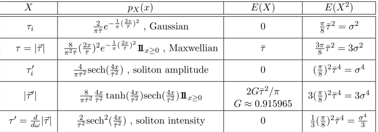
2.1 PMD-related probability density functions. . . 28

3.1 Peak-to-average ratio of different SCM schemes compared to NRZ. . . 46

3.2 Numerical values of SNRNRZ and SNRQAM−16 for different values of the BER. 47 3.3 16 QAM-16 SCM RF carrier frequency map. . . 48

3.4 System design “dimensions”. . . 68

5.1 Summary of system parameters. . . 136

5.2 System simulation platform and references to model descriptions. . . 139

5.3 System performance variations with fiber link length. . . 141

5.4 Summary of SNR requirements. . . 142

5.5 QAM transceiver test chip characteristics summary. . . 151

D.1 Values of the coefficients A and B in Eq. D.1 for a baseline BER of 10−9_{. . 188}

E.1 Vecteur PMD: densit´es de probabilit´e. . . 247

E.2 R´esum´e des param`etres de modulation choisis. . . 249 E.3 R´esum´e des caract´eristiques de la puce de modulation/d´emodulation QAM. 277

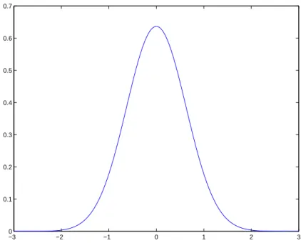
1.1 Simple optical link. . . 1 1.2 Integrated transponder module . . . 3 2.1 Loss and dispersion parameter of a standard single mode fiber. . . 8 2.2 Physical reference frame. . . 10 2.3 Polarization ellipse. . . 12 2.4 Poincar´e sphere. . . 16 2.5 Jones and polarization-ellipse Poncar´e sphere parameters. . . 17 2.6 Fiber transmission matrix. . . 23 2.7 Output SOP frequency dependence. . . 24 2.8 Principal States of Polarization. . . 27 2.9 Gaussian distribution for each component of the PMD vector ~τ. . . . 29 2.10 Maxwellian distribution for the DGD |~τ| . . . 29 2.11 Soliton-amplitude distribution for each component of ~τ0 _{. . . . 30}

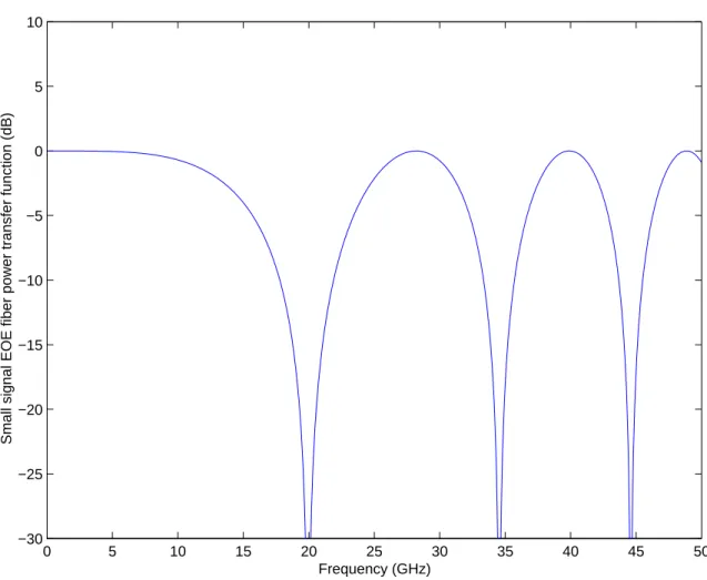
2.12 Illustration of higher-order PMD effects in fast-PSP pulse launch condition. 35 2.13 OOK NRZ signal with high level of PMD (all power in fast PSP). . . 37 2.14 OOK NRZ signal with high level of PMD (equal power in fast/slow PSP). . 38 3.1 Comparison of the power spectra of NRZ and QAM-16 over 16 carriers . . . 43 3.2 Subcarrier multiplexed system with receiver baudrate baseband DSP. . . 50 3.3 Inter-channel and image bands interference canceller. . . 56 3.4 Time-frequency equalization and cross-talk cancellation of channel k. . . . . 59 3.5 LMS adaptive filtering block diagram. . . 61 3.6 Block diagram of the adaptive time-frequency equalization DSP. . . 63 3.7 Enhanced time-frequency equalizer performance with 6-bit A/D resolution. 64 3.8 Enhanced time-frequency equalizer performance with 10-bit A/D resolution. 65

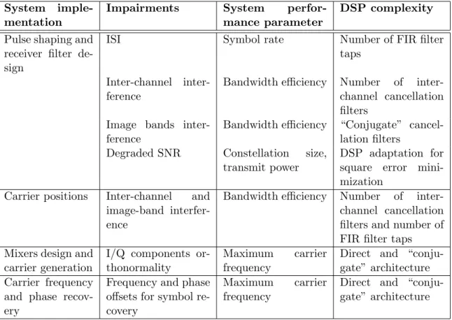
4.1 Optoelectronic transmission chain overview. . . 70 4.2 Electro-optical conversion. . . 71 4.3 Laser diode direct modulation. . . 71 4.4 IM/DD optical transmission scheme. . . 73 4.5 System representation of an intensity modulating source with chirp. . . 74 4.6 Definition of the input signal m. . . . 75 4.7 Definition of the output signal m_out. . . 75 4.8 EOE power transfer function: 10 km of fiber (1550 nm), unchirped source. . 79 4.9 EOE power transfer function: 10 km of fiber (1550 nm), source with negative

chirp. . . 81 4.10 EOE power transfer function: 10 km of fiber (1550 nm), semiconductor laser. 83 4.11 EOE response phase variations for 10 km of SMF at 1550 nm (DML case). . 84 4.12 EOE response group delay variations for 10 km of fiber at 1550 nm (DML case). 85 4.13 SSB filtering: phase variations at 1550 nm. . . 87 4.14 Concatenation of laser and 10 km of fiber EOE response. . . 89 4.15 Concatenation of laser and 40 km of fiber EOE response. . . 89 4.16 Laser clipping. . . 92 4.17 Signal and noise model at the optical receiver. . . 96 4.18 Linearized laser electro-optical frequency response amplitude. . . 106 4.19 Laser damping time Γ−1 vs. bias current. . . 108 4.20 Laser oscillation and resonance frequencies vs. bias current. . . 108 4.21 Laser relaxation oscillations . . . 109 4.22 Laser chirp when excited by a current step function. . . 109 4.23 Laser noisy behavior. . . 110 4.24 RIN power spectrum: theory vs. simulation. . . 110 4.25 RIN power spectrum: theory vs. measurements. . . 111 4.26 Intermodulation distortion of order 2. . . 112 4.27 Intermodulation distortion of order 3. . . 112 4.28 Setup for the measurement of intermodulation distortions. . . 114 4.29 Two-tone test result: example. . . 115 4.30 IIP2 at 50 mA above threshold. . . 115

4.33 IIP2 at 80 mA above threshold. . . 117 4.34 IIP2 at 90 mA above threshold. . . 117 4.35 IIP3 at 20 mA above threshold around f6. . . 118

4.36 IIP3 at 20 mA above threshold around f₉. . . 119 4.37 IMD3 around 14 GHz at 30 mA and 50 mA above threshold. . . 120 4.38 Simplified channel model. . . 123 4.39 RIN at laser resonance vs. bias current. . . 124 4.40 Laser natural bandwidth. . . 125 4.41 Laser diode capacity vs. bias current. . . 126 4.42 Capacity vs. fiber length. . . 127 4.43 Probability of no clipping impulse vs. bias current. . . 128 4.44 Laser capacity vs. OMI with RIN and clipping noise. . . 129 4.45 Signal-to-RIN ratio distribution: flat input signal power spectral density. . . 130 4.46 Capacity-optimal “Water-filling” input signal power spectral density. . . 132 4.47 Capacity-optimal signal-to-RIN ratio distribution. . . 133 5.1 SNR variations with bias current. . . 138 5.2 SNR variations with total OMI. . . 138 5.3 Test chip block diagram. . . 144 5.4 Test chip die photo. . . 145 5.5 Test chip measurement setups. . . 146 5.6 Transmit electro-optical and receive opto-electrical interfaces. . . 147 5.7 Test chip transmitter electrical output power spectrum. . . 149 5.8 Measured QAM-16 constellations. . . 150 5.9 Bandwidth efficient modulation optical transponder concept. . . 152 D.1 Dispersion induced pulse spreading. . . 185 D.2 Receive path with analog FIR filter. . . 191 D.3 Analog FIR FFE micrograph. . . 192 D.4 Equalization of 10 Gb/s NRZ signal impaired by PMD. . . 193 D.5 Compensator based on PSP alignment. . . 196 D.6 First order compensator. . . 197

D.9 Higher order compensator. . . 200 D.10 Block diagram of the experimental setup. . . 202 D.11 DOP calibration. . . 205 D.12 Spectral probe calibration. . . 207 D.13 Scan of the polarization controller. . . 209 D.14 QHQ polarization controller. . . 212 D.15 Convergence of the feedback loop. . . 215 D.16 Detailed block diagram of the experimental setup. . . 216 D.17 Typical compensator performance. . . 218 D.18 DOP scans. . . 220 D.19 Comparison of PC parameterization. . . 221 D.20 3-parameter compensator performance for 25 ps DGD. . . 223 D.21 3-parameter compensator performance for 50 ps DGD. . . 224 D.22 5-parameter compensator performance for 50 ps DGD. . . 225 D.23 Contribution of 1st_{-order PMD to the system performance degradation. . . 230}

D.24 Contribution of 2nd_{-order PMD to the system performance degradation. . . 231}

D.25 System performance measure. . . 232 D.26 Degree of polarization for different PC control parameter values. . . 233 D.27 Probed spectrum component for different PC control parameter values. . . 235 D.28 Optimal points comparison. . . 236 D.29 Probed spectrum component for different PC control parameter values. . . 238 D.30 Eye diagrams for maximized error signal. . . 240 E.1 Connection optique simple. . . 241 E.2 Matrice de transmission. . . 244 E.3 D´ependence en fr´equence du SOP en sortie. . . 245 E.4 Etats principaux de polarisation. . . 246 E.5 Densit´e spectrale de puissance de NRZ et QAM-16 sur 16 porteuses. . . 250 E.6 Syst`eme de communication `a sous-porteuses multiplex´ees. . . 251 E.7 Egalisation temps-fr´equence et suppression d’interf´erence dans le canal k. . 254 E.8 Bloc DSP pour l’´egalisation et la suppression d’interf´erences. . . 255

E.11 Chaˆıne de transmission opto´electronique: vue d’ensemble. . . 259 E.12 M´ethode de transmission IM/DD. . . 260 E.13 R´eponse lin´eaire de la chaˆne laser modul´e + 10 km de fibre. . . 261 E.14 Pincement laser. . . 263 E.15 Mod`ele de signal et bruit au niveau du r´ecepteur optique. . . 264 E.16 Amplitude de la r´eponse en fr´equence ´electro-optique lin´earis´ee du laser. . . 266 E.17 Densit´e spectrale de puissance de RIN: th´eorie et simulation. . . 267 E.18 Densit´e spectrale de puissance de RIN: th´eorie et mesures. . . 267 E.19 Montage pour la mesure des distorsions d’intermodulation. . . 268 E.20 IIP2 `a 50 mA au-dessus du seuil. . . 268 E.21 Mod´ele de canal simplifi´e. . . 269 E.22 Capacit´e en fonction de la longueur de fibre. . . 272 E.23 Capacit´e du laser en fonction de l’indice de modulation µ. . . 273 E.24 Variations du rapport signal sur bruit avec le courant d’op´eration laser. . . 275 E.25 Variations du rapport signal sur bruit en fonction de l’indice de modulation. 275 E.26 Sch´ema de la puce test. . . 277 E.27 Microphotographie de la puce test. . . 278 E.28 Constellation QAM-16 mesur´ee. . . 279

Introduction

1.1

Motivation for the study

Wireless and copper wireline communications have already greatly benefited from advances in digital signal processing (DSP). However optical communication is still widely based on simple on-off keying and the implementation of DSP techniques is very challenging at transmission rates in excess of 10 Gb/s. Higher speed such as 40 Gb/s require exotic and expensive optics and integrated circuit (IC) technologies. The research described in this dissertation is concerned with the use of modulation and DSP techniques in order to reduce the cost of optical transceivers and transponders with increased transmission capacity.

TOSA

ROSA

IC

IC

Fiber

Figure 1.1: Simple optical link. IC: integrated circuits; TOSA: transmit optical sub-assembly; ROSA: receive optical sub-assembly.

A functional block diagram of the type of optical communication links this dissertation focuses on is represented in Fig. 1.1. The fiber link stretches over a few tens of kilometers

and uses a unique wavelength for the purpose of short-reach high speed communications at 40 Gb/s and beyond. This excludes from the realm of this work long-haul applications and metropolitan wavelength-division multiplexing (WDM). Short distances spare the necessity of optical amplifiers. The fiber strand considered is made of standard single-mode fiber. It has a widespread installed base and is believed to be more amenable than multi-mode fiber to transmission speed scaling beyond already achievable rates of 10 Gb/s.

In this context, system cost is dominated by the transponder module terminating the link (excluding fiber material and installation cost which is shared by any system). A typ-ical structure for such a module is displayed in Fig. 1.2. Small form factor modules gather optical components and integrated circuits mounted on a printed circuit board within a single package providing standard electrical and optical input/output interfaces. Module cost is dominated by the cost of optical components. In essence, component bandwidth is the main cost driver: high bandwidth requirements demand exotic technologies, reduce production yield and call for enhanced packaging. Module power consumption is dominated by integrated circuits which pose a range of module design challenges in order to manage thermal dissipation. For speeds reaching tens of gigabit per second, the need for exotic integrated circuit technologies contributes both to cost (the material cost of a III/V com-pound wafer is more than ten times that of Si CMOS) and power consumption. CMOS technology has a significantly lower production cost than other technologies such as GaAs and InP when high production volumes are involved. Under this condition, mask cost, a fixed cost which is higher in the case of CMOS, is dominated by material and processing cost which is smaller for CMOS. Its cost advantage is even greater when the number of functions included on a single die increases, particularly for digital functions where high gate densities can be achieved.

1.2

Research context

This research work originates from an internship I performed from April to October 2000 within the High Speed Communications VLSI Research Department of Lucent Technologies Bell Labs in Holmdel, New Jersey. I later joined this department when it was being spun-off as part of Circuits and Systems Research Laboratory within the Lucent Microelectronics Division becoming Agere Systems, a newly independent company. At the time of the spin-off and when this research work was initiated, both optoelectronics and integrated-circuit

Analog Front-end S ta n d a rd e le ct ri ca l in te rf a c e Laser driver Receiver optics Transmitter optics Digital circuitry

Figure 1.2: Integrated transponder module.

expertises were being leveraged to produce innovative opto-IC communication semiconduc-tor solutions. This explains the multidisciplinary character of this research work carried out in an industrial context under the supervision of Prof. Gallion at ENST and the indus-trial mentorship of Dr. Azadet at Agere Systems. It greatly benefited from the interaction with renowned experts in the fields of opto-electronics, integrated-circuits design, signal processing and communications.

1.3

Overview of the thesis

Models for the transmission of optical signals in standard single mode fibers are presented in Chapter 2. Fiber-guided light can be described by a finite number of degrees of freedom (intensity, phase, state of polarization) that can all in principal be used to convey informa-tion over great distances. Most systems use light power as the conveyor of informainforma-tion. In systems that employ multiple wavelengths over distances of several hundred of kilometers, such as in wide area networks (WAN) and transoceanic networks, launch power is high and models need to include the fiber material nonlinear response. Yet for shorter distance applications, such backplane, data center communications, local area networks (LAN) and metropolitan area networks (MAN), the optical launch power is more modest and nonlin-ear products do not accumulate significant power in short distances. In these cases fiber

response can be assumed to be linear. A simple input/output linear model can be derived under this assumption describing the transmission of optical waveforms impaired by fiber dispersion. Illustration of the predictions of the models and their numerical implementation are presented in the case of the simple and widely used on-off keying (OOK) format.

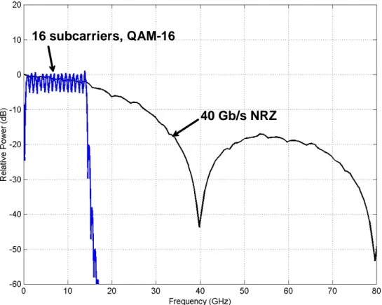
Getting away from OOK, chapter 3 describes advantages and drawbacks of sub-carrier multiplexing (SCM) with multilevel signaling as a bandwidth efficient modulation scheme. The main motivation for using such a modulation lies in the lower signaling rate per radio-frequency (RF) carrier channel allowing the complex processing of multilevel signals with standard CMOS technology at low power consumption levels. Advanced digital signal processing (DSP) that was previously only the prerogative of wireless systems becomes accessible to optical communications. This brings a multitude of benefits ranging from the ability to effectively implement the promised bandwidth efficiency to easing circuit design constraints.

The definition of an optical link employing SCM for the transmission of 40 Gb/s is introduced in Chapter 4. The selection of link components based on their cost and wide-spread availability through volume industrial production is outlined before diving into the details of their operation. Sub-carrier multiplexing is sensitive to transmission link non-linear impairments. All impairment contributions are evaluated using realistic component characteristics. These contribution estimates motivate the precise modelling of the directly modulated laser (DML) source. These models are supported by experimental validation. In addition, a simplified information channel model is defined taking into account trans-mitter and receiver noise as well as laser clipping distortion. It provides the basis for the evaluation of the channel capacity and the investigation of its dependence on key parame-ters such as the laser bias current, the optical modulation index and the fiber length. The computed capacity and associated spectral efficiency offer a theoretical reference point for the implementation of a communication system based on such a channel.

Chapter 5 brings together models and concepts introduced in previous sections for the specification of a transmission system based on an integrated CMOS transceiver. A com-plete simulation platform was implemented to establish the feasibility of such a system and to provide a set of specifications for system implementation. These specifications are used to design a single-channel QAM transceiver test chip in 0.14-µm CMOS technology. The test chip proves that design challenges already encountered in wireless applications at lower frequencies can be overcome at frequencies approaching 14 GHz. Measurement results

for a single-channel transmission link are presented. The link is composed of the CMOS transceiver test chip connected through appropriate amplification stages to an optical link comprised of a DML, 30 km of fiber and a p-i-n photoreceiver.

Chapter 6 draws the conclusions of this research work and makes suggestions for future investigations. In an effort to provide a steady and coherent flow of information more detailed calculations as well as related developments are gathered in appendices at the end of this dissertation.

Optical Fiber Modeling

This chapter provides a mathematical description of the input/output signal transmission behavior of single-mode optical fibers with an emphasis on dispersion due to the fiber birefringence. Fiber impairments are illustrated and discussed here in the context of on-off keying (OOK) optical transmission which is the most widely used optical modulation format.

Most complete and accurate fiber propagation models are based on partial differential equations describing the evolution of the optical field along the fiber length. Yet in a linear operation regime this description can be greatly simplified leading to a general form for the fiber ’black box’ model that depends on a few basic quantities characterizing the different effects on transmitted optical signals.

These characteristic quantities could very well be defined in a more general framework. But in the case of optical fibers, additional modelling assumptions can be applied that lead to characteristic properties (specific numerical values or statistical distributions). These characteristic properties can be used as a basis for determining the actual magnitude of fiber dispersive effects on the signal integrity and devising mitigation strategies.

The fiber ’black box’ model can be further simplified to provide efficient computational models for numerical simulation purposes.

2.1

Optical fibers

In an optical communication link an information-bearing electrical signal is converted into an optical signal that propagates through an optical fiber and is converted back into an

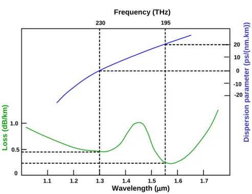
1.1 1.2 1.3 1.4 1.5 1.6 1.7 -20 20 10 0 -10 230 195 Frequency (THz) Wavelength (µµµµm) 0.5 1.0 0 L o s s ( d B /k m ) D is p e rs io n p a ra m e te r (p s /( n m .k m ))

Figure 2.1: Loss and dispersion parameter of a standard single mode fiber.

electrical signal. In the case of single-mode fibers the optical signal can undergo a number of distortions due to the fiber material properties (doped silica) and geometry. A broad description of those effects as well as historical notes and typical values for commercially available fibers can be found in [Ref99].

1. Linear distortions Attenuation

An optical signal gets attenuated as it propagates over a stretch of fiber. The attenuation curve of a typical silica-based fiber is shown in Fig. 2.1. Its shape exhibits three types of features related to different physical phenomena. Firstly it has an overall tendency to increase with decreasing (vacuum) wavelength below 1.3 µm due to Rayleigh scattering. Secondly it shows absorption peaks due to the hydroxyl ion (OH−_{) around 1.45 µm. And thirdly it has a tendency to}

increase above 1.6 µm due to bending-induced loss and silica absorption. Silica-based fiber has two low-loss windows, one around the wavelength 1.3 µm and one

around 1.55 µm, which are both used in optical communication. Common single-mode fibers have a loss of approximately 0.4 dB/km at 1.3 µm and 0.25 dB/km at 1.55 µm.

Chromatic dispersion

Due to material and geometrical properties of glass fiber different wavelengths travel at different speeds. If chromatic distortion is high, optical pulses tend to broaden as they go down the fiber link. In digital optical communication systems, this can lead to inter-symbol interference and system performance degradation. Polarization Mode Dispersion (PMD)

Despite its name the single-mode fiber generally allows for two polarization modes to propagate. These modes have different propagation properties when the fiber is not perfectly circularly symmetrical or is put under mechanical stress, their orientation is a priori unknown and can vary with time and wavelength. So light pulses generally incur broadening after transmission since they come out of the fiber as a superposition of two polarized pulses with different arrival times. 2. Nonlinear distortions

Stimulated scattering

This form of scattering occurs when an intense optical signal interacts with acoustic waves (Stimulated Brillouin Scattering) or with molecular modes of vibration (Stimulated Raman Scattering) within silica fiber.

Refractive index fluctuations

High optical power variations can locally modulate the material index. In turn, this index modulation alters the propagation of the optical signal itself (Self-Phase Modulation) or of other signals on other wavelength channels (Cross-(Self-Phase Modulation) in wavelength-division multiplex (WDM) systems. It can also result in the mixing of optical signals at two or three wavelengths (Four-Wave mixing) into one or more other wavelength channels.

The impact of these phenomena on the integrity of the signal of interest varies with operating parameters (wavelength, input power, fiber length, fiber manufacturing and envi-ronmental conditions, etc.). Differentiating different regimes of operation distinguishes the main contributors. It is of paramount importance in the derivation of an optical channel model that provides the best trade off between simplicity and accuracy.

In the following section we briefly review models for the description of the optical signal and its propagation in single-mode fibers.

2.2

Mathematical models

Light is the “messenger” that carries our signal through the fiber. Hence our description of the effects on the transmitted signal depends on our description of light. A “good” representation has to describe every phenomenon of interest and be simple. This is why the classical (i.e., non quantum-mechanical) theory of light will form the general framework for this representation here. If needed, quantum effects will be added by assuming that light is composed of photons following specific statistical distributions in space and time.

2.2.1 Guided light beam representation

x

y

z L

Figure 2.2: Physical reference frame.

Degrees of freedom Our main premise at this point is that the guided light wave can be represented by a two-dimensional complex vector at each point of space and time in a reference frame such as the one represented in Fig. 2.2

A(z, t)eiω0t₌

Ã

Ax(z, t)

A_y(z, t) !

eiω0t_,

where ω₀ is the angular optical frequency of the modulated optical carrier and A(z, t) the slowly varying part of the optical signal. This field is a solution of a wave equation stemming from the Maxwell equations in a dielectric medium, the electromagnetic response of that medium and its geometrical properties. It is useful to represent the propagation equations and their solutions in the Fourier domain

˜

A(z, ω) =

Z

A(z, t)e−iωtdt,

where ω is the angular frequency relative to the optical carrier angular frequency ω0.

The Fourier representation allows an account of the number of degrees of freedom: the field can be viewed as a collection of complex functions in space indexed by a particular frequency. Each of these functions is completely determined by its value at one particular point (for instance z = 0, the input of the fiber). For each frequency we then have four degrees of freedom since each component can be specified by its real and imaginary parts or amplitude and phase (which depend on z and ω). The slowly varying part of the optical field can be written

˜

A(z, ω) = a(z, ω)|si_(z,ω) (2.1) where |si =

Ã

s1

s₂

!

is a complex vector such that ksk2 = |s1|2+ |s2|2 = 1

and a(z, ω) is the complex amplitude and |si_(z,ω) the State of Polarization (SOP) of the field at a certain frequency and at a certain point in space. The Dirac notation for two-dimensional complex vectors and their duals is used: |si =

à s₁ s2 ! , hs| = (s∗ 1, s∗2).

We can make a few comments at this point. The decomposition (2.1) is not unique since another valid one is ˜A = a0_|s0_{i with a}0 _{= e}iθ_{a and |s}0_{i = e}−iθ_{|si , θ being an arbitrary}

function of z and ω, and this way we have accounted for every decomposition of that kind. The state of polarization of light refers to this family of unit complex vectors differing from each other by a multiplicative unit-modulus complex number. It can also be noted that complex amplitude and SOP bear different kinds of information: the first one gives the power and common phase of the field whereas the second one describes the relative power and relative phase of its two components once a physical reference frame has been chosen.

State of polarization representation In the following section we consider one particular frequency component ω of the field at one particular point in space z without necessarily referring to those quantities. We describe three representations for the SOP: the polarization ellipse representation, the Jones representation and the Poincar´e sphere representation.

Polarization ellipse We imagine here that for an arbitrarily specified relative angular frequency, ω, the signal is composed of the single frequency component ˜A at ω + ω0. A

complete expression of the field vector in the time domain can be written

˜ Aei(ω+ω0)t₌ Ã | ˜Ax|eiφx, | ˜Ay|eiφy ! ei(ω+ω0)t_,

which gives, if we project it on the subspace of real vectors

Re( ˜Aei(ω+ω0)t_{) =} Ã | ˜Ax| cos((ω + ω0)t + φx) | ˜Ay| cos((ω + ω0)t + φy) ! .

If we graphically represent the time-parameterized curve thus generated in the x-y reference frame, we get an ellipse. If we normalize this vector so that |Ax|2+ |Ay|2 = 1 and change

the time reference so that φx = 0, we end up with a family of ellipses that graphically

represent the states of polarization of the field vector. That family can be indexed by two independent real numbers α ∈ [0, π[ and γ ∈ [−π/4, +π/4] as shown in Fig. 2.3.

x y

α

γ

Figure 2.3: Polarization ellipse.

The names given to SOP’s comes from this representation. If the ellipse is “degenerate” (γ = 0), the SOP is said to be linear. If, added to this, its axis is aligned with the x-axis (α = 0), the state of polarization is said to be horizontal (H). If it is aligned with the y-axis (α = π/2), it is said to be vertical (V). If the ellipse is a circle, the SOP can be a right

(lcp) if it rotates counter-clockwise (γ = −π/4)1_.

Jones representation We have seen that the field vector can be written ˜ A = Ã | ˜A_x|eiφx | ˜Ay|eiφy !

= a|si with ksk2= hs|si = 1,

which is equivalent to the relations            a = q | ˜Ax|2+ | ˜Ay|2 eiφ |si = Ã cos(θ/2)ei(φx−φ) sin(θ/2)ei(φy−φ) ! with      cos(θ/2) = _√ | ˜Ax| | ˜Ax|2+| ˜Ay|2 sin(θ/2) = _√ | ˜Ay| | ˜Ax|2+| ˜Ay|2

where the phase φ is either arbitrarily chosen, or constrained by a propagation equation or any other relationship.

If we talk about the SOP of the field without relating the notion to a specific situation, this phase is arbitrary. Changing φ changes the Jones vector |si but does not change the represented SOP. Thus, a more suitable way of representing SOP’s is to use equivalence classes. On the set of Jones vectors J = {|si ∈ C2_{; ksk}2 _{= 1} we define the equivalence}

relationship |s1i ∼ |s2i ⇐⇒ ∃φ ∈ R, |s1i = eiφ|s2i. The SOP of light can be defined as the

corresponding equivalence class. Each class can be designated by one of its elements. We can add a constraint to the choice of the representative so that one and only one representative can be picked in each class (except possibly for a finite number of degenerate cases). This allows the representation SOP’s with Jones vectors in an unambiguous way. For instance we can add the constraint that, assuming a particular orthonormal basis has been chosen in C2 _{(which can be related to a physical reference frame), the representative of each class}

is the element with a first component that is real. The corresponding parameterization of the SOP’s is _Ã

cos(θ/2) sin(θ/2)ei∆

!

with θ ∈ [0, π] and ∆ ∈ [0, 2π[. (2.2) A parameterization that “splits” the relative phase between the two components is often

1_{The “right” and “left” denomination is arbitrary and has only a historical explanation. The contrary}

used _Ã

cos(θ/2)e−i∆/2

sin(θ/2)e+i∆/2

!

with θ ∈ [0, π] and ∆ ∈ [0, 2π[. (2.3) If the constraint does not come from another physical equation, any choice is good as long as every subsequent statement is consistent with it. The parameters θ and ∆ can be related to the polarization ellipse parameters. As a matter of fact it can be shown that each SOP can be represented by the pair (θ, ∆) or the pair (α, γ) and

à cos(θ/2) sin(θ/2)ei∆ ! ∼ à cos(θ/2)e−i∆/2 sin(θ/2)e+i∆/2 ! ∼ Ã

cos(α) cos(γ) − i sin(α) sin(γ) sin(α) cos(γ) + i cos(α) sin(γ)

!

. (2.4)

Poincar´e sphere representation In the previous section we have seen that the states of polarization could be mathematically represented with equivalence classes over the set of Jones vectors. Though Jones vectors can be expressed in a specific basis that corresponds to a given physical reference frame, as mathematical objects they do not refer to any particular one. Consequently the same holds for the SOP’s themselves. This very independence to any basis will lead us to the natural structure of the set of SOP’s and a very powerful way to represent their evolution when passed through an optical system. This representation is not introduced here from more basic assumptions. Its structure and properties will simply be described.

The set of SOP’s can be mapped onto a subset of the real space R3_{. The dimensionality of}

this subset can already be derived from the fact that the set of SOP’s is parameterized using two independent real parameters. More precisely let σ1 =

à 1 0 0 −1 ! , σ2 = à 0 1 1 0 ! and σ3 = à 0 −i i 0 !

be the Pauli matrices2 _{which form an R-basis of the space of the 2 × 2}

traceless Hermitian matrices. Let ~σ be the following column

~σ =     σ1 σ₂ σ3     .

A map can be defined by picking for each SOP one of its Jones representatives and by

2_{In quantum mechanical problems, they are traditionally referred to as σ}

associating the following vector of R3 ~ S = hs|~σ|si =     hs|σ1|si hs|σ2|si hs|σ3|si     =     |s1|2− |s2|2 s∗₁s2+ s∗2s1 −i(s∗ 1s2− s∗2s1)     . (2.5)

The vector ~S does not depend on the representative |si that has been chosen but only on

its equivalence class that is to say the SOP. This map is consequently well defined. It can be shown that this map is one-to-one from the set of SOP’s to the unit radius sphere of R3. In the present context this sphere is called the Poincar´e sphere.

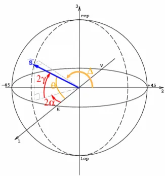
Through the map defined by (2.5) each parameterization of Jones vectors implies one for the sphere. The parameterizations (2.2) and (2.3) lead to the following for the Poincar´e sphere ~ S(θ, ∆) =     cos(θ) sin(θ) cos(∆) sin(θ) sin(∆)     θ ∈ [0, π], ∆ ∈ [0, 2π[. (2.6) We recognize here a standard spherical coordinate system relative to the first canonical basis vector (direction 1 in Fig. 2.4). The polarization ellipse parameterization expressed in (2.4) leads to a different description of the sphere

~ S(α, γ) =     cos(2α) cos(2γ) sin(2α) cos(2γ) sin(2γ)     α ∈ [0, π[, γ ∈ [−π/4, +π/4]. (2.7) We recognize here an “azimuth-elevation” or “longitude-latitude” coordinate system relative to the third canonical basis vector (direction 3 in Fig. 2.4). 2α stands for the longitude and 2γ for the latitude. Fig. 2.4 shows correspondence between points on the sphere and polarization ellipses.

Fig. 2.5 shows the geometrical correspondence between (θ, ∆) and polarization-ellipse parameters (α, γ). It is important to notice that axes 1, 2 and 3 are associated with a given physical reference frame x-y although the three-dimensional real space in which the sphere is embedded is not directly related to the physical space. Circles of constant γ gather the SOP’s with same ellipticity but varying orientation of the ellipse longest principal axis. The semicircles of constant α gather the SOP’s with same principal axis orientation but with

rcp +45 −45 H V 1 2 3

2α

2γ

Figure 2.4: Poincar´e sphere.

different ellipticities. The “northern hemisphere” is composed of the right SOP’s and the “southern hemisphere” the left SOP’s. The circles of constant θ gather the SOP’s with the same power distribution among their two components but with different relative phases. The semicircles of constant ∆ are composed of the SOP’s with the same relative phase but with different power distribution among their x-y components.

2.2.2 Guided light beam propagation in single-mode fibers

There is an abundant literature deriving models for the propagation of the optical field along a single-mode fiber starting from the basic laws of electromagnetism and the response of the fiber material to the electromagnetic excitation (see for instance [Agr95b] and [Fra91]). They vary in the set of effects they intend to capture but they all result in the definition of a partial differential equation relating the variations of the optical field over the fiber length to the local value of the field and its time derivatives.

Nonlinear Shr¨odinger equation Given the geometrical structure of the fiber (cylin-drical core and cladding having different dielectric properties), it can be shown (see [Agr95b]

Figure 2.5: Relation between the Jones and polarization-ellipse coordinate systems on the Poincar´e sphere.

for instance) that if the diameter of the core is small enough (less than 10 µm for the wave-lengths used in optical communications) only one spatial mode can propagate at the angular optical wavelength, ω0, having wavelength in vacuum λ0 = 2πc_ω0 . The electrical field takes

the following variable-separated form

E(~r, t) = Re

³

F (x, y)B(z, t)eiβ0z_e−iω0t

´

,

where F (x, y) describes the spatial distribution of the mode power in the x-y plane and

B(z, t) the z and temporal evolution of the slowly varying part of the field. F can be

satisfyingly approximated by a Gaussian distribution. It is customary and convenient to normalize F such that RR|F (x, y)|2dxdy = 1. Then |B(z0, t0)|2 gives the optical power

crossing the fiber section z = z0 at the time t = t0.

Once all this has been stated and kept in mind, it appears that B itself bears all the information about the optical field in the fiber. If it were a two-dimensional quantity it could be identified with the description of the field given in section (2.2.1). In fact, this can be done as will be made clearer in the next section. As shown in [Agr95b] and [Fra91] B

is a solution of the propagation equation called the Nonlinear Schr¨odinger (NLS) equation expressed here in the time domain

∂B ∂z + β1 ∂B ∂t + i 2β2 ∂2_B ∂t2 + α 2B = iγ|B| 2_B,

where α is the attenuation coefficient of the fiber and γ is the nonlinearity coefficient given by

γ = n2ω0 cAeff,

where A_eff =³ RR|F (x, y)|2_dxdy´2_/RR_{|F (x, y)|}4_{dxdy is the effective core area and n}

2 is the

nonlinear refractive index. In optical fibers a typical value for n2 is 3 · 10−20m2W−1 for

wavelengths around 1.5 µm. Typically A_eff ≈ 50−80 µm2 _{at λ}

0 ≈ 1.5 µm. The coefficients

β1 and β2, and their association with time derivatives of the corresponding order, stem from

the truncation of the Taylor expansion of the propagation coefficient β(ω) ≈ β0 + β1ω + 1

2β2ω2 in the frequency domain in the vicinity of the optical carrier frequency. Those latter

coefficients are related to other customary quantities: the group velocity vg = 1/β1 and the

chromatic dispersion coefficient D = dβ1

dλ = −2πcλ2

0 β2. As a matter of fact β1 is the group

delay experienced by a transmitted light pulse per unit length of fiber and the chromatic dispersion coefficient D quantifies the variations of this group delay per unit length with wavelength. β2 = dβ_dω1 is another measure of chromatic dispersion and is called the group

velocity dispersion (GVD) parameter. Typically D ≈ 17 ps/(nm · km) at λ0 ≈ 1.5 µm for a

single-mode fiber (SMF) which means that a change in wavelength of 1 nm will change the group delay by 17 ps in a 1 km-long piece of fiber.

A better form for the NLS equation is obtained through the change of variable T =

t − β1z = t − z/vg that describes the field in a reference frame moving along the fiber at

the same speed vg as a pulse

∂B ∂z + i 2β2 ∂2_B ∂T2 + α 2B = iγ|B| 2_{B, (2.8)}

Numerical solutions for this nonlinear partial differential equation can be computed using the split-step Fourier method presented in [Agr95b].

Coupled non-linear Shr¨odinger equation If we now take into account fiber bire-fringence, the NLS equation can be modified in order to model this effect. The model

introduces the birefringence vector ~β, a quantity that is defined along the fiber length and

describes the action on the polarization of light of infinitesimal pieces of fiber at each point of the fiber span as explained in Appendix A. To include the effects of fiber distributed bire-fringence [Men89] makes the assumption that the birebire-fringence vector variations takes the form ~β(z, ω) = (2b + 2b0_{ω)~n(z) where 2b is the birefringence strength at ω}

0, b0 is the

deriv-ative of b with respect to ω at ω0 and ~n is a unit length vector following a diffusion process

(random walk) parameterized by z. With these assumptions the field vector B = Ã

Bx

B_y

!

evolution is governed by the Coupled Nonlinear Schr¨odinger (CNLS) equation

i∂B ∂z + b ¡ ~n · ~σ¢B + ib0¡~n · ~σ¢ ∂B ∂T | {z } birefringence −1 2β2 ∂2_B ∂T2 | {z } chromatic dispersion +iα 2B | {z } loss + γ ³ |B|2B −1 3 ¡ B†σ3B ¢ σ3B ´ | {z } monlinear effects = 0, where B†₌³ _B∗ x,By∗ ´

and as previously defined T = t − β1z.

We note the importance of the second birefringence term involving the quantity b0 _in

accounting for polarization-dependent group delays as the presence of the ∂/∂T operator suggests. If the birefringence strength is not frequency dependent there is no polarization-related dispersion. In this case the action of the fiber is a simple state of polarization rotation and it does not have an impact on the transmission of optical signals encoded in the light beam complex amplitude.

Numerical solutions for this stochastic differential equation can be computed using the coarse-step method. This is basically the same as the split-step Fourier method for the NLS except for a pseudo-random scrambling of the SOP of the data after each step thus emulating the effect of an randomly oriented infinitesimal birefringent element.

Fiber operation regimes If we want to study the evolution of an input pulse of width T0 and peak power P0, the NLS equation can be rewritten in a way that highlights

every important phenomenon and naturally associates physical lengths to them. Let τ =

T /T₀ be the new time variable and B(z, T ) =√P₀e−α₂z_{u(z, τ ). u is now a quantity with no}

dimension and the NLS equation (2.8) is equivalent to

i∂u ∂z = sgn(β₂) 2LD ∂2_u ∂τ2 − e−αz LNL|u| 2_,

where sgn(β2) is the sign of the GVD parameter β2, LD = T02/|β2| is the dispersion length

and LN L= (γP0)−1is the nonlinearity length. LD and LN Lare the length scales over which

the dispersive and nonlinear effects respectively become significant in the propagation of optical signals. If one of those two lengths is greater than the fiber strand length L the corresponding phenomenon does not accumulate significantly to play an important role on the evolution of the pulse.

A length scale LP M D can also be associated with polarization-mode dispersion (PMD).

Due to the stochastic nature of PMD L_{P M D} has to be inferred by other means than nor-malization of the CNLS. Since the main purpose of this section is the evaluation of the importance of nonlinear optical effects, we refer to Sec. 2.3.4 for a discussion on the length scale associated with polarization-mode dispersion. In cases where a linear approxima-tion cannot be made [Men89], [WM96], [MMW97], [WMZ97] and [MMW97] define other length scales distinguishing a variety of operation regimes determined by the interaction of polarization-related effects and nonlinear effects.

If we consider an on-off keying (OOK) digital transmission at the wavelength λ0 ≈

1.55 µm and at a bit rate D_bthrough a standard SMF (D = 17 ps/(nm · km), A_eff ≈ 50 µm2_,

γ ≈ 2.10−3_m−1_{· W}−1_{), we then have} L_D ≈ 5000 (Db[Gb/s])2 km, L_{N L} ≈ 500 Po[mW] km.

In the case of a broadband point-to-point connection suitable for a LAN or a MAN we typically have fiber spans with length L < 80 km. If we use Po ≈ 4 mW which is typical

for such configurations we have L_{N L}≈ 125 km. In this case we can assume that non-linear

phenomena do not play an important role in the propagation of light pulses. In comparison a linear phenomenon such as chromatic dispersion cannot be neglected for communications at speeds in excess of 10 Gb/s since we have in this case LD less than 50 km. We will

2.3

Fiber models in the linear regime

2.3.1 Introduction

In this section we introduce the optical transmission matrix describing a fiber piece linear in-put/ouput behavior using the linearized version of the field propagation equation presented in the previous section. We emphasize its structure, thus highlighting some assumptions that form the basis for the derivation of the original propagation equation as well.

The parameter dependence of the transmission matrix allows us to define important quantities used for describing polarization-related dispersive effects on the transmission of optical signals: the PMD vector and the differential group delay (DGD).

Whereas the general form of the transmission matrix could be applied to a variety of optical systems the actual parameter dependence of the transmission matrix can be further modelled in the case of optical fibers. Successful stochastic and distributed models have been proposed, the theoretical predictions of which are validated by experimental results. We report the main results regarding the statistics of PMD highlighting basic parameters characterizing the strength of the phenomenon and commonly used by fiber and fiber cable manufacturers.

That knowledge does not allow the derivation of a simple form for the transmission matrix though and further approximations have to be made to arrive at simple expressions suitable for modelling the transmission of narrowband optical signals used for the trans-mission of digital data using an on-off keying modulation format. These simple expressions when applied in their domain of validity are very useful for the implementation of efficient numerical simulations allowing the effective exploration of fiber dispersive effects on optical signals with the design of optical communication systems or subsystems in mind.

2.3.2 Fiber transmission matrix

As a preliminary comment, note the use of different names (A in Sec. 2.2.1 and B in Sec. 2.2.2) to represent the optical field. This provides the opportunity to clarify differences in notations one can find in the literature depending on whether the subject matter is optical fiber propagation equations or input/output relationship. Up to this point the propagation equations were not formulated using the optical field A since it can lead to confusion when comparing to expressions in the literature. One convention is widely used for representing

the electrical field when dealing with field propagation equations in optical fibers

E(~r, t) = Re

³

F (x, y)B(z, t)eiβ0z_e−iω0t

´

,

where we note that the carrier phase term is −ω₀t at z = 0. The definition of the Fourier

transform ˆB of B is chosen accordingly and we have ˆB(z, ω) =R B(z, t)e+iωt_{dt and reversely}

B(z, t) = _2π1 R B(z, w)eˆ −iωt_{dω. Another convention is used for representing the electrical}

field when using a system approach to optical fiber effects

E(~r, t) = Re

³

G(x, y)A(z, t)e−iβ0z_e+iω0t

´

,

where the carrier phase term is +ω0t at z = 0 and the Fourier transform ˜A of A is defined

as ˜A(z, ω) = R A(z, t)e−iωtdt and A(z, t) = _2π1 RA(z, ω)e˜ +iωtdω. In the remainder of this

document the latter convention will be used. To reconciliate the two representations we note that they represent the same physical electrical field and that we can switch from one to the other by complex conjugation: A(z, t) = B∗_{(z, t) in the time domain and ˜A(z, ω) = ˆB}∗_{(z, ω)}

in the frequency domain.

The linear propagation equation including chromatic and birefringence effects can be written the following way using the optical field A

∂ ˜A ∂z + i 1 2β.~σ ˜~ A + i ¯β ˜A + α 2A = 0,˜

where the propagation coefficient ¯β(ω) = β(ω) − β0 can be expanded around the center

frequency, ¯β(ω) ≈ β1ω + 1₂β2ω2 and ~β(z, ω) is the birefringence vector.

We can condense this equation by writing ˜C = ˜Aeα2zei ¯β(ω)z,

∂ ˜C

∂z + i~β.~σ ˜C = 0.

Since we have a linear ordinary differential equation in z for ˜C with initial condition

˜

A(0, ω) = ˜Ain(ω) for each ω we can write

˜

C(z, ω) = U (z, ω) ˜C(0, ω),

Figure 2.6: Fiber transmission matrix modelling the fiber input/output linear behavior.

matrices and satisfies ₍

U (0, ω) = I2

∂U

∂z + i12β.~σU = 0~

(2.9)

where I2 is the 2x2 identity matrix. It directly stems from the fact that ~β.~σ takes its values

in the space of the 2x2 traceless Hermitian matrices that, for all z and ω, U (z, ω) is in

SU (2) as explained in Appendix A. The optical field A at any point in the fiber can be

expressed as a function of the input ˜

A(z, ω) = e−α2ze−i ¯β(ω)zU (z, ω) ˜A_in(ω).

We consequently have a general expression for the transmission matrix T that relates the output of the fiber ˜Aout(ω) = ˜A(L, ω) to its input ˜Ain(ω) = ˜A(0, ω):

T (ω) = e−α2Le−i ¯β(ω)LU (L, ω), (2.10)

where L is the fiber length. From a system point of view the fiber is modelled as a black box with an optical input, an optical output and a linear relationship between those two quantities ˜Aout(ω) = T (ω) ˜Ain(ω) as illustrated in Fig. 2.6.

The transmission matrix T is the product of two terms:

T (ω) = e−(α2+i ¯β(ω))LM (ω), (2.11)

where the first term, the common propagation term, is a complex function of ω and the second term M (ω) = U (L, ω), the birefringence or Jones matrix, is a function of ω that takes its values in SU (2). The transmission matrix T acts separately on the common complex amplitude and the SOP of the optical field. The common propagation term relates the

M(

ω

)

R(

ω

)

|s

〉

|s

(

ω

)

〉

S

S

(

ω

)

Figure 2.7: Illustration of the frequency dependence of the output SOP due to the frequency dependence of the input/output linear relationship.

input and output complex amplitudes and accounts for common group delay, chromatic dispersion and loss. The birefringence matrix M establishes the relationship between the input and the output SOP and accounts for a polarization-dependent group delay and chromatic dispersion. This can be further stated by writing ˜A = a|si as in Eq. 2.1 and

expressing the input-output relationship for complex amplitude and SOP

aout= e−(

α

2+i ¯β(ω))La_in and |s_outi = M |s_ini.

We have seen that the SOP can either be represented by a Jones vector or by a vector on the Poincar´e sphere embedded in a three-dimensional real space called the Stokes space. As explained in Appendix A, the input-output SOP relationship can also be expressed in Stokes space

~

Sout(ω) = R(ω)~Sin,

where R(ω) is the rotation corresponding to the Jones matrix M (ω). It will be assumed in every case that the input optical field is completely polarized as can be produced by a laser source. The frequency dependence of M leads to a frequency dependent output SOP and depolarization of the light beam.

As noted earlier the action of the transmission matrix does not mix all the degrees of freedom. This comes from the fact that the local birefringence vector has only real components. A complex valued birefringence vector would mean that there exist in the system distributed sources of loss or gain that are sensitive to the light beam SOP. In real optical systems we can actually find sources of polarization-dependent loss (PDL) but they usually do not come from the fiber itself. Furthermore, they are generally generated by elements at the end the link (polarization beam splitters, optical amplifiers,...). So they can