HAL Id: pastel-00004041
https://pastel.archives-ouvertes.fr/pastel-00004041
Submitted on 18 Jul 2008HAL is a multi-disciplinary open access archive for the deposit and dissemination of sci-entific research documents, whether they are pub-lished or not. The documents may come from teaching and research institutions in France or abroad, or from public or private research centers.
L’archive ouverte pluridisciplinaire HAL, est destinée au dépôt et à la diffusion de documents scientifiques de niveau recherche, publiés ou non, émanant des établissements d’enseignement et de recherche français ou étrangers, des laboratoires publics ou privés.
Variable Bandwidth Image Models for
Texture-Preserving Enhancement of Natural Images
Noura Azzabou
To cite this version:
Noura Azzabou. Variable Bandwidth Image Models for Texture-Preserving Enhancement of Natural Images. Mathematics [math]. Ecole des Ponts ParisTech, 2008. English. �pastel-00004041�
TH `ESE
pr´esent´ee pour l’obtention du titre de
DOCTEUR DE L’ ´ECOLE DES PONTS
Sp´ecialit´e : Math´ematiques, Informatique
par
Noura Azzabou
Variable Bandwidth Image Models for
Texture-Preserving Enhancement of Natural
Images
Soutenue le 31 Mars 2008 devant le jury compos´e de : Rapporteurs Rachid Deriche INRIA Sophia Antipolis
Nir Sochen Tel Aviv University
Alan Willsky Massachusetts Institute of Technology Examinateurs Jean Yves Audibert Ecole des Ponts
Jean Michel Morel ENS Cachan Directeurs de th`ese Fr´ed´eric Guichard DxOLabs
Nikos Paragios Ecole Centrale de Paris Membres invit´es Fr´ed´eric Cao DxOLabs
Abstract
This thesis is devoted to image enhancement and texture preservation issues. This task involves an image model that describes the characteristics of the recovered signal. Such a model is based on the definition of the pixels interaction that is often characterized by two aspects (i) the photometric similarity between pixels (ii) the spatial distance between them that can be compared to a given scale. The first part of the thesis, introduces novel non-parametric image models towards more appropriate and adaptive image description using variable bandwidth approximations driven from a soft classification in the image. The second part introduces alternative means to model obser-vations dependencies from geometric point of view. This is done through statistical modeling of co-occurrence between observations and the use of multiple hypotheses testing and particle filters. The last part is devoted to novel adaptive means for spatial bandwidth selection and more efficient tools to capture photometric relationships between observations. The thesis concludes with pro-viding other application fields of the last technique towards proving its flexibility toward various problem requirements.
R´esum´e
Cette th`ese s’int´eresse aux probl`emes de restauration d’images et de pr´eservation de textures. Cette tache n´ecessite un mod`ele image qui permet de caract´eriser le signal qu’on doit obtenir. Un tel model s’appuie sur la d´efinition de l’interaction entre les pixels et qui est caract´eris´e par deux aspects : (i) la similarit´e photom´etrique entre les pixels (ii) la distance spatiale entre les pixels qui peut ˆetre compar´ee `a une grandeur d’´echelle. La premi`ere partie de la th`ese introduit un nouveau mod`ele non param´etrique d’image. Ce mod`ele permet d’obtenir une description adaptative de l’image en utilisant des noyaux de taille variable obtenue `a partir d’une ´etape de classification effectu´ee au pr´ealable. La deuxi`eme partie introduit une autre approche pour d´ecrire la d´ependance entre pixels d’un point de vue g´eom´etrique. Ceci est effectu´e `a l’aide d’un mod`ele statistique de la co-occurrence entre les observations de point de vue g´eom´etrique. La derni`ere partie est une nouvelle technique de s´election automatique (pour chaque pixel) de la taille des noyaux utilis´e au cours du filtrage. Cette th`ese est conclue avec l’application de cette derni`ere approche dans diff´erents contextes de filtrage ce qui montre sa flexibilit´e vis-`a-vis des contraintes li´ees aux divers probl`emes trait´es.
Acknowledgement
First, I would like to thank my PhD adviser Professor Nikos Paragios for his expert guidance. His patience and unfailing support helped me overcome the difficulties that I faced during this work. His expertise and research insight are key element in this thesis.
My thanks goes also to DxOLabs for funding this thesis and to Fr´ed´eric Guichard who gave me the opportunity to have an industrial experience that brought me a wide perspective in the image processing domain. His insightful comments and constructive criticisms at different stages of my research were important and guided the progression of this work. I had also the chance to work with Fr´ed´eric Cao his research expertise further enhanced my knowledge about image processing topics. During my visits to DxO I had the opportunity to collaborate on various and stimulating problems with the different members of ”l’´equipe TI”. I highly appreciated their friendship and the convivial atmosphere
I am grateful to Professor: Rachid Deriche, Nir Sochen and Alan Willsky for accepting to review this document in spite their constraints. I appreciated their valuable comments and con-structive feedback about my work. I would like to thank Professor Jean Michel Morel and Jean Yves Audibert for accepting to be member of the thesis committee, their presence was an honor for me.
Warm thanks to the members of the vision group in MAS Laboratory, their support and the delightful atmosphere made my days more enjoyable. I would like to specially mention Radhouene for his valuable support through reading my manuscript or his constant encouragement. I also owe to him some material in the DTI section which is the fruit of our collaboration. Special thank to my office-mate Martin, Maxime and Ahmed with whom I had a nice time and the discussion with them was always a pleasure. Finally, my thought goes to my labmate in CERTIS Lab in Ecole des Ponts who make my first year in thesis enjoyable.
8
their friendship and I deeply appreciate their belief in me. Among them I will cite Afef, Alia, Both, Imene, Amine, Sana, ...
Last but not least, my deepest gratitude goes to my family to whom I dedicate this work. Their love, patience and support were fundamental to the accomplishment of this work.
Table of Contents
1. Introduction en Franc¸ais . . . . 21
1.1 Pr´esentation du probl`eme et Motivations . . . 21
1.2 Les Contributions . . . 22
1.3 Plan de la th`ese . . . 24
2. Introduction . . . . 27
2.1 Problem Statement and motivation . . . 27
2.2 State of the Art . . . 29
2.2.1 Averaging Based Filters . . . 30
2.2.2 PDE’s and Energy Based Image Restoration . . . 33
2.2.3 Image Transform and Compact Representation . . . 38
2.2.4 Statistical Models and Image Denoising . . . 42
2.3 Main Contributions . . . 46
2.4 Thesis Outline . . . 48
3. MPM Adaptive Denoising . . . . 51
3.1 Introduction . . . 51
10
3.3 Unsupervised Classification of Image Pixels . . . 55
3.3.1 Texture Feature Extraction . . . 55
3.3.2 Dimensionality Reduction . . . 57
3.3.3 Application to Pixels Classification . . . 59
3.4 Non Parametric Model and Adaptive Denoising . . . 62
3.4.1 Bayesian Formulation of the Problem . . . 62
3.4.2 Non Parametric Density Estimation . . . 67
3.4.3 Variable Bandwidth Selection . . . 69
3.4.4 Marginal Posterior Maximizing . . . 70
3.5 Experimental Results . . . 72
3.6 Conclusion . . . 79
4. Image Reconstruction Using Particle Filters . . . . 81
4.1 Introduction . . . 81
4.2 Statistical Description of Image Structure . . . 83
4.3 Overview of Particle Filtering Technique . . . 86
4.3.1 Preliminaries . . . 87
4.3.2 Sampling Importance Resampling Filter (SIR) . . . 88
4.4 Application to image restoration . . . 90
4.4.1 Transition Model . . . 91
4.4.2 Likelihood Measure . . . 92
4.4.3 Intensity Reconstruction . . . 93
11
4.5 Experimental Results . . . 96
4.5.1 Additive Noise . . . 97
4.5.2 Multiplicative Noise . . . 98
4.6 Conclusion . . . 104
5. TV Based Variable Bandwidth Image Denoising . . . 109
5.1 Introduction . . . 109
5.2 Related Work - Extensions of the TV Model . . . 110
5.2.1 Texture Preserving Denoising Using Spatially Varying Constraints . . . 111
5.2.2 Image Decomposition Models . . . 112
5.2.3 Non Local Functional Based Regularization . . . 114
5.3 Variable Bandwidth Denoising Using Semi Local Quadratic Functional . . . 115
5.3.1 Analysis of the Denoising Model . . . 115
5.3.2 Bandwidth Computation . . . 119
5.4 On the similarity measure between patches . . . 121
5.4.1 New Statistical Similarity Measure Between Patches . . . 122
5.4.2 PCA Based Dictionary . . . 123
5.5 Experimental Results . . . 128
5.5.1 On the weight selection . . . 129
5.6 Conclusion . . . 135
6. Applications . . . 143
6.1 Color Image Denoising . . . 143
12
6.1.2 Noise Model Estimation . . . 146
6.1.3 The Denoising Algorithm . . . 147
6.1.4 Experimental Results . . . 149
6.1.5 Discussion . . . 150
6.2 Application to DTI estimation and regularization . . . 150
6.2.1 Introduction . . . 150
6.2.2 DTI Estimation and Regularization . . . 156
Measuring Similarities from diffusion weighted images . . . 157
Semi-Definite Positive Gradient Descent . . . 158
6.2.3 Experimental Validation . . . 160
Artificially Corrupted Tensors . . . 160
DTI towards Understanding the Human Skeletal Muscle . . . 161
6.2.4 Discussion . . . 164
6.3 Speckle suppression in ultrasound sequences . . . 165
6.3.1 Introduction . . . 165 6.3.2 Problem Statement . . . 166 6.3.3 Weights Computation . . . 168 6.3.4 Experimental Results . . . 170 6.3.5 Discussion . . . 172 6.4 Conclusion . . . 174 7. Conclusion . . . 175 8. Conclusion en Franc¸ais . . . 181
13 8.1 Perspectives . . . 183
List of Figures
2.1 Neighborhhod system and its associated cliques . . . 44 3.1 Example of confusing case for texture: (b) The skin texture (c) A noise patch. . . . 53 3.2 Example of feature distribution for a an image corrupted by Gaussian synthetics
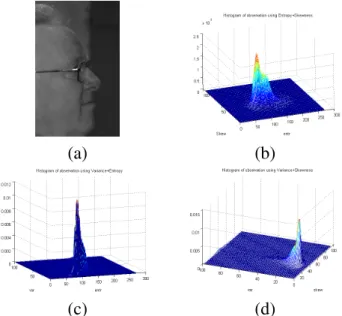
noise of standard deviation 20 (b) Joint distribution (skewness, entropy) (c) Joint distribution (entropy, variance) (d) (b) Joint distribution (skewness, variance) . . . 58 3.3 Example of feature distribution for a an image corrupted by real digital camera
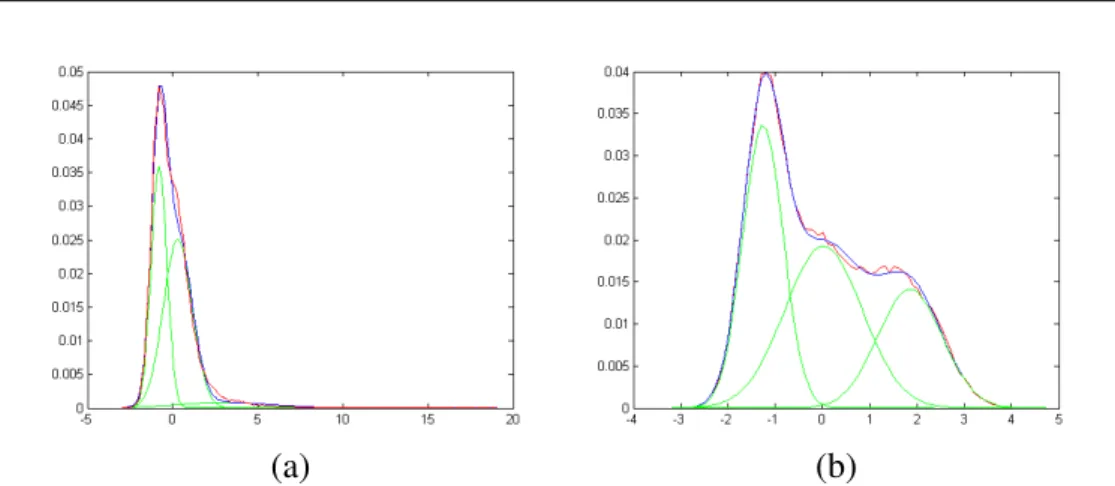
noise (b) Joint distribution (skewness, entropy) (c) Joint distribution (entropy, vari-ance) (d) (b) Joint distribution (skewness, varivari-ance) . . . 58 3.4 Histogram of the projection of the features vector on the first principle component
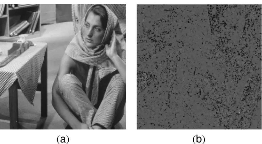
(red) and their approximation with Gaussian mixture models (blue) for (a) Old man image with real camera noise (b) Barbara image . . . 62 3.5 Results of an image partition: (a) original image, and conditional probability
func-tion relative to (b) ”smooth component” p(ox|smooth) , (c) ”texture” p(ox|tex) and (d) ”edges” p(ox|edge) . . . 63 3.6 Results of an image partition: (a) original noisy image (σn=20), and conditional
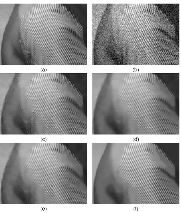
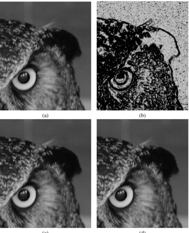
probability function relative to (b) ”smooth component” p(ox|smooth) , (c) ”tex-ture” p(ox|tex) and (d) ”edges” p(ox|edge) . . . 64 3.7 Zoom on a detail in the Barbara image (a) original image (b) noisy image (c)
restoration results using our technique with variable bandwidth kernels (d) restora-tion results using our technique with fixed bandwidth kernels (e) restorarestora-tion result obtained with NL-means algorithm (f)restoration result obtained with UINTA al-gorithm . . . 75
16
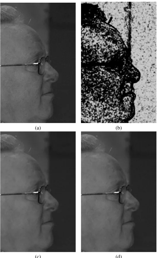
3.8 Results of our proposed denoising method on real digital camera Noise, (a) orig-inal image (b) variable bandwidth function (low intensity (hy=2), high intensity
(hy=4)) (c)MPMf ix denoising, (d) MPMvardenoising. . . 76 3.9 Results of our proposed denoising method on real digital camera Noise, (a)
orig-inal image (b) variable bandwidth function (low intensity (hy=2), high intensity
(hy=4)), (c)MPMf ixdenoising, (d) MPMvar denoising. . . 77 3.10 Results of our proposed denoising method on real digital camera Noise, (a) original
image (b)MPMf ix denoising, (c) MPMvar denoising. . . 78 4.1 Overview of ”Random Walks” based image enhancement. . . 83 4.2 Two pdf distributions pµ,σ(d) for different values of µ and σ (top (µ = 39, σ =
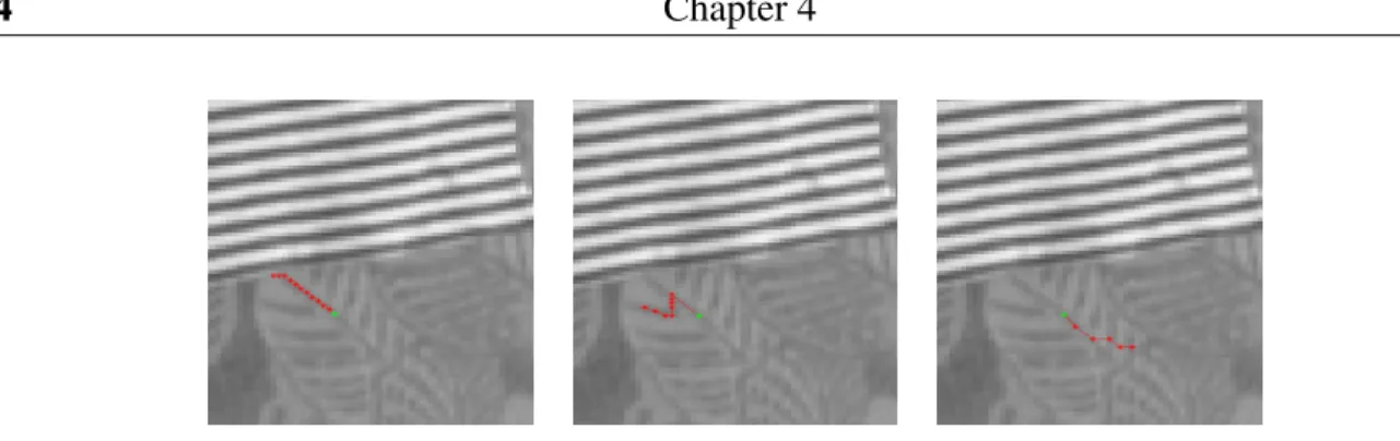
11.67), bottom (µ = 96, σ = 3.55), and sample generation according to these pdf (red pixel) for two different positions . . . 85 4.3 Illustration of systematic resampling scheme . . . 90 4.4 Example of three particles walks (red pixel) starting from the same origin position
(green pixel), the walks follow image structure. . . 94 4.5 (a) Noise free image (b)Image corrupted with Gaussian noise σn = 20 (c) Bilateral
filter restoration (d) Residual of the bilateral filter. . . 99 4.6 (a) Restoration result obtained with NL-means algorithm (b) NL-mean residual (c)
Restoration result obtained with random walks algorithm (L2 distance) (d)
Resid-ual of the random walk based approach . . . 100 4.7 (a) Restoration result obtained with random walks algorithm (Sobolev distance)
(b) Residual of the random walk based approach (c) Restoration result obtained with KB06 [76] (d) KB06 [76] residual . . . 101 4.8 Zoom on the Baboon image (a) Original image (b) Noisy image (c) Bilateral filter
restoration (d) NL-Means restoration (e) Random walk restoration (f) Adaptive window size restoration. . . 102 4.9 Zoom on the fingerprint image (a) Original image (b) Noisy image (c) Bilateral
filter restoration (d) NL-Means restoration (e)Adaptive window size restoration (f) Random walk restoration. . . 103
17 4.10 (a) Original Lena image (b) image corrupted by speckle noise with variance σn =
0.025 (c) Random walk based restoration result (d) Total variation minimizing based restoration [7] . . . 105 4.11 (a) Original Baboon image (b) image corrupted by speckle noise with variance
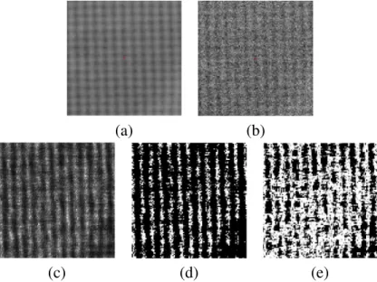
σn = 0.025 (c) Random walk based restoration result (d) Total variation minimiz-ing based restoration [7] . . . 106 5.1 (a) Original image (b) The bandwidth value associated to it . . . 121 5.2 (a) Example of texture (b) Texture corrupted by Gaussian noise σ2
n = 20 – Simi-larity measure between the central pixel (Red) and the other one using : (c) Using definition (5.16) and the noisy image (d) Using definition (5.33) and the noisy im-age (patch size d = 81) (e) Using definition (5.33) and the noisy imim-age (patch size
d = 25) . . . 124
5.3 Eigenvectors obtained through PCA decomposition of Barbara image corrupted by Gaussian noise (σn = 10) (patch size 15 × 15) (Only the first 22 component are significant if T=3) . . . 126 5.4 (a) Projection of the observations set on the first eigenvector of Barbara image
(b) Projection of the observation set on the 17th eigenvector (c) Projection of the observations set on the Last eigenvector (49th) . . . 127 5.5 (a) Example of texture (b) Texture corrupted by Gaussian noise σ2
n = 40 – Simi-larity measure between the central pixel (Red) and the other one using : (c) the L2
distance between patches (d) feature set based on PCA (e)the L2distance between
patches using the noise free image . . . 127 5.6 Zoom on the Barbara image (a) Original image, (b) Noisy image (c) Our method
using fixed bandwidth (d) Our method using variable bandwidth (e) Non local functional minimizing (5.9) (f) Total variation minimizing with variable local con-straint . . . 130 5.7 Zoom on the Barbara image (a) Total variation (b) Anisotropic Diffusion . . . 131 5.8 Zoom on the Lena image (a) Original image, (b) Noisy image (c) Our method using
fixed bandwidth (d) Our method using variable bandwidth (e) Non local functional minimizing (5.9) (f) Total variation minimizing with variable local constraint . . . 132
18
5.9 Zoom on the Lena image (a) Total variation (b) Anisotropic Diffusion . . . 133 5.10 (a) Residual of the Barbara image using the non local convex functional 5.9 (b)
Residual of the Barbara image using our approach with fixed bandwidth (c) Resid-ual of the Lena image using the non local convex functional 5.9 (d) ResidResid-ual of the Lena image using our approach with fixed bandwidth . . . 134 5.11 Zoom on Barbara image and result of our method using different weights
defini-tion and fixed bandwidth (a) using distance between pixels features using PCA (b) using the statistical distribution of the L2 distance between patches and expression
(5.33) (c) using L2distance between patches and expression . . . 135
5.12 Zoom on Lena image and Result of our method using different weight definition and fixed bandwidth (a) using distance between pixels features using PCA (b) us-ing the statistical distribution of the L2 distance between patches and expression
(5.33) (c) using L2distance between patches . . . 136
5.13 Results using NL-means algorithm (a) Original image (b) Noisy image (c) using the statistical distribution of the L2distance between patches and expression (5.33)
(d) The corresponding residual image . . . 137 5.14 Results using NL-means algorithm (a) using L2 distance between patches (b) Its
corresponding residual image (c) using distance between pixels features using PCA (d) Its corresponding residual image . . . 138 5.15 (a) original image (b) Noisy image. Results using NL-means algorithm (c)
us-ing L2 distance between patches (d) using distance between pixels features using
PCA (e) using the statistical distribution of the L2 distance between patches and
expression (5.33) . . . 139 5.16 Evolution of the PSNR value with respect to the retained number of principle
com-ponent . . . 140 5.17 Evolution of the PSNR with respect to the window radius : blue curve corresponds
to the classical weight definition (5.16) , the red curve corresponds to the new definition (5.33) . . . 140
19 6.1 (a) Macbeth Color Checkers (b) Curve corresponding to the evolution of the
stan-dard deviation of the noise with respect to the intensity for each channel Red ,Green and Blue . . . 147 6.2 Example of a raw Image with the Bayer Pattern . . . 147 6.3 (a) Original noisy image (b) Image restored using our method with fixed noise
variance (c) Image restored using the NLmean algorithm (d) Image restored using our method with variable noise variance . . . 151 6.4 Difference between the noisy image and the restored one using (a) our method with
fixed noise variance (b) Image restored using the NLmean algorithm (c) Image restored using our method with variable noise variance . . . 152 6.5 (a) Original noisy image (b) Image restored using our method with fixed noise
variance (c) Image restored using the NLmean algorithm (d) Image restored using our method with variable noise variance . . . 153 6.6 Difference between the noisy image and the restored one using (a) our method with
fixed noise variance (b) Image restored using the NLmean algorithm (c) Image restored using our method with variable noise variance . . . 154 6.7 Tensors on a volume slice (Homogeneous tensor field): (a) Noisy tensors (b)
Ground-truth (c) Result obtained with [43] (d) Result obtained with our method . . 162 6.8 Tensors on a volume slice (helix): (a) Noisy tensors (b) Ground-truth (c) Result
obtained with [43] (d) Result obtained with our method . . . 163 6.9 A slice of the T1-weighted volume, different muscle groups segmented manually . 164 6.10 Estimated tensors without regularization, tensors obtained with our method . . . . 164 6.11 (a-1) Image (Sythetic1) corrupted by the speckle σn= 0.5 (a-2) Image (Sythetic2)
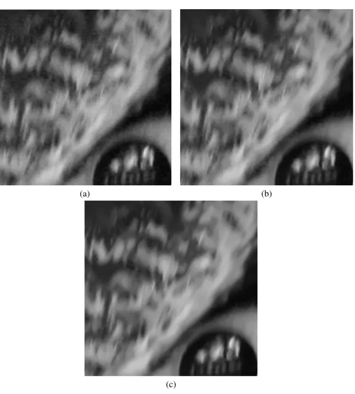
corrupted by the speckle σn = 1 (b) Result using the anisotropic diffusion [154] (c) Result using the wavelet based technique [116] (d) Result using our algorithm . 172 6.12 Results of restoration on real ultrasound frames. (a) Observed image (b) Result
20
6.13 Results of filtering real ultrasound frames (a) Observed image (b) Result of our algorithm without temporal component (Tw = 0) (frame by frame filtering) (c) Result of our algorithm using temporal filtering (Tw = 2) (d) Residual obtained with our algorithm without temporal component (Tw = 0) (frame by frame filter-ing)(e) Residual obtained with our algorithm using temporal filtering (Tw = 2) . . . 173 7.1 Results of Barbara image restoration (a) using Random walks (b) using MPM
es-timation with variable kernels bandwidth (c) using functional minimization based approach with variable bandwidth spatial kernel . . . 178 7.2 Results of Baboon image restoration (a) using Random walks (b) using MPM
es-timation with variable kernels bandwidth (c) using functional minimization based approach with variable bandwidth spatial kernel . . . 179 8.1 R´esultat de la restoration de l’image Barbara (a) En utilisant les marches al´eatoires
(b) En utilisant l’estimation MPM et les noyaux de taille variable (c) Minimisation de fonctionnelle en utilisant des noyaux de taille variable . . . 184 8.2 R´esultat de la restoration de l’image Baboon (a) En utilisant les marches al´eatoires
(b) En utilisant l’estimation MPM et les noyaux de taille variable (c) Minimisation de fonctionnelle en utilisant des noyaux de taille variable . . . 185
Chapter 1
Introduction en Franc¸ais
La restauration est l’un des composantes fondamentales du traitement des images. Cela consiste `a d´eterminer une image sans bruit `a partir d’une observation corrompue. Dans ce contexte, on doit consid´erer trois aspects importants qui sont (i) une mod´elisation ad´equate de l’image et du bruit (ii) une mod´elisation de la g´eom´etrie de l’image et des interactions entre les pixels (iii) la s´election de la fonctionnelle qui encode les mod`eles image et bruit ainsi que les interactions entre pixels afin de calculer l’image d´ebruit´ee. Dans la suite nous pr´esenterons le contexte de ce travail ainsi que les motivations et les principales contributions.
1.1 Pr´esentation du probl`eme et Motivations
On assiste de nos jours `a une prolif´eration d’images num´eriques dans la vie de tous les jours `a travers de nombreuses applications telles que la photographie, l’imagerie m´edicale, la vid´eo sur-veillance, la navigation et le contrˆole industriel, etc. Malgr´e le progr`es important r´ealis´e durant les derni`eres ann´ees par les constructeurs de cam´eras au niveau de la qualit´e des images, ces derni`eres ont besoin d’une ´etape de pr´etraitement avant son exploitation. Le besoin d’un compromis entre la qualit´e de l’image et le prix des cam´eras, ainsi que le renforcement de la concurrence entre les constructeurs pour produire des cam´eras `a moindre coˆut rendent les solutions logicielles attrac-tives. Ainsi, les applications de restauration des images telles que le d´ebruitage le d´eflouage et le inpainting ont attir´e beaucoup d’attention dans la communaut´e de la vision par ordinateur et le traitement des images. Parmi les diff´erents types de d´egradations, nous allons particuli`erement nous int´eresser `a la suppression de bruit.
22 Chapter 1
nombre de photons qui atteint un ´el´ement de capteur ou photosite durant une p´eriode T. Le bruit correspond alors `a la fluctuation du nombre de photons par rapport `a la moyenne qui correspond `a la vraie intensit´e. La chaleur d´egag´ee par le dispositif ´electronique est une source de bruit suppl´ementaire en g´en´erant des photons qui affectent chaque photosite et produisent le ”bruit d’obscurit´e”. D’autre part, chaque photosite g´en`ere du bruit qui peut contaminer les pixels voisins. Plus g´en´eralement, on peut approximer la relation entre l’image observ´ee I qui est mesur´ee par le capteur et l’image sans bruit U pour chaque pixel x par
I(x) = U(x) + n(x) (1.1)
o`u n est un bruit qui d´epend du pixel et qu’on assume blanc et de moyenne nulle. Le bruit blanc est caract´eris´e par l’ind´ependance entre ses diff´erentes r´ealisations.
Ainsi, le d´ebruitage est l’estimation de l’image U `a partir d’une observation bruit´ee I et de certaines hypoth`eses sur le mod`ele de bruit. Pour r´esoudre ce probl`eme, diverses m´ethodes ont ´et´e propos´ees au cours des cinq derni`eres d´ecennies. Malgr´e les progr`es importants r´ealis´es de nombreux d´efis doivent encore ˆetre soulev´es. L’efficacit´e d’un algorithme de d´ebruitage est li´ee `a sa capacit´e de pr´eserver les informations incluses dans l’image tels que les bords, la texture et les petits d´etails. Alors que la contrainte de pr´eservation du contour a ´et´e respect´ee par la plupart des algorithmes non lin´eaires de d´ebruitage, un effort doit encore ˆetre consacr´e au d´ebruitage de la texture. Cela est dˆu au fait que la plupart des algorithmes de d´ebruitage supposent que l’image est constante par morceaux. Une telle hypoth`ese n’est pas ad´equate avec les caract´eristiques des images naturelles qui peuvent contenir certaines structures aussi oscillantes que le bruit. De nombreuses recherches pour la mod´elisation de la texture ont ´et´e men´ees, mais leur efficacit´e est d´ependante de la taille de la texture ainsi que de sa structure. Ce dernier point rend pertinents les efforts consentis afin de trouver des mod`eles d’image plus r´ealistes et des algorithmes de d´ebruitage qui pr´eservent mieux la texture.
1.2 Les Contributions
Le travail pr´esent´e dans cette th`ese est un pas vers une meilleure compr´ehension des images et de la texture dans le but de d´eruitage. L’objectif principal est d’adapter au contenu de l’image les mod`eles utilis´es dans la restauration. Dans cette dissertation, nous pr´esenterons des mod`eles math´ematiques et les solutions num´eriques qui utilisent l’information appris `a partir de l’image observ´ee afin de construire une approche appropri´ee de d´ebruitage. Notre principale motivation est de concevoir une technique qui utilise des mod`eles d’images diff´erents selon le contexte local.
1. INTRODUCTION EN FRANC¸AIS 23 Cette th`ese pr´esente de nouvelles approches th´eoriques dans le but de d´ebruiter des images tout en pr´eservant la texture. Dans un premier temps, nous nous int´eresserons aux aspects photom´etriques du probl`eme dans le but de d´efinir des mod`eles appropri´es capables de d´ecrire l’observation et l’´echelle des interactions photom´etriques entre les pixels. Ensuite, nous allons ´etudier l’importance de la g´eom´etrie dans la d´efinition des d´ependances entre les pixels et par cons´equents dans les interactions spatiales ente eux. Le dernier volet de la th`ese consiste en deux contributions, un terme de r´egularisation plus g´en´eral qui permet de prendre en compte la complexit´e de l’image ainsi qu’une m´ethode automatique de s´election de la taille de la bande passante spatiale. Dans cette derni`ere partie nous nous int´eresserons ´egalement `a la d´efinition des poids qui r´egissent les interactions entre les pixels en fonction du contenu de l’image.
Notre premi`ere contribution consiste `a introduire la notion de classification dans le processus de d´ebruitage en utilisant des descripteurs locaux. Plusieurs techniques cherchent `a s’adapter au contenu de l’image en prenant en compte les caract´eristiques de chaque pixel pendant le d´ebruitage. Mais, certaines textures ont les caract´eristiques similaires au bruit ce qui empˆeche l’algorithme de restauration de les d´etecter. Pour cette raison, nous pensons qu’une ´etape de pre classification qui fourni un outil plus robuste pour identifier les zones textur´ees dans l’image est n´ecessaire. Cette classification consiste `a partitionner l’image en des r´egions localement lisses, des r´egions textur´ees et des contours. Ceci est effectu´e `a l’aide d’une classification dans un espace engendr´e par les caract´eristiques locaux qui permettent de d´ecrire les zones homog`enes, la texture et les contours. La projection des observations de cet espace dans un autre sous espace est mod´elis´ee par une mixture de Gaussienne o`u chaque composante est associ´ee `a chaque classe de pixels. Par la suite, le r´esultat de l’´etape de classification sera int´egr´e dans l’algorithme de d´ebruitage. La technique de filtrage s’appuie sur une technique non param´etrique avec des noyaux afin d’estimer le mod`ele image. Dans ce contexte, nous allons proposer une m´ethode automatique de s´election de la taille de ces noyaux qui d´epend du r´esultat de l’´etape de classification. En effet, dans le processus de filtrage nous traitons les pixels diff´eremment selon leur degr´e d’appartenance `a l’une des trois composantes de l’image. Ce dernier point est la contribution majeure par rapport aux techniques d´ej`a existante et qui utilisent pour mod´eliser l’image des techniques non param´etrique d’estimation de densit´e de probabilit´e [118, 10]. Contrairement `a ces m´ethodes, nous utilisons des noyaux de tailles variables qui d´ependent des propri´et´es locales du pixel.
La deuxi`eme approche ´etudi´ee dans cette th`ese est bas´ee sur les marches al´eatoires. Notre m´ethode explore plusieurs ensembles de voisins (ou hypoth`eses) qui peuvent ˆetre utilis´es pour le d´ebruitage d’un pixel, `a travers une approche de filtrage des particules. L’objectif est de proposer une m´ethode de s´election des pixels de l’image les plus pertinents qui vont ˆetre mis en jeu pour l’estimation de l’intensit´e d’un pixel donn´e. En s’appuyant sur une technique de filtre `a particules,
24 Chapter 1
la s´election des pixels se fait d’une mani`ere progressive. Nous consid´erons d’abord un voisinage de taille petite puis on ajoute de plus en plus de pixels en explorant le domaine de l’image tout en ´etant dirig´e par les structures. Contrairement aux filtres de voisinage classiques, le domaine consid´er´e lors du filtrage est adapt´e `a chaque pixel. Le processus de filtrage met en jeu un nombre de particules qui explorent le domaine de l’image en utilisant une distribution statistique qui d´ecrit la g´eom´etrie de l’image ainsi l’´etat d’une particule se r´ef`ere `a l’´etat du processus de reconstruction de l’image.
Les deux m´ethodes pr´ec´edentes permettent de restaurer l’image pixel par pixel. Bien qu’il s’agisse d’un moyen simple de restauration, un processus d’homog´en´eisation global o`u toute l’image est it´erativement mise `a jour doit ˆetre envisag´e. De plus, ces deux techniques incluent deux ´etapes : la caract´erisation de la texture et le filtrage. Pour faire face `a cette limitation, nous allons consid´erer un mod`ele d’image global qui encode implicitement la structure de l’image. Le d´ebruitage sera donc effectu´e `a l’aide de la minimisation d’une fonctionnelle quadratique et con-vexe qui implique aussi des noyaux `a taille variable. Ces noyaux sont utilis´es dans le calcul de similarit´es spatiales et photom´etriques entre les pixels. Afin de pr´eserver la texture et am´eliorer la qualit´e de l’estimation, nous allons consid´erer que l’´echelle des interactions spatiales est variable en fonction du pixel. Ceci permettra de l’adapter au contenu de l’image et `a l’´echelle de sa texture. La d´efinition d’une mesure de similarit´e appropri´ee qui soit plus robuste au bruit que la distance L2
entre les patches a ´et´e ´egalement ´etudi´ee dans cette dissertation. Cette distance est calcul´ee entre les vecteurs caract´eristiques qui sont obtenus par projection des patches de l’image dans un autre sous-espace permettant une meilleure description de la structure des patchs de l’image. De plus, nous avons propos´e une nouvelle d´efinition de poids qui est plus coh´erente avec la distribution statistique de la distance L2 entre les patchs de l’image.
Nous avons pr´esent´e dans cette th`ese plusieurs extensions de la technique de filtrage en min-imisant une fonctionnelle d’´energie convexe `a d’autres types de bruit et de donn´ee afin de montrer sa flexibilit´e. Cette extension concerne (i) la restauration des images en couleur o`u on doit prendre en consid´eration les propri´et´es du bruit relatif aux appareils photo num´eriques (ii) l’estimation et la r´egularisation des tenseurs de diffusion o`u les tenseurs doivent ˆetre d´efinis positifs (iii) filtrage des s´equences Ultrasonores o`u on adapte la formulation d’´energie `a la nature du bruit multiplicatif.
1.3 Plan de la th`ese
Cette th`ese est organis´ee comme suit: Le deuxi`eme chapitre est d´edi´e aux mod`eles non param´etriques d’estimation de densit´e de probabilit´e ainsi qu’aux techniques de partition de l’image. Au d´ebut,
1. INTRODUCTION EN FRANC¸AIS 25 nous allons pr´esenter un travail li´e `a cette technique qui est un filtre adaptatif non supervis´e (UINTA) et nous pointerons les diff´erences avec ce filtre. Par la suite, nous allons d´ecrire notre ap-proche de partition de l’image en trois classes ”r´egions homog`enes”, ”r´egions textur´ees” et ”con-tours”. Cette partition s’appuie sur le calcul de descripteurs locaux et la classification `a l’aide de mixture de Gaussienne. Apr`es l’´etape de classification nous allons nous concentrer sur le d´ebruitage. Nous allons passer en revue la th´eorie de la d´ecision Bayesienne et les diff´erents types d’estimateurs. Ensuite, nous allons pr´esenter notre technique de d´ebruitage utilisant une technique de Maximum a Posteriori Marginal (MPM) o`u on estime cette loi a posteriori `a l’aide d’une approche non param´etriques. Par la suite, nous nous int´eresserons `a la s´election de la taille du noyau et au processus de l’optimisation. L’´evaluation des performances sera pr´esent´ee `a la fin du chapitre.
Le troisi`eme chapitre sera d´edi´e aux filtres de voisinage et nous utiliserons une strat´egie bas´ee sur les marches al´eatoires et les filtres `a particule afin de s´electionner l’ensemble de pixel le plus adapt´e pour d´ebruiter un pixel donn´e. Au d´ebut, nous allons pr´esenter un mod`ele statistique qui permet de d´ecrire la g´eom´etrie de l’image et les relations spatiales entre les pixels similaires. Un tel mod`ele sera utilis´e dans le contexte du filtre `a particules afin de guider l’´evolution de ces derni`eres. Par la suite, nous pr´esenterons une description br`eve des techniques des filtres `a par-ticules. Nous allons ´egalement appliquer cette technique d’estimation pour restaurer des images aussi bien dans le cas de bruit additif que multiplicatif. Nous allons conclure cette section par la validation exp´erimentale de cette technique.
Dans le quatri`eme chapitre on va pr´esenter une technique de r´egularisation qui consiste `a min-imiser une fonction d’´energie convexe. Au d´ebut, on va commencer par pr´esenter l’´etat de l’art des techniques variationelle. Ensuite, nous allons nous int´eresser `a la description du mod`ele que nous utiliserons ainsi que le processus de diffusion sous-jacent. Apr`es la d´efinition du mod`ele, notre objectif sera la d´efinition des interactions entre les pixels. Cette interaction est r´egie `a l’aide d’une fonction de poids d´efinie par deux noyaux : un qui p´enalise la distance spatiale entre les pixels et l’autre la distance photom´etrique. Dans ce contexte nous avons essay´e d’am´eliorer la d´efinition des poids en optimisant la s´election de la taille du noyau spatial (celui qui g`ere les interaction spatiales entre les pixels) et en l’adaptant `a chaque pixel. Nous nous sommes ´egalement int´eress´es aux similarit´es photom´etriques entre les pixels et nous avons propos´e deux nouvelles d´efinitions de mesures. La premi`ere s’appuie sur une meilleure caract´erisation des pixels et la deuxi`eme exploite les propri´et´es statistiques de la distance L2entre patches. Finalement, nous conclurons ce chapitre
avec les r´esultats exp´erimentaux.
26 Chapter 1
autres que le probl`eme classique du bruit additif Gaussien et les images de niveau de gris. Au d´ebut nous allons consid´erer le probl`eme de filtrage des images en couleur corrompues par le bruit des appareils photo num´eriques. Pour cette application, nous allons discuter le mod`ele de bruit et proposer une technique non param´etrique d’estimation de la fonction de bruit. Cette fonction d´ecrit l’´evolution de la variance de bruit en fonction de l’intensit´e. Par la suite, nous introduirons la proc´edure de d´ebruitage des images en couleur `a l’aide de la minimisation sous contraintes de la fonction d’´energie pr´esent´ee dans le chapitre pr´ec´edent. La deuxi`eme application concerne des donn´ees de plus grandes dimensions sur des manifolds tels que l’exemple de l’imagerie des tenseurs de diffusion. L’objectif est d’estimer et de r´egulariser simultan´ement les tenseurs des diffusions `a partir d’images IRM. Les performances de cette m´ethode ainsi que son impact sur la classification des diff´erents muscles seront ´evalu´es. La derni`ere section est d´edi´ee `a la suppres-sion du Speckle dans des s´equences ultrasons. Pour atteindre cet objectif nous avons adapt´e le terme d’attache aux donn´ees ainsi que la d´efinition des poids au mod`ele du bruit. Les validations exp´erimentales de cette technique seront fournies a la fin de ce chapitre.
La conclusion et la discussion seront pr´esent´ees dans la derni`ere partie de ce document. Nous parlerons des limitations des diff´erentes approches propos´ees ainsi que les perspectives futures de ce travail.
Pour conclure, cette th`ese s’articule autour la mod´elisation des images et du bruit dans le con-texte de la restauration des images dans le domaine de la photographie num´erique ou l’imagerie m´edical. Cette th`ese a produit (jusqu’a maintenant), un chapitre de livre [109] quatres articles dans des conf´erences internationales de r´ef´erence [12, 15, 13, 11] deux articles dans des workshops [14, 110], et des articles de revue en cours (International Journal of Computer Vision, IEEE Trans-actions on Pattern Analysis and Machine Intelligence, Journal of Mathematical Imaging) ainsi qu’une implication dans un brevet franc¸ais [30].
Chapter 2
Introduction
Image restoration is one of the most fundamental components of image processing. It consists of recovering a noise-free signal from corrupted observations. Such a problem arises in a number of fields and has been heavily studied in the past decades. In such a context, one has to address three critical aspects, that are (i) appropriate modeling of the image towards understanding the noise level, (ii) appropriate modeling of the geometric dependencies between observations in the image domain and (iii) appropriate selection of a functional that encodes the previously mentioned com-ponents towards recovering the noise-free signal. In this chapter, we review the most representative techniques of the field, discuss their strength as well as their limitations in particular with respect to the above mentioned components.
2.1 Problem Statement and motivation
We witness currently the proliferation of digital images in every day life as well as in a number of industrial domains like photography, medical imaging, video surveillance, navigation, industrial inspection etc. Despite important progress made over the past decades from camera manufacturers on the quality of acquisition, these images need often a preprocessing step to be exploitable in a number of fields due to the need of a compromise cost versus quality. This is amplified due to the competition towards providing low cost cameras. Based on the assumption that conventional hardware sensors have reached a certain maturity, the investment needed to improve the quality of the images is disproportional to that improvement. This context favoured the emergence of soft-ware/algorithmic approaches toward image quality improvements. Therefore, image restoration application such as denoising, deblurring and inpainting gained a lot of attention from the
com-28 Chapter 2
puter vision and image processing community. Among all types of image degradations, we will focus in this thesis particularly on the noise suppression.
Let us introduce the problem using some standard conventions. Using conventional sensors, the observed image intensity for a given pixel corresponds to the number of photons that reach a cell of the light sensors matrix (called photosite) during a period T . The noise then refers to a fluctuation in the number of photons with respect to a mean value that is the actual intensity of the pixel. The heat generated by the electronic device is an additional noise source; it frees electrons that affects each photosite and gives rise to the ”dark noise”. On the other hand each photosite itself generates electrical noise that can contaminate its neighbor. In the most general case, one can approximate the relation between the observed image I measured by the sensor and the noise-free image U for each pixel x by
I(x) = U(x) + n(x) (2.1)
Where n is a pixel dependent additive noise that is often assumed to be white and of zero mean. The white noise is characterized by the independence between the random variables that correspond to noise realizations for two different pixels.
Hence, denoising refers to estimating the image U given the corrupted observation I and certain assumptions on the noise model. To address this problem various methods were proposed for the past five decades and despite important progress made many challenges are still to be dealt with. The efficiency of a denoising algorithm is related to its ability to preserve image content such as edges, texture and other fine details. While the contour preserving constraint was respected for the most non linear denoising algorithm, some effort has still to be devoted to texture denoising. This is due to the fact that most denoising algorithms are based on mathematical models describing the image as smooth or piecewise smooth. Such an assumption does not comply with natural image characteristics that may contain some structures that are as oscillatory as noise. Many research were also carried toward texture modeling but their efficiency depends on the scale of the texture and on its structure. The latter point makes relevant the effort dedicated to consider more realistic models and to design texture preserving denoising approaches. In this introduction we will briefly review the state of the art in the field and describe their underlying concepts. This review encompass neighborhood filters, Partial derivative, equation based regularization, sparse image representation, and Markov random fields models.
2. INTRODUCTION 29
2.2 State of the Art
Image processing and computer vision literature includes different kinds of algorithms to address image enhancement. To this end, a wide variety of mathematical tools was considered such as: signal approximation in sub-spaces, variational calculus, partial derivative equation, probability and statistics, information theory, etc. The definition of frontiers between the different available methods is not straightfoward. In many cases, one can find eminent links between different con-cepts like PDE’s based approaches and total variation minimization or neighborhood filters and wavelet thresholding with the Bayesian decision theory etc. Nevertheless we consider four cate-gories for image restoration techniques : (i) methods related to neighborhood filtering that consists in performing a weighted averaging (ii) PDE’s based approaches that are iterative techniques that yield a smoother version of the image with time. (iii) the sparse image representation and do-main transforms techniques which decompose the image into a sub-space where the image can be approximated by a few number of coefficients (iv) statistical methods and mainly the Markov Random Fields based approaches.
In order to introduce these methods, some basic definitions of the the underlying image repre-sentation are to be considered. We can find in the litterature three distinct forms to represent an image.
• Continuous model where the image is a function defined on a subset Ω ⊂ R2 called the
image domain and associates to each element of Ω a value in the set {0 . . . 255} for gray level images quantified and coded on 8 bits. In this case the pixel x ∈ R2is characterized by
the couple of its real coordinates.
• Discrete model where the image is defined on a discrete grid Ω ⊂ Z2 called the image
do-main and with values from the set {0 . . . 255} for gray level images quantified and coded on 8 bits. In this case the pixel x ∈ Z2 is characterized by the couple of its integer coordinates.
• Stochastic model where the image is assumed to be a sample of a random variable U = {U(xk)}1≤k≤|Ω|. U(xk) is a random variable that takes values in {0 . . . 255} and describes the intensity observed at a pixel xk.
30 Chapter 2
2.2.1 Averaging Based Filters
Averaging based filtering approaches are among the most primitive and the most widely used techniques in the field. The central idea is to reduce noise in the image by performing a weighted average of the other pixels in the image. A general formulation of such a filter is
U(x) = Z D h(x, y)I(y)dy and Z D h(x, y)dy = 1 (2.2)
Where D is the domain where the averaging is computed. It can be a local neighborhood of x or the entire image domain.
The selection of the function h is fundamental for the filtering process. The well known Gaussian filter is derived if h is a Gaussian function depending on the spatial distance between pixels. It is well known that the Gaussian filter and other linear ones result in blurred edges and fine details suppression. For this reason, non linear and data driven weighting functions were proposed to ensure better restoration. The underlying concept of these filters is to go further than the spatial distance between pixels to include other image features such as intensity. Despite an enormous volume of research literature in this field, we will focus on the most representative ones:
• The neighborhood filter
These filters performs a weighted average over a local neighborhood of x (noted Πx) where
the contribution of each pixel is dependent on the similarity between pixels. Earlier approach refers to the sigma filter [92] where a threshold on the intensity difference between neigh-boring pixel is considered to discard the irrelevant ones. In [153] a similar idea is expressed through the definition of weights coefficients depending on the gray level difference between pixels. The estimated intensity is written as
U(x) = 1 Z(x) Z Πx I(y)e− |I(x)−I(y)|2 σ2ph dy Z(x) = Z Πx e− |I(x)−I(y)|2 σ2ph dy (2.3)
σphis a parameter that controls the smoothing amount of the filter. Such a definition would preserve edges and other details since the neighboring pixels with an important intensity difference do not contribute in the reconstruction process (when compared with the σph). One can see a direct equivalence between this filter and the gaussian filter when σph value are important.
Recent equivalent formulations of this filter are the SUSAN Filter [127] and the Bilateral Filter [134, 112] that combine the spatial distance as well as photometric distance to compute
2. INTRODUCTION 31 the weights. These filters are defined as follows
U(x) = 1 Z(x) Z Ω I(y)e− kx−yk2 σ2s e −|I(x)−I(y)|2σ2 ph dy Z(x) = Z Ω e− kx−yk2 σ2s e −|I(x)−I(y)|2σ2 ph dy (2.4)
σs is a spatial parameter that defines the radius of the neighborhood considered for denois-ing. As in the former case, when σph is high this filter is equivalent to the Gaussian kernel smoothing.
This class of approaches combines computational efficiency (local operations) with satis-factory results. The main challenge refers to the appropriate definition of their parameters while at the same time, the computation of weights might be problematic when the images are heavily corrupted. This is due to the fact that simple pair-wise image intensities cannot encode the relation between the local observations. This was addressed by the NL-means algorithm.
• The Non Local means filter (NL-means) [26, 25]
The NL-means is an algorithm that takes advantage of the redundancy and similarity inside an image to perform denoising. Exploiting this natural image property was first used in case of texture synthesis in [51]. Based on this observation, the NL-mean weight function relies on a similarity measure that goes beyond pixel-wise resemblance and is determined through comparison of local image patches. Since similar patches can be found everywhere in the image (long edges, large textured regions with repetitive patterns), the spatial distance between pixels is neglected when considering the definition of the weight. The restored intensity obtained using the NL-means algorithm is given by the following expression
U(x) = 1 Z(x) Z Ω I(y)e− d(x,y) σ2ph dy Z(x) = Z Ω e− d(x,y) σ2ph dy (2.5) d(x, y) = Z R2 Gα(t) |I(x + t) − I(y + t)|2dt (2.6) Where Gα is a Gaussian kernel of bandwidth α that defines the size of the window (or image patch) taken for pixel comparison while σphplays the same role as in the previously cited filters. The discrete formulation of the NL-means filter requires the definition of a neighborhood Nxand INx the observed intensities within this neighborhood.
U(x) = 1 Z(x) X y∈Ω I(y)e− kINx −INyk22 σ2ph Z(x) =X y∈Ω e− kINx −INyk22 σ2ph (2.7) With this definition the NL-means acts as a basic averaging with equal weights in flat
re-32 Chapter 2
gions, while performing anisotropic filtering for edges or texture.
The computational cost is a serious limitation for the NL-means algorithm, and this was addressed in [98]. Despite the excellent performance of this filter, the selection of the filter-ing window (pixels contribution in the process), as well as the similarity measure between patches (both in terms of the choice of the metric and the contributing content) are two open issues. This was partially addressed in [76] where the idea of adaptive/variable filter bandwidth was considered.
• Variable neighborhood size filters
These are algorithms where the size of the domain D over which the mean is computed depends on the pixel position. The optimal window size is determined according to a trade off between variance and bias of the intensity estimator using local averaging [52, 117, 93, 76]. The most recent contribution in this area was presented in [76]. The authors suggest an alternative approach to the NL-means algorithm where the optimal filter bandwidth is computed for each pixel. To give an overview of this method, let us consider a local or semi-local version of the NL-means algorithm. The estimated intensity for a given pixel x is
ˆ U(x) = X y∈Dx I(y)wxy with wxy = e− d2(INx ,INy ) σ2ph P y∈Dxe −d2(INx ,INy )σ2 ph (2.8) d2(I
Nx, INy) is the L2 distance between patches.
Now if one considers the error expectation between the estimated intensity and the actual noise free one, the following relation is obtained
Eh( ˆU(x) − U(x))2i= b2
x+ vx2 (2.9)
with bx1being the bias of the estimator that characterizes the accuracy of the approximation
of the image at the pixel x using the local neighborhood Dx. The variance of the estimator vxcorresponds to the amount of fluctuation around the mean value of the estimator.
Ideally the perfect estimator is the one that minimizes both bias and variance which are com-peting variables. Assuming that the bias is increasing with the size of Dxand the variance is
decreasing, there exists an optimal size of Dxfor which a balance between the variance and
bias is reached. A direct estimation for this optimal size is not possible since the bias is not available. As an alternative, the author introduced in [76] a data driven window size selector. The underlying key idea is the following : if one considers ˆUp(x) and ˆUq(x) two estimates 1b
x= U (x) − E( ˆU (x)) ≈ U (x) − P
2. INTRODUCTION 33 of U(x) using two windows Dp
xand Dxq of size p and q respectively (p < q) smaller than the
optimal size value, then it was proved in [75] that ¯
¯
¯ ˆUp(x) − ˆUq(x)¯¯¯ ≤ κvp
x (2.10)
This observation provides an automatic technique to determine the optimal window size that is defined as: Argmaxq n q = |Dxq| such that ¯ ¯ ¯ ˆUp(x) − ˆUq(x) ¯ ¯ ¯ ≤ (2γ + κ)vxp ∀ 1 ≤ p ≤ q o (2.11) The optimal window is the largest one such that the estimators ˆUp(x) and ˆUq(x) are not too different, for all 1 ≤ p ≤ q . Hence, if an estimated intensity using a given window size is far from the intensity value provided by a smaller one, this means that the bias is already too large. In this case a smaller size has to be selected.
A crucial parameter for this method is the threshold κ because a large value of κ yields a large window size when small values favor small windows. For the selection of this para-meter the authors use a prior on the image and design their selection process such that high
κ values are set for smooth area and smaller one when discontinuities are observed. This
algorithm improves substantially the performance of the basic NL-means.
To conclude, we can say that these methods are attractive and simple to implement. Nevertheless one can seek further improvements by adapting in an automatic fashion the shape of the domain D as well as its size.
2.2.2 PDE’s and Energy Based Image Restoration
Over the past decades the image analysis field has seen the emergence of several PDE based mod-els. Image regularization is a field that has largely benefited from these techniques. In such a context, images are considered as evolving functions of time. Within this framework, the final solution of the enhancement process will correspond to the steady-state of the PDE. Such partial differential equations can be either determined through certain expected geometric constraints or can be the outcome of the minimization of a specifically designed cost function. In this section we will review the most classical ones.
34 Chapter 2
• Geometric Flows and Image Enhancement or axiomatic PDE’s
The earlier contributions in this field were linear PDE’s where the blurring is spatially in-variant [151, 85]. For instance, the heat equation is an isotropic filtering and is defined as
∂U
∂t = c∆U (2.12)
Where c is a constant and ∆ is the Laplacian operator. In [85] it was proved that performing an isotropic diffusion with c = 1 amounts to applying a convolution with a Gaussian kernel
Gσ = 2πσ1 exp(−kxk
2
2σ2 ) with a standard deviation σ =
√
2t. The isotropic diffusion blurs the image little by little which is a major drawback in denoising applications.
This issue was partially addressed by anisotropic diffusion, that is an alternative PDE’s based formulation aiming at preserving edges being present in the image. In [115] a paradigm that respects image discontinuities by considering a spatial varying c function instead of the constant one is presented. The underlying PDE is defined using the divergence operator
∂U
∂t = div(c(x, t)∇U) (2.13)
To preserve discontinuities the diffusion is conditioned by an appropriate choice regarding the c function. Such a function should favour diffusion in smooth regions and stop it near image boundaries. The use of a function that is decreasing with respect to the norm of the image gradient is a natural selection. In this context, two functions with similar properties and performance were proposed: c1(|∇U|) = exp(−|∇U |
2
K2 ) and c2(|∇U|) = 1
1+|∇U |2K2 with K a constant that can be assimilated to a gradient threshold. In [22], the author proposed
several choices of the c function inspired by the robust estimation framework and discussed the difference between them. An interesting method to understand the behavior of a given PDE is to consider its effect on the gradient direction η = ∇U
|∇U | as well as the tangential direction noted ξ. In [87], the authors provided some constraints on the diffusion along these two direction toward better edge preserving. Based on the same observation, other non linear PDE’s that aim to restrict the diffusion process only along the tangential direction to the gradient and tuned by the gradient magnitude were suggested [5, 78, 108]. For instance, in [5] a model that considers rather a smoothed version of the image gradient was considered.
∂U
∂t = g (|G ∗ ∇U|) |∇U| div ∇U
|∇U| = g (|G ∗ ∇U|) Uξξ (2.14)
Where g is a positive decreasing function and Uξξ is the second derivative of the image in the direction ξ. Such a model respects better the image features because it involves larger
2. INTRODUCTION 35 neighborhood while performing the diffusion along the tangential direction.
Other group of PDE operators are those that act directly on the level line of the image. The curvature motion is an interesting example of diffusion where the contrast invariance requirement is ensured [4, 155, 101]. The associated PDE is
∂U
∂t = F (curv(U), t) |∇U| (2.15)
Where curv(U) = div∇U
|∇U |refers to the curvature of the level line of U and F is an increasing function with respect to the first argument. The diffusion is performed along the normal direction to the level line and modulated by the curvature which leads to a curve shortening. Diffusion tensors (i.e. symmetric and positive definite 2× 2 matrices) based formalism, provides more generic framework. These formulations rely on the definition of a tensor field that imposes the direction of the smoothing. A general form of such a technique is presented in [145, 146, 149] where the evolution defined by a tensor D is
∂U
∂t = div(D∇U) (2.16)
The authors set the diffusion tensor to the structure matrix defined as D = (∇U∇UT) ∗ G σ. The diffusion is done according to the eigenvectors of the matrix D. For homogeneous regions this tensor is isotropic which yields a smoothing in all directions. Along image contours the diffusion is directed by the eigenvector that corresponds to the contour direction. Notice that considering a non local gradient direction estimation maintains coherence in the gradient direction for neighboring pixels which is an important issue in case of noisy images. Another unifying formulation of common diffusion equations that is based on the definition of diffusion tensors was proposed in [135, 137, 48]. It is based on the trace operator and the Hessian matrix H and is expressed as
∂U
∂t = trace(DH) (2.17)
this formalism allows the design of a specific smoothing that respects better the natural regularization properties than the divergence based model. The strength of tensor diffusion based formalism lies in the fact that it separates the design of the diffusion tensors from the smoothing process itself. Based on this property, one can retrieve the geometry of the structure in the image and then perform smoothing based on the computed tensor field.
• Energy-based Approaches
frame-36 Chapter 2
work. A smooth version of a noisy image is obtained by minimizing a cost function that penalizes the amount of variation in the image [86, 148, 122]. Earlier work refers to the total variational minimization that was first introduced by Rudin, Osher and Fatemi [122, 121]. They provided an edge preserving restoration approach by minimizing the L1 norm of the
magnitude of the image gradient. This problem is defined in the space of bounded varia-tions funcvaria-tions in Ω (BV (Ω) =©f ∈ L1(Ω)|R
Ω|∇f | < ∞
ª
). The interesting aspect of the proposed regularization is the fact that discontinuous and non smooth solutions are possible. The classical formulation of the ROF model is
Uopt = Argmin Z Ω |∇U| dx (2.18) Subject to Z Ω (U − I)2dx = σn2 and Z Ω (U − I)dx = 0 (2.19)
The estimated image has to be smooth while its difference with observed image (called residual) must have the same properties as noise : zero mean and same variance σ2
n. One can relax these two constraints and consider instead this unconstrained problem where the minimizer of the following energy function is an estimate of the noise free image.
E(U) = Z Ω |∇U| dx + λ Z Ω (U − I)2dx (2.20)
The second component of the energy is the fidelity term and it constrains the solution to be similar to the observed image I while λ is a parameter that controls the trade off between smoothness and fidelity to the observations. For a given λ value the constraint (2.19) is not necessarily verified unless one devotes special effort to compute λ as done in [74, 122]. The functional (2.20) is strictly convex and in [33] the authors provided a proof of the existence and the uniqueness of the solution. The Euler Lagrange equation associated to this energy is the following: div µ ∇U |∇U| ¶ + λ(U − I) = 0 (2.21)
To solve this equation the authors proposed in [122] the use of artificial time marching which is equivalent to the steepest gradient descent of the energy function. The image is considered as a function of space and time and one has to find the steady state solution for the equation
∂U ∂t = div µ ∇U |∇U| ¶ + λ(I − U) (2.22) with div ³ ∇U |∇U | ´
2. INTRODUCTION 37 Based on this flow, the amount of the smoothing applied to an observation is related to the curvature of the level line passing through it. The edges are preserved because they have small curvature. Nevertheless details and other oscillatory components different from noise may also be suppressed.
A more general formulation for the total variation minimization can be expressed if one considers only the regularization flow as follows :
ˆ U = ArgminU µZ Ω Φ(|∇U|)dx ¶ (2.23) where Φ is a positive and increasing function defined on R. We recall that the connection of this formulation with PDE’s is established by the Euler-Lagrange equation and the introduc-tion of an artificial time parameter so that at the convergence the energy gradient is equal to zero. The resultant PDE to problem (2.23) is of the form
∂U ∂t = div · Φ0(|∇U|) |∇U| ∇U ¸ (2.24) Hence, for a particular choice of the Φ function, we find again some models introduced above. The isotropic diffusion is obtained when Φ(s) = s2 [133], The Perona Malik
cor-responds to Φ(s) = 1 − exp(−s2
K2) and the Rudin Osher Fatemi model discussed above is
defined by Φ(s) = s. Contrarely to axiomatic PDE’s where one can enforce the diffusion only on the tangential direction of the gradient, the functional minimization is less flexible. More explicitly, when considering the decomposition of the diffusion process according to the gradient direction and the tangential one, we can notice that the coefficients are depen-dent. To this end, a careful choice of the Φ function to favour diffusion on the tangential direction with respect to the normal one has to be made.
Total variation minimizing based approaches are among the most popular denoising tech-niques that gained a lot of attention and were extended over the years to address many image processing problems such as deblurring, inpainting, optical flow estimation, stereo recon-struction, etc. For a more comprehensive theoretical analysis of total variational minimizing using PDE’s we refer the reader to [86].
• The Beltrami Flow
The Beltrami flow is another tool towards image analysis and regularization which relies on representing the image as a 2D surface in the 3D space for gray scale image and higher dimensional spaces for multi valued images [80, 82, 81, 129]. Thus considering the image as an embedding map M : x → (x, U (x)), the authors propose to minimize with respect to
38 Chapter 2
corresponds to the image surface and in case of gray scale images it could simply be written as ˆ U = ArgminU µ E(U) = Z Ω d2σ q 1 + |∇U|2 ¶ (2.25) Performing a gradient descent for the area of the graph representing U leads to the following diffusion equation where each point of the image is moving according to the normal of the surface which enables image edges preservation
∂U ∂t = div q ∇U 1 + |∇U|2 (2.26)
In [129] the author provided a general framework that uses measures on maps between Rie-mannian manifolds and showed the connections between this approach and other anisotropic diffusion PDE’s.
At the end of this overview we want to point out that this is not an exhaustive presentation of PDE’s based image analysis and other interesting work can be found in [31, 135]. Multi-valued images and constrained PDE are also an active research area and one can refer to [135, 48] for a review of these approaches.
Finally to conclude we can say that PDE’s are an interesting tools for image analysis able of extract image content at different scales. Nevertheless, as far as denoising application is concerned their performance is limited. This is due to the presence of fine texture and structure in the image that has similar scale to the noise and cannot, in the most general case, be characterized by a simple feature as gradient direction or other limited local interactions. One can overcome this limitation through the introduction of more global methods, like for example image decomposition/representation in sub-spaces.
2.2.3 Image Transform and Compact Representation
Image decomposition on a specific basis or dictionary offers powerfull tool used in many image processing applications (compression, restoration, inpainting etc). Their aim to provide a compact image model where an image can be reconstructed using few number of elements. In this section we will present two main approaches
• Image transform and wavelet basis
fea-2. INTRODUCTION 39 ture extraction and modelling. Denoising is among the applications that could take advantage of this representation. The first attempts in this direction were presented in [152] where the spectral image content is analyzed in a local window ( Discrete Cosine Transform or local Discrete Fourier Transform) then modified and the inverse transform gives an estimate of the noise free intensity.The major breakthrough in this direction came with the introduction of the wavelet decomposition. Wavelet transform provides a signal representation that encodes space and frequency. Moreover, it has a high capacity of approximating a given signal by a small set of coefficients. It refers to an image decomposition on a set of functions composed of shifted and dilated versions of the wavelet noted ψ. A wavelet is a function in L2(R2)
localized in space and that satisfiesRR2ψ(x)dx = 0 and kψk = 1. Hence, if we note ψv,s
the wavelet obtained after a shift v and dilation s, the definition of the wavelet coefficients of I is Iw(v, s) = hI, ψv,si = Z R2 I(x)ψv,s(x)dx where ψv,s(x) = 1 √ sψ µ x − v s ¶ (2.27) A particular and interesting case of wavelets are the orthogonal wavelets that form an or-thogonal basis of L2(R2) defined as nψ
n,j = √12jψ
³
x−2jn
2j
´o
j∈Z,n∈Z2. Since the image is
defined on a finite domain, it can be expressed through an orthogonal basis using a finite set of coefficients [103]. The image is projected on two orthogonal subspaces, the first one corresponds to the details of the image at different scales, the second to the lower resolution of the image. This decomposition is expressed as follows
I = J X j=L+1 X n∈[0,2−j]2 hI, ψn,ji ψn,j+ X n∈[0,2−J]2 hI, φn,ji φn,j (2.28)
This decomposition involves two main terms the first refers to the detail being present in the image at different scales while the second corresponds to a coarse version of the image represented by the basis vector {φn,j}n.
Since the wavelet transform concentrates a lot of energy on few coefficients that correspond to the useful information in the image while the noise is represented by small wavelet coeffi-cients, a natural way to perform denoising in the wavelet domain is to perform a thresholding [103]. An estimate of U can be expressed as
ˆ U = J X j=L+1 X n∈[0,2−j]2 ρT (hI, ψn,ji) ψn,j+ X n∈[0,2−J]2 ρT (hI, φn,ji) φn,j (2.29)