1
Baby-Boom, Baby-Bust and the Great Depression
Andriana Bellou* and Emanuela Cardia**1
Université de Montréal
This version: November 2014 (First version: June 2014)
Abstract
The baby-boom and subsequent baby-bust have shaped much of the history of the second half of the 20th century; yet it is still largely unclear what caused them. This paper presents a new unified explanation of the fertility Boom-Bust that links the latter to the Great Depression and the subsequent economic recovery. We show that the 1929 Crash attracted young married women 20 to 34 years old in 1930 (whom we name D-cohort) in the labor market possibly via an added worker effect. Using several years of Census micro data, we further document that the same cohort kept entering into the market in the 1940s and 1950s as economic conditions improved, decreasing wages and reducing work incentives for younger women. Its retirement in the late 1950s and in the 1960s instead freed positions and created employment opportunities. Finally, we show that the entry of the D-cohort is associated with increased births in the 1950s, while its retirement turned the fertility Boom into a Bust in the 1960s. The work behavior of this cohort explains a large share of the changes in both yearly births and completed fertility of all cohorts involved.
Keywords: Baby Boom, Baby Bust, Great Depression, Added Worker Effect, Retirement,
Fertility
Département de sciences économiques, Université de Montréal, Pavillon Lionel-Groulx, Université de Montréal, 3150, rue Jean-Brillant, Montréal (QC) H3T1N8. Other Affiliations: *CIREQ and IZA, **CIREQ. Corresponding author: Andriana Bellou (andriana.bellou@umontreal.ca). The authors gratefully acknowledge financial support from SSHRC and FQRSC. We thank Fabian Lange, Martha Bailey, Robert Margo, Edson Severnini, Uta Shoenberg and participants at the Queens Economic History Workshop (2014), University of Bologna, University of Southampton and University College London for their helpful comments.
2
1. Introduction
It is still unclear what caused the unprecedented increase in fertility between 1946 and 1964, the official dates of the baby-boom: from the cohorts of women born between 1906 and 1910, to the cohorts born between 1931 and 1935, fertility increased by 40%. What is equally surprising is that the spectacular increase then evaporated within a decade. Women born between 1946 and 1950 had an average of only 2.22 children, lower than the average of the cohorts born between 1906 and 1910.
While most studies of the baby-boom have typically focused on completed fertility, annual fertility rates also evolved in a very particular way. Births began to soar in the early 1950s, levelled off between 1958 and 1960 and declined rapidly thereafter. Interestingly, the timing of the boom and bust is similar across women of different childbearing ages in the 1950s and 1960s. Even more intriguing: women born between 1936 and 1940 had on average more births in 1960, when 20 to 24 years old, than all other baby-boom cohorts, yet overall they had on average fewer children than the previous cohort born between 1931 and 1935 (3.02 versus 3.21). These facts suggest that something happened between the end of the 1950s and the beginning of the 1960s that led all cohorts to reduce births. Although there were two official recessions between 1957 and 1958 and between 1960 and 1961, they were both fairly mild and brief and overall the 1960s was a period of growth and economic prosperity.
In this paper we propose a new explanation of the baby-boom and baby-bust that fits the timing of the increase and decrease in both yearly births and completed fertility. Our explanation links the fertility boom-bust to the Great Depression. We show that the Great Depression drew into the labor market a group of young married women, 20 to 34 years old in 1930, henceforth called the D-cohort. In the following decades this same cohort either remained in the labor market or exited to re-enter as economic conditions improved. Its entry in the 1940s and 1950s was massive and decreased wages and employment opportunities for all women, including the very young. Lower wages, in turn, implied a lower opportunity cost of having children and hence a substitution effect that discouraged work and encouraged family formation. The (re-) entry of the D-cohort also coincided with a period of substantial economic expansion, greater job security for men and possibly rising male incomes. We argue that this positive income effect together with a weakened substitution effect (via lower female wages and lower employment) generated the dramatic increase in fertility observed during the Baby-Boom. Born between 1896 and 1910, women in the D-cohort retired in the late 1950s and throughout the 1960s. In 1970 they were 60 to 74 years old and few were still working. Their massive exit from the labor market freed positions and increased the opportunity cost of
3
having children for younger women. This explains why in a period of economic prosperity we witnessed both a boom and a bust.2
Our explanation links the fertility boom-bust to the Great Depression via a different channel than the well-known “relative income hypothesis” proposed by Easterlin (1961). Our mechanism is the labor market behavior of women who were of working age during the depression years. Easterlin hypothesis instead relies on a preference shift, whereby young women who grew up during the Depression had low material aspirations and responded to the post-WWII economic recovery with renewed optimism and a desire for larger families. This hypothesis has received less attention recently, partly because the cohort with the highest average birth rate was born between 1936 and 1940 and was too young to have been directly affected by the Great Depression. The behavior of this cohort is instead well explained by the labor market channel we propose. Jones and Schoonbroodt (2014) also link the boom-bust to the Great Depression. Using a Barro-Becker model with dynastic altruism, they show that a large decline in income (as during the Great Depression) leads to a decline in contemporaneous fertility and to higher transfers per child later on. As a result, the next generation increases both consumption and fertility.
WWII could seem the most obvious alternative explanation of the baby-boom, as this occurred soon after the return of soldiers from the war. From the official entry of the US into the war, 16 million men were drafted and it took three and half years for the war to end. This alone could have triggered a catch-up effect and a baby-boom. But could this have been sufficient to explain the observed baby-boom, which spanned nearly two decades, and the subsequent bust? More importantly, even if delayed fertility could explain the boom and bust, this should not affect completed fertility, while the latter increased substantially. It is possible, however, that the war affected fertility via other channels.
Doepke, Hazan and Maoz (2013) use a calibrated macro model to show that the large entry of women (45 to 55 years old in 1960) into the workforce during WWII could have crowded-out younger women with less experience and led to a large increase in births. Their model and simulations show the important role of labor markets for fertility. Evidence that is not consistent with the war crowding-out young women is provided by Fernandez, Fogli and Olivetti (2007). They show that WWII increased the proportion of men brought up by working mothers as well as the labor supply of their daughters, 25 to 29 years old in 1960.
2 Jones and Tertilt (2006) find a negative relation between income and fertility, which would explain most of the fertility decline in the late 19th and 20th century, but does not adequately explain the baby-boom that occurred during a period of prosperity. Our hypothesis suggests that this relation was altered due to a temporarily weaker substitution effect.
4
They also find no long term labor supply effects of WWII for the mothers themselves, 45 to 50 years old in 1960. Goldin and Olivetti (2013) show that WWII increased the participation of white married women, 25 to 49 years old in 1950 and 35 to 44 years old in 1960, but find no effects for older women. In addition, they show that this increase only applies to women with at least 12 years of schooling.3 In this paper, we also find that young women work more in high mobilization states in 1960 and no significant effects for older women (our D-cohort). Moreover, annual data from the Current Population Survey do not indicate a decline in the presence of 45 to 55 years old women in the labor market in the 1960s (Figure 6 in this paper). This suggests that their retirement cannot explain the baby-bust in the early 1960s. Our thesis is instead that an older cohort of women, 50 to 64 years old in 1960 and right at the time to retire, triggered a fertility boom and a bust by crowding-out and then crowding-in younger female labor market entrants.
Several other studies link the baby-boom to a decrease in the cost of raising children during the 1950s consistent with the quality-quantity tradeoff formulated by Becker (1960) and Becker and Lewis (1973). Greenwood, Seshadri and Vandenbroucke (2005) credit the dramatic transformations in home production since the early 20th century and the rapid diffusion of modern appliances in the 1940s and 1950s for freeing time and increasing the demand for children. Bailey and Collins (2011) using county data on appliances and fertility show, however, that the link between home technology and fertility is either negative or insignificant. Murphy, Simon and Tamura (2008) attribute the baby-boom to the suburbanization of the population and to the declining price of housing, as proxied by population density. Albanesi and Olivetti (2014) instead link the baby-boom to improvements in health that significantly decreased maternal mortality in the early 20th century. The baby-bust is attributed to increased parental investments in the education of the daughters as life expectancy of women increased. Although the first pill was released in 1960 and it took time till its broad use, Bailey (2010) shows that it accelerated the post-1960 decline in marital fertility and contributed to the baby-bust.4 Nevertheless, these explanations neither provide a unique mechanism for both the boom and the bust nor account for the quick reversal from the fertility boom to the bust that affected the yearly births of women of all ages.
This paper instead presents instead a “unified” explanation of the boom-bust that does
3 Goldin (1991), using the Palmer survey to examine the impact of WWII on women’s work between 1940 and 1951, finds evidence consistent with the view that the war did not greatly increase women’s employment. Acemoglu et al. (2004) find a strong positive relation between mobilization rates and women’s employment which, however, fades substantially with time (Figure10, their paper). This is also in line with the results in Fernandez et al. (2007).
4 Bailey (2006) shows that greater fertility control contributed to the increase in young unmarried women’s market work from 1970 to 1990. Bailey (2010) shows that the pill also played an important role in the baby-bust. Among other explanations of the bust, the introduction of divorce laws in the 1970s does not fit the timing of the reversal.
5
not rely on other mechanisms for the boom to turn into a bust. Moreover, it is consistent with the timing of the rise and fall in annual births as well as completed fertility and it also explains why fertility changed simultaneously across all women of childbearing age. While other factors influencing the effective cost of raising children, as highlighted in the aforementioned studies, may have contributed to the fertility changes over the 1950s and 1960s, our channel alone explains a large part of both the boom and the bust.
Our empirical strategy is twofold. It relies on 1) using several panels of micro data from 1920 to 1970 to examine the work patterns of women of different ages in response to economic conditions during the Great Depression and afterwards (first part of the paper), 2) constructing a measure of crowding-out and crowding-in to test whether the entry and exit from the labor market of the D-cohort can explain the boom/bust in yearly births and completed fertility (second part of the paper). One difficulty lies in how to consistently measure changes in economic conditions during the first half of the century. Unemployment is not available annually before 1961 while information on income is not available prior to 1929. The only measure we are aware of, that is both at state and annual level since the start of the century, is the ratio of commercial failures to business concerns (US Statistical Abstracts). This covers failures in all commercial businesses.
The first part of the paper uncovers a set of interesting facts. We show that the market entry of the D-cohort can be traced to the late 1920s and early 1930s and is significantly higher in states where the Depression was more severe. Interestingly, only married women increased their presence in the early phase. A potential explanation for their entry is an added
worker effect, whereby decreased family income and credit market constraints pushed women
into the workforce. Consistently with this interpretation, Finegan and Margo (1994) calculate that in 1940 the participation of women whose husbands were unemployed (and not on work relief), was 50% higher than that of women whose husbands were employed in the private sector.
Using the 1940-1950 and 1940-1960 census panels we present strong evidence that economic conditions in the 1930s had a lasting impact on the employment of the D-cohort and also affected much younger women who were just children in the 1930s. These are the women who had some of the highest birth rates in the 20th century. We find instead no lasting significant effects on the employment of men. In both sets of panels we consistently find an opposite entry/exit response for old/young cohorts, with the D-cohort solely entering the labor market and the young cohorts exiting in states with more commercial failures in the early
6
1930s.5 The same striking entry/exit pattern is further reinforced by the subsequent economic recovery. The negative impact of the Depression on the young cohorts can only be indirect as they were not of working age in the early 1930s, some not even born.
We also show that in states more severely affected by the Great Depression, the wages of all women were lower decades later. Lower wages reduced the opportunity cost of raising children and the incentive for young women to enter the workforce. We verify if the market entry of the D-cohort is a plausible explanation for these findings by using instead of failures during the Great Depression, the share of women in the D-cohort working in 1930. The results are consistent with the proposed channel: a higher share lowers the ratio of young women working in 1950 and 1960, as well as the wages of nearly all women in 1950 and 1960. We perform several falsification tests to insure that we are not picking up spurious correlation with the business cycle but find no such pattern in response to economic changes that preceded the Great Depression.
These findings are in line with aggregate life-cycle employment trends. Figure 1 plots work shares of women by age from 1930 to 1970. As can be seen, the employment of older cohorts, and in particular of the D-cohort, increased tremendously throughout the decades. In the 1930s and earlier, women tended to withdraw from the labor force after marriage and not to re-enter. This changed drastically afterwards, but the increase is even more remarkable between 1950 and 1960, well after WWII was over. For example, 39% of the women in the
D-cohort were working in 1960, while only 18.6% in that age bracket were working in 1940.
This also implies that a large number of women was about to retire in the 1960s. It is only then that the employment of younger cohorts increased.
0 0,1 0,2 0,3 0,4 0,5 0,6
Figure 1: Share of white women working by age and year
share of women working in 1930 share of women working in 1940 share of women working in 1950 share of women working in 1960
5 Also younger cohorts of married women entered the labor market between 1930 and 1940, but the link to the Great Depression weakens and is not significant in the 1940-1950-1960 panels.
7
In the second part of the paper we explore whether there is a link between the work behavior of the D-cohort and the fertility of the younger cohorts that contributed the most to the baby-boom and bust. To do this, we construct measures of the share of women in the
D-cohort entering or exiting the labor market in the 1950s and 1960s. First, we show that these
measures predict a decline (increase) in the work propensity of women 20 to 29 years old in 1960 (1970) relative to women of the same age in 1940, our base and pre-baby-boom reference point. Second, we show that these measures also predict significantly more births in the 1950s, and significantly fewer in the 1960s. In both cases these effects explain 30% to 67% of the increase and decline in yearly births. Finally, we study whether these measures can predict higher/fewer cumulative births by a certain age for women responsible for the boom and bust, relative to women in the same age brackets in the base year. We find similar results as for yearly births. Numerous falsifications are performed to assess whether by isolating the impact of one cohort, the D-cohort, we are not overestimating its impact. To address this issue, we examine the crowding-out and crowding-in impact of other cohorts. In all cases we find that the D- is the only cohort that produces such significant effects on births.
In the next-to-last section of the paper we discuss how other plausible mechanisms of the Baby-Boom fit within our framework. First, we consider the Easterlin hypothesis by explicitly examining the relative impact of economic conditions during childhood and adulthood on completed fertility. We do not find that relative improvements in the economic status of the Baby-Boom cohorts are associated with increases in their lifetime fertility. Second, we test whether the retirement of the D-cohort can account for the post-1960 sudden fertility change of the 1926-1940 Baby-Boom cohorts. The 1936-1940 “pivotal” cohort, for instance, had the highest average birth rate when 20 to 24 years old in 1960 but then drastically reduced its births within the next 5 years (see Figure 3 below). It would be difficult to reconcile these within-cohort own fertility switches with hypotheses that solely focus on changes in education or shifts in the preferences of the younger cohorts. We show, instead, that our mechanism can explain this fact.
Finally, in the last section of the paper, we use data on yearly birth rates and completed fertility for a sample of 18 countries, to test the impact of the Great Depression and WWII on fertility. Our estimates indicate that the Great Depression significantly increased and decreased births between 1949 and 1963 and led the cohorts born between 1925 and 1932 to have higher completed fertility and the cohorts born between 1942 and 1950, to have lower completed fertility. WWII, instead, has non-significant effects.
8
We proceed as follows. In Section 2, we describe the data and samples. Section 3 analyses the impact of economic conditions on work and wages. Section 4 describes our measures of crowding-out and crowding-in. Section 5 contains the main results on the impact of the crowding-out and crowding-in on the yearly births of different cohorts. Section 6 discusses their effect on cumulative births, Section 7 assesses alternative interpretations and Section 8 presents evidence on the role of the Great Depression on the fertility boom-bust across a sample of 18 countries. Section 9 concludes.
2. Data and Samples
Our main data sources are the 1% IPUMS files, between 1920 and 1970 (Ruggles et al., 2010), and the Statistical Abstracts of the United States. The first source is used to obtain micro-level information on the labor supply of women (and men), their fertility (annual and completed) and other demographic characteristics. The second source is used to collect temporal and geographic information on economic conditions. For this, we use state-level data on commercial failures and exploit differences in the extent of such failures within states over time and across states. This data was originally reported in Dun and Bradstreet Inc., NY. It is available on a state and yearly basis between 1900 and 1968. We plot the series by state and by the four census regions in Figure 2. As can be seen, there is considerable variation in the failure rate within and across states and over time but in general there are more failures in the early 1930s and very few during WWII. The economic boom of the 1950s, and to some extent of the 1960s, is also characterized by fairly low levels of business failures. Although we cannot use unemployment as a business cycle indicator due to data limitations, there are reasons to prefer commercial failures when examining the impact of economic conditions on labor markets.6 While unemployment is affected by shifts in both labor demand and supply, commercial failures are more akin to labor demand shifts that lead to layoffs than to labor supply shifts.
Fertility information from the IPUMS is exploited in two distinct ways. In the yearly fertility analysis, our strategy relies on comparing births in every year from 1950 till 1969 to births occurring in 1940 to women in the same age brackets. To compute yearly births in the 1950s and 1960s we use the 1960 and 1970 censuses respectively. We link young mothers up to 39 years of age in 1960 and 1970 respectively to their own children present in the household. The census reports the birth year of each family member in the household, and hence of all surviving children, which allows us to infer whether a woman gave birth in any of
6
Unemployment rate is reported every 10 years until 1960 by the census and can be calculated annually since 1962 from the Current Population Survey. Due to changes in the employment definition, however, unemployment rate estimates from the census before and after 1940 are not strictly comparable.
9
the intercensal years (1951, 1952 etc. and similarly 1961, 1962 etc.). We follow a similar procedure to infer births taking place in 1940.
Finally, our entire analysis focuses exclusively on white, native American women, not in group quarters. We further restrict attention to the ever-married when studying changes in completed fertility. Moreover, for sample comparability reasons across years, we produce our estimates using sample line weights as some of our core variables are only recorded for sample-line respondents (wages in 1950 and completed fertility in 1940-1950). Our results, however, are qualitatively and quantitatively robust to using person weights.
We choose 1940 as the base year as this precedes the baby-boom and also significant improvements in economic conditions. It also precedes WWII, which is one of the factors we take into account. Moreover, the year 1940 is a relevant reference point because women who were then 20 to 29 years old had nearly the lowest yearly and completed fertility since the beginning of the 20th century. Women instead who were 20 to 29 years old throughout the 1950s contributed the most to the baby-boom. Hence, our analysis is conducted to make more difficult the explanation of the change in births, from one of its lowest levels to the highest. In addition, prior to 1940 there are no individual data on wages and the definition of work is less comparable to the definition used for 1950 and 1960. For these reasons, to examine the impact of the D-cohort on work, wages and fertility within the same framework and assess the quantitative relevance of our mechanism, we chose 1940 as the base case throughout.7
7 Having said this, we experiment with 1910 as the base year for the fertility analysis and show that our results hold in the 1910-1960 and 1910-1970 panels.
Figure 2: Commercial Failures by Regions and States
Notes: Vertical axe: % Commercial failures per number of concerns in business by regions and states. Horizontal axe: year.
0 1 2 3 4 Northeast CT ME MA NH NJ NY PA RI VT 0 0.5 1 1.5 2 2.5 3 3.5 4 4.5 Midwest IL IN IA KS MI MN MO NE ND OH SD WI 0 0.5 1 1.5 2 2.5 3 3.5 4 4.5 West AZ CA CO ID MT NV NM OR UT WA WY 0 1 2 3 4 South AL AR DE DC FL GA KY LA MD MS NC OK SC TN TX VA WV
10
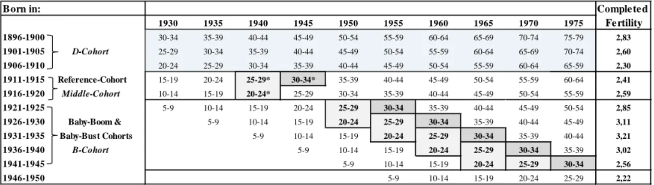
Table 1 shows the birth year of the cohorts included in the analysis and their ages between 1930 and 1975. We also report their average completed fertility (number of children ever born to white women aged 40 to 49 years old) on the right side of the table. We distinguish three broad cohort groups. The first is the D-cohort born between 1896 and 1910. The second is the Middle-cohort, our reference cohort, born between 1911 and 1920. The third, the B-cohort, includes all women who contributed to the baby-boom and bust; they were born between 1921 and 1945. The shaded light grey box between the D- and the B- cohorts highlights the age of the Middle-cohort in 1940, our base year (marked by a *) to which we compare changes in work and annual births in the 1950s and 1960s. We also highlight in light grey the cohorts that experienced the baby-boom and bust when 20 to 29 years old. These are the cohorts and age groups we focus on in our yearly fertility analysis. Finally, the cohorts whose cumulative fertility by age 30 to 34 we track over time are highlighted in darker grey. Women 30 to 34 years old in 1945 (marked by a *) are our reference point in that case. The B- and the D- cohorts are two groups removed from each other. Moreover, the reference cohort is neither part of the D-, nor part of the B- cohorts. This ensures that the results are not contaminated by within-cohort overlaps. The two-cohort cushion we keep between the D-cohort and the baby-boomers is justified by our finding of no persistent effects of the Great Depression on its entry into the labor market in the 1950s (see Section 3).
Table 1: Cohort Table
Born in: Completed
1930 1935 1940 1945 1950 1955 1960 1965 1970 1975 Fertility 1896-1900 30-34 35-39 40-44 45-49 50-54 55-59 60-64 65-69 70-74 75-79 2,83 1901-1905 D-Cohort 25-29 30-34 35-39 40-44 45-49 50-54 55-59 60-64 65-69 70-74 2,60 1906-1910 20-24 25-29 30-34 35-39 40-44 45-49 50-54 55-59 60-64 65-59 2,30 1911-1915 Reference-Cohort 15-19 20-24 25-29* 30-34* 35-39 40-44 45-49 50-54 55-59 60-64 2,41 1916-1920 Middle-Cohort 10-14 15-19 20-24* 25-29 30-34 35-39 40-44 45-49 50-54 55-59 2,59 1921-1925 5-9 10-14 15-19 20-24 25-29 30-34 35-39 40-44 45-49 50-54 2,85 1926-1930 Baby-Boom & 5-9 10-14 15-19 20-24 25-29 30-34 35-39 40-44 45-49 3,11 1931-1935 Baby-Bust Cohorts 5-9 10-14 15-19 20-24 25-29 30-34 35-39 40-44 3,21 1936-1940 B-Cohort 5-9 10-14 15-19 20-24 25-29 30-34 35-39 3,02 1941-1945 5-9 10-14 15-19 20-24 25-29 30-34 2,56 1946-1950 5-9 10-14 15-19 20-24 25-29 2,22
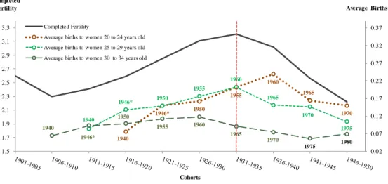
Figure 3 plots mean completed fertility by cohort (solid line) and the average births these cohorts had when 20 to 24 (dotted line), 25 to 29 (small dashed line) and 30 to 34 (long dashed line) years old in the years reported below or above the lines. The graph is rescaled: information about completed fertility is on the left and about births, on the right. Reading the graph vertically one can find the completed fertility of a given cohort and its average fertility rate at different points in time. The dotted (average births to 20 to 24 year-olds) and the small dashed lines (average births to 25 to 29 year-olds) cross over: earlier in the 1950s more children were on average born to 25 to 29 than to 20 to 24 years old women; later in the
11
1950s, this pattern is reversed. The change is striking for women born between 1936 and 1940. With respect to previous cohorts, they drastically decreased average births within few years of having had the highest average fertility rate. Our crowding-out and crowding-in hypothesis can reconcile the remarkable shift in the fertility of this same cohort.
gen baby=0
replace baby=1 if yngch<=1 gen baby2=0
replace baby2=1 if yngch<1
1940 1946* 1950 1955 1960 1965 1970 1940 1946* 1950 1955 1960 1965 1970 1975 1940 1946* 1950 1955 1960 1965 1970 1975 1980 0,02 0,07 0,12 0,17 0,22 0,27 0,32 0,37 1,5 1,7 1,9 2,1 2,3 2,5 2,7 2,9 3,1 3,3 Average Births Completed Fertility Cohorts
Figure 3: Completed Fertility and Yearly Births
Completed Fertility
Average births to women 20 to 24 years old Average births to women 25 to 29 years old Average births to women 30 to 34 years old
* In 1946 we take births of women in the same cohort but one year older
Finally, the D-cohort was also fairly large in terms of relative population size and hence capable of generating such dramatic changes in the fertility of younger cohorts. In 1950 (1960) the share of the D-cohort to the population of all women 20 to 64 years old was 30% (25%), while the share of women 20 to 29 years old was 14% (11%). Although the D-cohort was not exceptionally big population-wise, it was substantially larger than the younger cohorts in their prime fertility years.
3. Economic Conditions, Great Depression, Work and Wages
In this section we use three panels of data, 1930-1940, 1940-1950 and 1940-1960 to examine the impact of the Great Depression and of the subsequent economic recovery on labor markets.
3.1. Great Depression, Economic Conditions and Female Labor Supply: 1930-1940
To examine the short-run effects of the Great Depression on labor supply we turn to the 1930-1940 censuses. We compare responses of women in various age groups in 1940 relative to women in the same age groups in 1930. We estimate the following specification:
its t s ia d k -st st o
its Failures Failures_1930 f g
y =a +a1 +a2 +ϕ + + +e (1)
12
1940). Failurests measure contemporaneous economic conditions.8 To capture the economic
environment during the Great Depression we include 10-year lagged failures (Failures_1930), allowing for the 1929-1930 average failure rate to affect the 1940 labor supply and symmetrically the 1919-1920 average failure rate to affect the 1930 labor supply. Business failures substantially increased between the late 1910s and late 1920s.
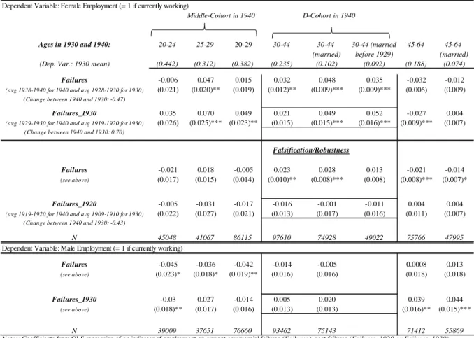
The results are reported in Table 2. In response to improving current economic conditions, all women in the D-cohort worked less. However, economic conditions dating back to the onset of the Great Depression had a lasting impact on the current work propensity of only married women. This is also true when we isolate women in this cohort in 1940 that got married before the onset of the crisis in 1929 (relative to women of the same age in 1930 that got married symmetrically before 1919). The timing of their marriage could not have been affected by the timing of the Great Depression and their marriage likely preceded their entry in the market. This is consistent with the 1929 Crash inducing an added worker effect, whereby married women, previously not working, had to enter the market and make up for the loss in family income. Evidently, their initial entry was not a temporary adjustment to extreme events, but entailed a more substantial change in their work behavior, which effects were still present a decade later in 1940. These effects are also quantitatively important. The share of women 30 to 44 years old working was 15.75 in 1940 and 10.22 in 1930, an increase of 0.055. Hence, the higher rate of failures at the onset of the Great Depression explains 62.3% of this increase (0.623=0.049*0.70/0.055). Interestingly, older women did not display employment patterns similar to the D-cohort. On the other hand, much younger women also worked more where the downturn was more severe. Nevertheless, as will be shown subsequently and in contrast to the D-cohort, the link between the labor supply and the Great Depression for these younger women will not persist in future decades.
Next, we estimate equation (1) including average commercial failures in the early 1920s instead of failures during the Great Depression.9 As can be seen the estimates are not significant, confirming that our findings are unique to the Great Depression. Finally, in the last section of Table 2, we present estimates of (1) for men. We find no significant link between past economic conditions and the work behavior of men in the D-cohort. 10
Finally, in Appendix Table A1 we provide a similar analysis using the 1920-1930 panels. As the employment status is not available in the 1920 Census, we use as dependent
8 These are averages over the last 3 years: 1938 through 1940 for 1940 and 1928 through 1930 for 1930.
9 For the exercise presented in the second section of Table 2, instead of a 10-year, we use a 20-year lag in failures. We allow for 1940 (1930) work to be affected by average economic conditions from 1919 to 1920 (1909 to 1910 for 1930).
10 Men 45 to 64 years old also increased participation in states more affected by the Great Depression. We find, however, that these effects do not extend to later decades.
13
Table 2: Employment & Commercial Failures 1930-1940
Dependent Variable: Female Employment (= 1 if currently working)
Middle-Cohort in 1940
Ages in 1930 and 1940: 20-24 25-29 20-29 30-44 30-44 30-44 (married 45-64 45-64
(married) before 1929) (married) (Dep. Var.: 1930 mean) (0.442) (0.312) (0.382) (0.235) (0.102) (0.092) (0.188) (0.074)
Failures -0.006 0.047 0.015 0.032 0.048 0.035 -0.032 -0.012
(avg 1938-1940 for 1940 and avg 1928-1930 for 1930) (0.021) (0.020)** (0.019) (0.012)** (0.009)*** (0.009)*** (0.006) (0.009)
(Change between 1940 and 1930: -0.47)
Failures_1930 0.035 0.070 0.049 0.021 0.049 0.052 -0.027 0.004
(avg 1929-1930 for 1940 and avg 1919-1920 for 1930) (0.026) (0.025)*** (0.023)** (0.015) (0.015)*** (0.016)*** (0.009)*** (0.007)
(Change between 1940 and 1930: 0.70)
Falsification/Robustness
Failures -0.021 0.018 -0.005 0.023 0.028 0.013 -0.021 -0.014
(see above) (0.017) (0.015) (0.014) (0.010)** (0.008)*** (0.008) (0.008)*** (0.007)*
Failures_1920 -0.005 -0.031 -0.017 -0.016 -0.001 -0.011 0.004 0.004
(avg 1919-1920 for 1940 and avg 1909-1910 for 1930) (0.022) (0.027) (0.021) (0.013) (0.017) (0.016) (0.011) (0.007)
(Change between 1940 and 1930: -0.43)
N 45048 41067 86115 97610 74928 49022 75766 47995
Dependent Variable: Male Employment (= 1 if currently working)
Failures -0.045 -0.036 -0.042 -0.014 -0.005 0.0008 0.013
(see above) (0.023)* (0.018)* (0.019)** (0.016) (0.016) (0.018) (0.018)
Failures_1930 -0.03 0.027 -0.014 0.005 0.020 0.039 0.044
(see above) (0.018)** (0.017) (0.016) (0.013) (0.013) (0.016)** (0.015)***
N 39009 37651 76660 93462 75143 71412 55869
Notes : Coefficients from OLS regression of an indicator of employment on current commercial failures (Failures ), past failures (Failures_1920 or Failures_1930),
age, current/birth state and year fixed effects. Sample includes white, non-farm men and women born in the United States. Failures, Failures_1930, Failures_1920 are constructed symmetrically: Failures is a vector with average failures between 1938 and 1940, for 1940 and average failures between 1928 and 1930, for 1930;
Failures_1930: average failures between 1929 and 1930, for 1940 and average failures between 1919 and 1920, for 1930; Failures_1920: average failures between
1919 and 1920, for 1940 and average failures between 1909 and 1910, for 1930. Married women in 1940 whose marriage occurred prior to 1929 are compared to married women in 1930 of the same age whose marriage occurred symmetrically before 1919. The year of first marriage can only be calculated for women. Standard errors (parentheses) are clustered by state-year. ***. **. * indicate significance at 1%. 5% and 10%
D-Cohort in 1940
variable an indicator for whether the individual reports having a gainful occupation. This analysis, therefore, is not strictly comparable to the previous one. Despite this, we obtain qualitatively similar results: the Great Depression drew into the labor market young married women from the D-cohort. The consistency of the employment patterns for the particular cohort in both panels and in relation only to the Great Depression further confirms the robustness of the findings obtained so far.
3.2. Great Depression, Economic Conditions and Female Labor Supply: 1940-1950, 1940-1960
In this section we pool data from the 1940 and 1950 and the 1940 and 1960 censuses to examine the long-term effects of the Great Depression on labor supply. We estimate equations of the following general form:
its t s ia s d k -st ts s o
its Mobrate Failures Failures 1930 Z f g
y =a +a1 +a2 +a3 _ +a4 1940, +ϕ + + +e (3)
yits is an indicator for whether a woman i in state s is employed at time t (t=1940, 1950 or 1940, 1960). In a second set of regressions we use as dependent variable the log of real
14
weekly wages. Equation (3) is a slightly modified version of (2) augmented with controls for WWII and 1940 covariates. Following Acemoglu et al. (2004) and Goldin and Olivetti (2013), we measure the labor supply effects of WWII using the share of registered men 18-44 years old who were drafted or enlisted in the war in a given state (Mobrate). We further control for the 1940 state share of men who were farmers, non-white, and for the average male education in 1940 (vector Z1940). These regressors have been shown to be significant
determinants of mobilization rates across states (Acemoglu et al., 2004). All state covariates as well as individual age and its square (vector ϕia) are interacted with a year dummy to allow for the effects of these controls to vary over time. fs and gt are state of residence/birth and year fixed effects. As before, we restrict our analysis to white non-farm men and women born in the US and not residing in group quarters.
To control for changes in current economic conditions we include Failurests, while to
capture the potentially lasting impact of the Great Depression we include as regressor k-year lagged failures (Failures_1930dst-k). Again, we construct these variables symmetrically. For
contemporary failures (Failures) we use the average failure rate over the previous three years: 1938 through 1940 if t=1940, 1948 through 1950 if t=1950 in the 1940-1950 panel, and 1958 through 1960 if t=1960 in the 1940-1960 panel. For failures during the Great Depression (Failures_1930dst-k) we use average failures from 1920 to 1923 if t=1940 and from 1930 to
1933 (core depression years) if t=1950 in the 1940-1950 panel. In the 1940-1960 panel, we use average failures from 1910 to 1913 for t=1940 and from 1930 to 1933 for t=1960. This way we allow for 1940 work (or wages) to be symmetrically affected by events as far removed as the Great Depression is to 1950 (lag k=20) or to 1960 (lag k=30).11
Tables 3 and 4 report estimates of eq. (3) using the 1940-1950 and 1940-1960 cross-sections. As before, we examine the differential impact of the variables of interest on women who were in the same age bracket in 1950 (1960) and in 1940. At the top of each age bracket we report the cohorts these women belong to when they are in the indicated age bracket in 1950 (1960).
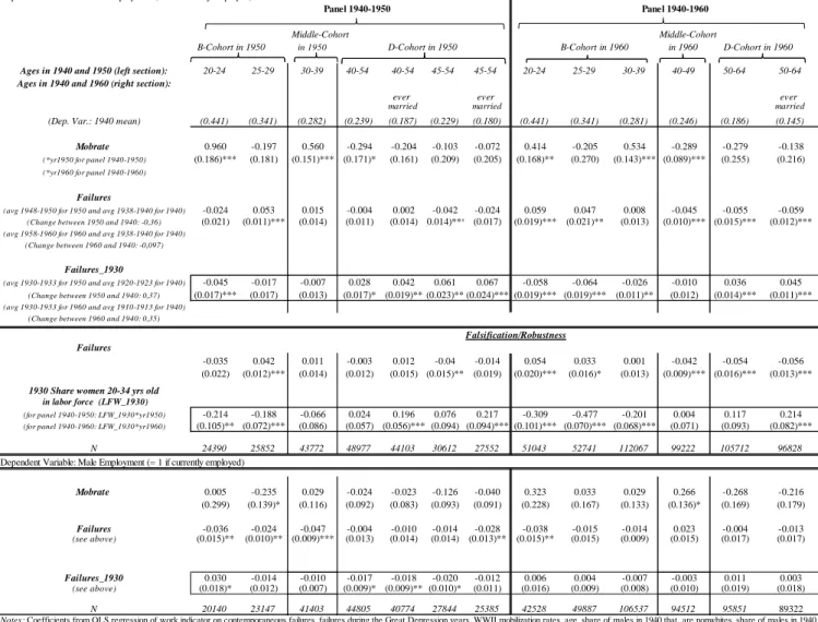
Table 3 presents results for employment. The 1940-1950 estimates show that in states with more failures during the Great Depression, 40 to 54 years old ever married women worked significantly more in 1950 than in 1940. For women 45 to 54 years old the results
11
However, 1940 itself could be affected by the Great Depression. We chose 1940 as the base year throughout because for the fertility analysis it precedes WWII and is also characterized by low births (also see Section 2 for a justification). To control for the potential impact of the Great Depression on the base year, we run specification (3) augmented by the average failures between 1930 and 1933 interacted with a 1940 year dummy. In all cases this additional regressor is not significant and the results are similar to what we report here. As a robustness check we also estimate the same regressions using the 1920-1950 and 1920-1960 panels. The results are again similar to the ones reported in the main analysis, and the effects of the Great Depression are even stronger in the 1920-1960 sample. Results are available upon request.
15
extend to all women, independently of their marital status. In contrast to the D-cohort, young women in the B-cohort (20 to 24 years old) were less likely to work in states with worse past economic conditions. The 30 to 39 year-olds, our Middle-cohort, for which we found an increased labor market presence linked to the Great Depression between 1930 and 1940, is instead not responsive to changes in economic conditions, current or past. Interestingly, women 20 to 24 years old are only affected by past but not by current conditions. This, along with the fact that these young women were not of working age during the Great Depression, suggests that the D-cohort could have crowded them out but not vice versa.
The right side of Table 3 reports estimates for the 1940-1960 panels. The most striking result is the similarity in the exit/entry pattern for young/old cohorts of women across the two panels. If anything, this pattern is stronger in 1960, as is also the link to the Great Depression. For the D-cohort, now 50 to 64 years old, this link extends to the 50 to 54 years old group for which we found no significant effects in the 1940-1950 samples (unless we focused on ever married women). Again this entry does not extend to the Middle-cohort. Instead, women in the B-cohort (20 to 39 years old), worked significantly less in states with more failures during the Great Depression. Relative to the 1940-1950 results, several cohorts also respond to improvements in contemporaneous economic conditions. These responses reinforce the impact of the Great Depression as both increase the work propensity of the D-cohort while they decrease it for women in the B-cohort.12
Regarding the impact of WWII, the estimates do not support the hypothesis that the latter led to a crowding-out of young cohorts. This would imply a decrease in their share working, while in both panels, 20 to 24 and 30 to 39 years old women were more likely to work in states with higher mobilization. Also, in both panels we find no significant link between the increased presence of the D-cohort in the labor market in the 1940s or 1950s and WWII mobilization.13
In the lower panel of the table we estimate eq. (3) but instead of commercial failures during the Great Depression, we use the state share of women in the D-cohort in the labor force in 1930 interacted with a year dummy. If the work response of the B-cohort to the Great Depression is due to the labor market behavior of the D-cohort, we would expect its
12
In an unreported analysis but available upon request we studied what the patterns documented in Table 3 imply in terms of occupations. Simple summary statistics suggest that the D-cohort occupied both blue-collar and white-collar jobs at all times and at proportions that remain remarkably stable over time (roughly 30% in blue-collar (operatives & services) and 50% in white-collar (professional/managerial & clerical) jobs. Among the white-collar occupations, 40% of these women were present in clerical jobs. Using a multinomial logit to model the presence of women across occupations, and where “out of the labor force” is our excluded category, we find that this opposite exit/entry pattern is observed most strongly in operatives as well as in clerical jobs. We also find similar patterns in professional/managerial jobs and services.
13 In Appendix Table A2, we examine the sensitivity of our estimates of interest, including the estimate of “mobrate”, in the 1940-1960 panels to different model specifications (addition/omission of covariates) and sample considerations (women of all nativities, races, farm statuses).
16
employment share in 1930 to produce effects similar to the "Failures_1930" variable in the baseline regression. The results corroborate our hypothesis: the higher the share of the
D-cohort working in 1930, the higher the share of these same women working in 1950 (1960)
and the lower the share of the B-cohort working in 1950 (1960). There are instead no effects for the Middle-cohort, which is also what we found with Failures_1930. The similarity of the results by cohort across the two panels is remarkable: they indicate a robust and persistent response pattern that is cohort-specific, still significant three decades after the 1929 Crash.
At the bottom of Table 3 we report results for men. In 1950, men in the D-cohort tend to work less in states where the Great Depression was more severe. This is consistent with an
added worker effect interpretation or possibly with older women crowding-out older men in
the labor market. While it is possible that women in the D-cohort who entered during the Great Depression acquired experience and work attachment that led them to also crowd-out men in the D-cohort, these effects are not as important as the ones found for young women and do not persist till 1960. Young men instead have a higher work propensity in states with improving contemporaneous economic conditions, which is consistent with them having the prerequisite for marriage and family life at an earlier age than men in the previous decade.
In the Appendix (Table A4) we present additional robustness checks for the 1940-1960 panels. First, we examine the impact of pre-1929 Crash conditions (Failures_1920) and find significant effects only in relation to conditions that date back to the Great Depression. Second, instead of the participation of women in the D-cohort in 1930, we use the participation of men in the same age bracket in 1930. Similarly, we find no significant effects.
Next, we turn our attention to wages. The entry/exit work patterns we have documented could be consistent with a demand and/or supply shift. Exploring the link between past conditions and contemporaneous wages could allow us to gain more insight about the nature of this shift. Table 4 reports results from the estimation of specification (3) for the 1940-1950 and 1940-1960 samples, when the dependent variable is the log of real weekly wages.14 We present estimates produced using the Heckman two-step procedure in Appendix Table A3. The latter will account for possible selection of women in the labor force. Our exclusion restriction is the number of own children present in the household.
The estimates convey three main messages. First, the most striking observation is the negative and significant estimate associated with failures in the 1930s for nearly all women in 1950 and 1960. When we use the share of women in the D-cohort working in 1930 interacted
14 The censuses prior to 1940 do not report wages and therefore a similar analysis for these years is not feasible. We restrict attention to respondents who worked more than 26 weeks in the previous year in order to obtain a sample of individuals that display some level of attachment to the labor market. Our results, however, go through even in the absence of this restriction (see Table A3).
17
Table 3: Employment 1940-1950 and 1940-1960
Dependent Variable: Female Employment (= 1 if currently employed)
Middle-Cohort Middle-Cohort B-Cohort in 1950 D-Cohort in 1950in 1950 B-Cohort in 1960 in 1960 D-Cohort in 1960
Ages in 1940 and 1950 (left section): 20-24 25-29 30-39 40-54 40-54 45-54 45-54 20-24 25-29 30-39 40-49 50-64 50-64 Ages in 1940 and 1960 (right section):
ever ever ever
married married married
(Dep. Var.: 1940 mean) (0.441) (0.341) (0.282) (0.239) (0.187) (0.229) (0.180) (0.441) (0.341) (0.281) (0.246) (0.186) (0.145) Mobrate 0.960 -0.197 0.560 -0.294 -0.204 -0.103 -0.072 0.414 -0.205 0.534 -0.289 -0.279 -0.138 (*yr1950 for panel 1940-1950) (0.186)*** (0.181) (0.151)*** (0.171)* (0.161) (0.209) (0.205) (0.168)** (0.270) (0.143)*** (0.089)*** (0.255) (0.216) (*yr1960 for panel 1940-1960)
Failures
(avg 1948-1950 for 1950 and avg 1938-1940 for 1940) -0.024 0.053 0.015 -0.004 0.002 -0.042 -0.024 0.059 0.047 0.008 -0.045 -0.055 -0.059 (Change between 1950 and 1940: -0,36) (0.021) (0.011)*** (0.014) (0.011) (0.014) (0.014)*** (0.017) (0.019)*** (0.021)** (0.013) (0.010)*** (0.015)*** (0.012)*** (avg 1958-1960 for 1960 and avg 1938-1940 for 1940)
(Change between 1960 and 1940: -0,097)
Failures_1930
(avg 1930-1933 for 1950 and avg 1920-1923 for 1940) -0.045 -0.017 -0.007 0.028 0.042 0.061 0.067 -0.058 -0.064 -0.026 -0.010 0.036 0.045 (Change between 1950 and 1940: 0,37) (0.017)*** (0.017) (0.013) (0.017)* (0.019)** (0.023)** (0.024)*** (0.019)*** (0.019)*** (0.011)** (0.012) (0.014)*** (0.011)*** (avg 1930-1933 for 1960 and avg 1910-1913 for 1940)
(Change between 1960 and 1940: 0,35)
Falsification/Robustness Failures
-0.035 0.042 0.011 -0.003 0.012 -0.04 -0.014 0.054 0.033 0.001 -0.042 -0.054 -0.056 (0.022) (0.012)*** (0.014) (0.012) (0.015) (0.015)** (0.019) (0.020)*** (0.016)* (0.013) (0.009)*** (0.016)*** (0.013)***
1930 Share women 20-34 yrs old in labor force (LFW_1930)
(for panel 1940-1950: LFW_1930*yr1950) -0.214 -0.188 -0.066 0.024 0.196 0.076 0.217 -0.309 -0.477 -0.201 0.004 0.117 0.214 (for panel 1940-1960: LFW_1930*yr1960) (0.105)** (0.072)*** (0.086) (0.057) (0.056)*** (0.094) (0.094)*** (0.101)*** (0.070)*** (0.068)*** (0.071) (0.093) (0.082)***
N 24390 25852 43772 48977 44103 30612 27552 51043 52741 112067 99222 105712 96828 Dependent Variable: Male Employment (= 1 if currently employed)
Mobrate 0.005 -0.235 0.029 -0.024 -0.023 -0.126 -0.040 0.323 0.033 0.029 0.266 -0.268 -0.216 (0.299) (0.139)* (0.116) (0.092) (0.083) (0.093) (0.091) (0.228) (0.167) (0.133) (0.136)* (0.169) (0.179) Failures -0.036 -0.024 -0.047 -0.004 -0.010 -0.014 -0.028 -0.038 -0.015 -0.014 0.023 -0.004 -0.013 (see above) (0.015)** (0.010)** (0.009)*** (0.013) (0.014) (0.014) (0.013)** (0.015)** (0.015) (0.009) (0.015) (0.017) (0.017) Failures_1930 0.030 -0.014 -0.010 -0.017 -0.018 -0.020 -0.012 0.006 0.004 -0.007 -0.003 0.011 0.003 (see above) (0.018)* (0.012) (0.007) (0.009)* (0.009)** (0.010)* (0.011) (0.016) (0.009) (0.008) (0.010) (0.019) (0.018) N 20140 23147 41403 44805 40774 27844 25385 42528 49887 106537 94512 95851 89322 Notes : Coefficients from OLS regression of work indicator on contemporaneous failures, failures during the Great Depression years, WWII mobilization rates, age, share of males in 1940 that are nonwhites, share of males in 1940 that are farmers, 1940 average male education, state of birth, sate of residence and year fixed effects. Sample includes white, non-farm men and women born in the United States. Failures, Failures_1930 and Failures_1920 are constructed symmetrically: Failures are contemporanous failures: for the panel 1940-1950, we use the average between 1938 and 1940 for the year 1940 and the average between 1948 and 1950 for 1950, for the panel 1940-1960 we use average failures between 1938 and 1940 for 1940 and average failures between 1958 and 1960 for 1960. The change in Failures between 1950 and 1940 is -0.36, between 1960 and 1940, -0.097. Failures_1930 are failures during the Great Depression: for the panel 1940-1950, we use average failures between 1920-1923 for 1940 and average failures between 1930-1933 for 1950; for the panel 1940-1960, we use average failures between 1910 and 1913 for 1940 and average failures between 1930 and 1933 for 1960. The change in Failures_1930 between 1950 and 1940 is 0.37, between 1960 and 1940, 0.035. Standard errors (parentheses) are clustered by state-year. ***, **, * indicate significance at 1%, 5% and 10% respectively. Sources: 1940-1950 and 1940-1960 IPUMS USA, Statistical Abstracts of the United States.
Panel 1940-1950 Panel 1940-1960
with a year dummy, we find similar results. These results are consistent with the hypothesis that the channel via which the Great Depression decreased female wages was an outward shift in the labor supply of women in the D-cohort.
Improvements in current economic conditions either do not significantly affect older cohorts, or decrease their wages in 1950. This suggests that the entry of the D-cohort in the labor market was not due to a labor demand shift driven by contemporaneous labor market shortages. If the labor demand for older women had shifted out to compensate for the exit of the younger that choose to form families, in a reverse causality sense, we would have expected some upward pressure on their wages in relation to changes in current economic conditions.
Second, in 1950 the wages of 20 to 24 years old women were subject to two opposite forces: a decrease due to conditions in the early 1930s and an increase due to the current
18
economic boom. However, the quantitative impact of the Great Depression on their wages was more than twice as important as that due to improving current conditions. In 1960, the positive impact of current conditions becomes more relevant; possibly starting to reflect the effect of the retirement of the older cohort on labor markets.15
Third, the Heckman-corrected estimates further confirm that the uniformly negative effect of past conditions on current wages is not due to selection. Such a selection would occur if, for instance, the Great Depression drew in the labor market women with “worse” unobservable characteristics, possibly employed in lower-skill, more “brawn”-type occupations. In response, women with “better” unobservable characteristics would drop-out of the workforce. This selection mechanism could manifest as a decrease in women’s wages, conditional on their observable characteristics. Thus, the changing composition in the female workforce linked to the Great Depression could in part or entirely explain our finding of lower wages decades after the 1929 Crash in the OLS regressions. Our results show, however, that, although there has been negative selection in the workforce across all cohorts of women entering in 1950 and 1960, this selection neither significantly alters our previous findings of a persistent wage decline linked to the Great Depression nor contradicts our interpretation of a labor supply shift. In fact, the adjusted estimates suggest an even stronger effect of the Depression in lowering contemporaneous wages for women in all age groups. Our findings are consistent with Mulligan and Rubinstein (2008), who also uncover a negative selection in the female workforce in the 1970s and a reversal later on in the 1980s. Our findings suggest that this negative selection predated the 1970s.
To summarize, we have presented a series of newly documented facts that highlight the pervasive role of the Great Depression on labor markets. This event drew into the workforce young married women, 20 to 34 years old at the time of the 1929 Crash (D-cohort), likely via an added worker effect. Their entry, persistently linked to the Depression and reinforced by the subsequent economic boom, was remarkably sustained in the 1940s and 1950s. It also led to a decline in the wages of all women, including the very young. We interpret these findings as supportive of a labor supply shift for the D-cohort that crowded-out younger women. The entry of the D-cohort is not surprising given the age of these women at the time of the Crash. Their husbands may have been unemployed for long periods in the 1930s and their salary may have suffered permanently; they may have lost homes with mortgages, businesses or savings. Sufficiently large wealth and income losses could have
15
19 permanently shifted out labor supply.16
Table 4: Wages: 1940-1950 and 1940-1960 (Dep. Variable: Log real weekly wage)
Dependent Variable: Female Wages
Panel 1940-1950 Panel 1940-1960
Middle- Middle- D-Cohort
B-Cohort in 1950 Cohort in 1950 D-Cohort in 1950 B-Cohort in 1960 Cohort in 1960 in 1960
Ages in 1940 and 1950 (left section): 20-24 25-29 30-39 40-54 45-54 20-24 25-29 30-39 40-49 50-64
Ages in 1940 and 1960 (right section):
Mobrate -0.644 -0.683 0.386 -0.690 0.337 -1.152 -0.467 -0.968 -1.718 -1.351 (0.421) (0.426) (0.367) (0.553) (0.883) (0.353)*** (0.391) (0.326)*** (0.662)** (0.819) Failures -0.099 0.074 -0.009 0.025 0.005 -0.171 -0.054 -0.025 -0.004 0.101 (see Table 3) (0.033)*** (0.026)*** (0.039) (0.031)** (0.055) (0.045)*** (0.037) (0.043) (0.050) (0.091) Failures_1930 -0.196 -0.110 -0.063 -0.140 -0.197 -0.063 -0.082 -0.075 -0.183 -0.072 (see Table 3) (0.038)*** (0.037)*** (0.035)* (0.050)*** (0.067)*** (0.036)* (0.042)* (0.027)*** (0.057)*** (0.081) Failures -0.122 0.081 -0.042 -0.026 -0.047 -0.165 -0.039 -0.037 -0.061 0.029 (see Table 3) (0.036)*** (0.034)** (0.039) (0.033) (0.048) (0.049)*** (0.041) (0.046) (0.054) (0.100)
1930 Share women 20-34 yrs old -0.523 -0.021 -0.554 -0.953 -1.005 -0.102 -0.054 -0.421 -1.384 -1.280
in labor force (LFW_1930) (0.172)*** (0.178) (0.198)*** (0.273)*** (0.383)** (0.187) (0.213) (0.231)* (0.255)*** (0.347)*** (see Table 3)
N 8956 7268 11172 12148 7297 19320 14766 30888 33819 31325
Notes: Dependent variable: log weekly wages. Worked more than 26 weeks in previous year. For details see footnote to Table 3.
4. A Measure of Crowding-Out and Crowding-In
As Figure 1 shows, in no other previous decades had so many older women been part of the workforce as in the 1940s and 1950s. Relative to the past, there is a sharp change between 1940 and the later years. Our analysis traces the entry of these women back to the Great Depression and the subsequent economic recovery. No employment link is found to WWII. While these effects were confined to married women in this cohort until 1940, they became pervasive in the later decades.
To assess the impact of the work behavior of the D-cohort on yearly and completed fertility, we proceed in three steps. First, we construct state measures that summarize our crowding-out/crowding-in hypothesis as a function of the life-cycle labor supply changes of the D-cohort. Second, we show that these measures can successfully predict the employment behavior of women in the B-cohort: relative to 1940 they work significantly less in 1960 and more in 1970. Third, we show that the same measures can predict a baby-boom in the 1950s and later on a baby-bust for the B-cohort. In line with the analysis of Section 3, our reference point for births also remains their level in 1940.
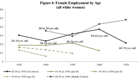
To motivate our first step, we provide a visual representation of the life cycle labor supply profile of the D-cohort. We also contrast it to the profiles of other contiguous cohorts,
16 In separate work that is currently in progress, we examine plausible channels through which the Great Depression led to the persistent increase in the work propensity of the D-cohort in 1950 and 1960.
20 20 to 29 yrs old 0 0,1 0,2 0,3 0,4 0,5 0,6 1930 1940 1950 1960 1970
Figure 4: Female Employment by Age (all white women)
20-34 in 1930 (D-cohort) 35-44 in 1930 (pre-D) 45-54 in 1930 (pre-D) 55-64 in 1930 (pre-D) 20-29 in 1940 (Middle Cohort)
20-34 yrs old
30-44 yrs old 40-54 yrs old
50-64 yrs old 60-74 yrs old 20 to 29 yrs old 0 0,05 0,1 0,15 0,2 0,25 0,3 0,35 0,4 0,45 1930 1940 1950 1960 1970
Figure 5: Female Employment by Age (white married women)
20-34 yrs old 30-44 yrs old 40-54 yrs old 50-64 yrs old 60-74 yrs old 0 0,1 0,2 0,3 0,4 0,5 0,6 1960 1962 1963 1964 1965 1966 1967 1968 1969 1970 age in 1960: 50-54 age in 1960: 55-59 age in 1960: 60-64 age in 1960: 45-49
Figure 6: Employment Shares of the D-Cohort in the 1960s (CPS)
three older and one younger. These are summarized in Figures 4 (all women) and 5 (married). Between 1930 and 1940, overall fewer women in the D-cohort worked, while married women worked more in the spirit of the added worker effect. The year 1940 marks the beginning of their increased aggregate presence in the market, as all work more regardless of their marital status. Interestingly, the time-frame of the entry/exit of the D-cohort is the mirror image of the baby-boom/ bust.
21
Figures 1 and 4 also illustrate two other important trends, on the basis of which we construct our measures. First, between 1930 and 1940, there is essentially only one cohort significantly exiting the labor market and hence freeing up positions for the new entrants. These are women 30 to 44 years old in 1940 (20 to 34 years old in 1930), our D-cohort. The labor market presence of older women remains instead roughly the same between 1930 and 1940 as older cohorts did not significantly re-enter the labor market after having had children. This means that the behavior of the D-cohort when young adequately describes the most important changes in the labor market in the 1930s. Second, in later decades this same
D-cohort, when older, instead re-enters the workforce filling up positions and likely limiting
opportunities for the new entrants.17 This suggests that the entire life-cycle labor supply of the
D-cohort has the potential to affect work and fertility decisions of younger women over a
period of several decades.
Our next task is to construct CO and CI measures reflecting these observations. Young entrants’ perception of their market options comes from observing wages and other labor market indicators. The entry of the D-cohort in the 1940s and 1950s decreased wages and market opportunities for young women entering the workforce in the 1950s. In absence of data on wages prior to 1940 or other annual indicators of labor market tightness, we use state-level changes across decades in the share of women in the D-cohort working to predict the market exit/entry of the younger cohorts.18 To predict the work (and births) of the B-cohort in the 1950s we use the change in the share of women in the D-cohort working between 1950 and 1940: / / 44 30 1940 , , 44 30 1940 , , 54 40 1950 , , 54 40 1950 , , 1950
∑
∑
∑
∑
= = = = = i i s i i s i i s i is pop work pop
work CO
An increase in CO means that there were more women working in 1950 than in 1940. The largerCO1950, the bigger the increase in the share of women in the D-cohort entering in
the1940s, the lower the wages and the fewer the labor market opportunities for the younger potential entrants.
To capture the impact of the retirement of the D-cohort we adopt a similar strategy and use the change in its work shares between 1960 and 1970:
17 Aside from the D-cohort, women 30-39 years old in 1950 also enter the market in the 1950s. As discussed, however, in the robustness analysis of Section 5 (estimates presented in the Appendix), the impact of the D-cohort on fertility remains unaffected when considering the entry/exit into/from the market of other cohorts.
18 In a two-period world, with both young (Ny
t) and old women (Not) in the workforce, young women entering into the labor market are not directly competing with the older who entered in the previous period (No
t-1), as the latter have more experience. Rather they compete more closely with older women who are entering for the first time or re-entering after a long absence (No
t - Not-1). Using the change over a decade in the share of older women working (No
t - Not-1 = older new entrants) rather than the share of all older women working (Not),which also includes Not-1, captures this idea.
22 / / 74 60 1970 , 74 60 1970 , 64 50 1960 , 64 50 1960 , 1970
∑
∑
∑
∑
= = = = = − i i i i i i ii pop work pop
work CI
As the D-cohort retires, we expect its work share in 1970 to decline and the CI measure to increase. The higher its retirement, the more work opportunities should arise for younger women and the higher the likelihood that they will enter the market thus reducing births. Figure 6 provides a more detailed description of the retirement process of the D-cohort using annual micro data on employment from the Current Population Survey (March CPS).19 Within the D-cohort we distinguish three groups. The oldest will likely retire in the early part of the 1960s, the youngest in the later part. The figure indeed shows a significant decline in the work shares of the oldest cohorts in the early 1960s, when we start to observe a reversal of the baby-boom. We also report the work shares of younger women, 45 to 49 years old in 1960, who as can be seen do not retire in the 1960s.
Finally, to predict the work patterns (and births) of the B-cohort in 1940 we use the change in the share of the D-cohort working between 1940 and 1930:
/ -/ 34 20 1930 , , 34 20 1930 , , 44 30 1940 , , 44 30 1940 , , 1940
∑
∑
∑
∑
= = = = = i i s i i s i i s i is pop work pop
work CO
There is a slight asymmetry between the CI1970 and the CO1950 measures. The CO1950 uses
changing work shares between 1940 and 1950 to predict crowding-out and births in each year in the 1950s, while the CI1970 uses actual retirement occurring between 1960 and 1970. The CO1950
allows a separation between the (past) entry of the D-cohort and the (future) births of the B-cohort, which should reduce the possibility of reverse causality or simultaneity between the decision of the old and of the young. A simultaneity issue would arise if we were to use as our measure the change in the 1950-1960 work shares of the D-cohort, the period when the baby-boom is observed. On the other hand, between 1950 and 1960, the D-cohort kept entering into the labor market (Figures 4 and 5). This entry cannot predict their retirement a decade later. For this reason, we need to use the change in their employment between 1960 and 1970, over which period most of the D-cohort actually retired. Since retirement decisions are mostly driven by age, we feel that there is less of an endogeneity issue, or possible reverse causality, in approximating their retirement with the change in their work shares between 1960 and 1970.
Before using these measures to assess their impact on births, we examine if they can predict changes in the share of the B-cohort working between 1940-1960 and 1940-1970. This
19
23
is the channel via which we hypothesize that the D-cohort should affect the fertility of women in the B-cohort. For the panels 1940-1960, we estimate:
) 4 ( , 1940 5 st 3 1 s s ia s t its o its Mobrate Z f g y =b +b +bCO +b +ϕ + + +e
For the panels 1940-1970, we instead include the crowding-in measure:
) 5 ( , 1940 5 st 3 1 s s ia s t its o its Mobrate Z f g y = b +b +bCI +b +ϕ + + +e
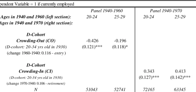
The dependent variable is 1 if a woman is currently working. CO and CI are our measures of crowding-out and crowding-in respectively.20 The other variables have been defined previously. We don’t include CO and CI in the same regression because they will be highly correlated as they summarize the behavior of the same cohort at different points in time. The estimates presented in Table 5 show that the entry of the D-cohort into the labor market between 1940 and 1950 predicts a decrease in the share of young women working in 1960. Between 1940 and 1970, instead, the crowding-in term induces the opposite effect: as the
D-cohort exits, significantly more young women enter the labor market. Therefore, the measures
devised capture the labor market changes we have hypothesized.
Table 5: Crowding-Out, Crowding-In & Labor Supply of Young Women (1940-1960, 1940-1970) Dependent Variable = 1 if currently employed
Ages in 1940 and 1960 (left section): 20-24 25-29 20-24 25-29
Ages in 1940 and 1970 (right section): D-Cohort
Crowding-Out (CO) -0.426 -0.196
(D-cohort: 20-34 yrs old in 1930) (0.121)*** (0.118)* (change 1960-1940: 0.116 - entry )
D-Cohort
Crowding-In (CI) 0.343 0.413
(D-cohort: 20-34 yrs old in 1930) (0.127)*** (0.142)***
(change 1970-1940: 0.106 - retirement)
N 51043 52741 72165 63345
Notes: Coefficients from OLS regression of work indicator on WWII mobilization rates, age, share of males in 1940 that are nonwhites, share of males in 1940 that are farmers, 1940 average male education, state and year fixed effects. Sample includes white, non-farm women born in the United States. Standard errors (parentheses) clustered by state-year. ***, **, * indicate significance at 1%, 5% and 10% respectively.
Panel 1940-1960 Panel 1940-1970
As a final related remark, Figure 4 shows there are few cohorts which could rival or diminish the impact of the D-cohort. The Middle-cohort is evidently the most important, but
20