Science Arts & Métiers (SAM)
is an open access repository that collects the work of Arts et Métiers Institute of
Technology researchers and makes it freely available over the web where possible.
This is an author-deposited version published in: https://sam.ensam.eu Handle ID: .http://hdl.handle.net/10985/9177
To cite this version :
Benjamin LAMOUREUX, Jean-Rémi MASSÉ, Nazih MECHBAL - Diagnostics of an Aircraft Engine Pumping Unit Using a Hybrid Approach based-on Surrogate Modeling - In: IEEE Conference on Prognostics and Health Management, United States, 2013 IEEE PHM 2013 -2013
Any correspondence concerning this service should be sent to the repository Administrator : [email protected]
Diagnostics of an Aircraft Engine Pumping Unit
Using a Hybrid Approach based-on Surrogate
Modeling
Benjamin Lamoureux, Jean-Rémi Massé
R&D department – Regulation Systems Division Safran Snecma
Moissy-Cramayel, France [email protected]
Nazih Mechbal
DYSCO – Dynamic of Structures, Systems and Control Arts et Métiers ParisTech - PIMM UMR 8006
Paris, France [email protected] Abstract—This document introduces a hybrid approach for fault
detection and identification of an aircraft engine pumping unit. It is based on the complementarity between a model-based approach accounting for uncertainties aimed at quantifying the degradation modes signatures and a data-driven approach aimed at recalibrating the healthy syndrome from measures. Because of the computational time costs of uncertainties propagation into the physics based model, a surrogate modeling technic called Kriging associated to Latin hypercube sampling is utilized. The hybrid approach is tested on a pumping unit of an aircraft engine and shows good results for computing the degradation modes signatures and performing their detection and identification.
Keywords-Prognostics and Health Management, hybrid approach, detection, identification, degradations, surrogate modeling, kriging, Latin hypercube sampling
I. INTRODUCTION
In recent years, availability was raised to the status of strategic challenge for many industries mainly because a great amount of the average costs is attributable to Maintenance, Repair and Overhaul (MRO) and Delays and Cancellations (D&C). For example, in aeronautics, they represent a quarter of the total expenses for airliners. In order to optimize availability, novel MRO strategies are under development, based on failure anticipation and real-time optimization of maintenance plan. Most of them are issued from Prognostics and Health Management (PHM), and the most proven one is Conditioned Based Maintenance (CBM) [1].
Typically, PHM is either model-based [2] or data-driven [3] but unfortunately, both of these methods have their limitations. On the one hand, instead of its good precision in degradation modeling and sensitivity analysis, model-based approaches have some difficulties adapting to environmental variations and unclassifiable, but significant, perturbations. On the other hand, data-driven approaches are suitable ways to take into account uncertainties but they show their limit when confronted to the problem of lack of available measured data. Actually, this problem is dual: First, measured data are needed in the upstream development stages in order to perform the learning step of data-driven algorithms but in practice they are
not available before the entry into service, which is too late if the system suffers from prohibitive controller retrofit costs. Then, measured data of degraded states are needed for creating a degradation signature database but if the system has a good reliability, these data are not numerous enough to manage the stochastic nature of PHM.
As both approaches have their weaknesses, it is interesting to combine them in a hybrid approach. This kind of approach is quite uncommon in the scientific community, but it has already been applied. For example, Garga et al. [4] have described a hybrid reasoning approach that integrates domain knowledge with test and operational data from an industrial gearbox and Kumar et al. [5] have proposed a hybrid prognostics framework aimed at performing the PHM of electronic products. In this paper, a hybrid approach is also used. It combines the advantages of following approaches: the model-based one to quantify the degradation modes signatures and their related damage model in upstream development stages and the data-driven one to recalibrate the healthy syndrome in downstream stage.
The remainder of the document is organized as following: In the next section, the hybrid approach is introduced. The second section addresses surrogate modeling and particularly Kriging and section IV and V are dedicated to an application on a pumping unit of an aircraft engine.
II. HYBRID APPROACH
In this section, the monitoring of a system 𝒮 using a hybrid approach is addressed. Its deterministic numerical model is 𝒻 so that:
(𝜂1, … , 𝜂ℎ) = 𝒻(𝑼, 𝛽1, … , 𝛽𝑝, 𝛾1, … , 𝛾𝑑) (1)
where 𝑼 ∈ ℝ𝑛×𝑘 is the matrix of the model inputs (variables
evolving with time during a run), 𝑘 is the number of samples, 𝜂1, … , 𝜂ℎ are the Health Indicators (HI) values, 𝛽1, … , 𝛽𝑝 are
the context parameters (constant during a run) and 𝛾1, … , 𝛾𝑑
are the degradation values. A degradation is defined by its mode 𝑗 (index of the degradation parameter) and its magnitude
𝜔 (value of the parameter). The nominal magnitude, or healthy magnitude of a degradation mode 𝑗 is written 𝜔0𝑗.
A. Model-Based Framework 1) Uncertainties Management
Taking into account uncertainties consists in replacing the deterministic parameters 𝛽1, … , 𝛽𝑝 by the random variables
𝜷1, … , 𝜷𝑝. They can be characterized by their probability
density functions (pdf). A pdf is completely defined by its type (uniform, normal, exponential…) and its parameter vector 𝚯. These pdf are often determined through experience feedback or expertise.
Thanks to uncertainties, it is possible to compute stochastic HI distributions from a deterministic model by randomly sampling model parameters values according to their pdf. This operation is called uncertainties propagation [6]. Many tools are available for uncertainties propagation but the most famous and proven one is the Monte-Carlo algorithm. In this case, Equ.1 can be written in its stochastic form:
(𝜼1, … , 𝜼ℎ) = 𝒻(𝑼, 𝜷1, … , 𝜷𝑝, 𝛾1, … , 𝛾𝑑) (2)
where 𝜼𝟏, … , 𝜼ℎ are random variable corresponding to the HI
distributions.
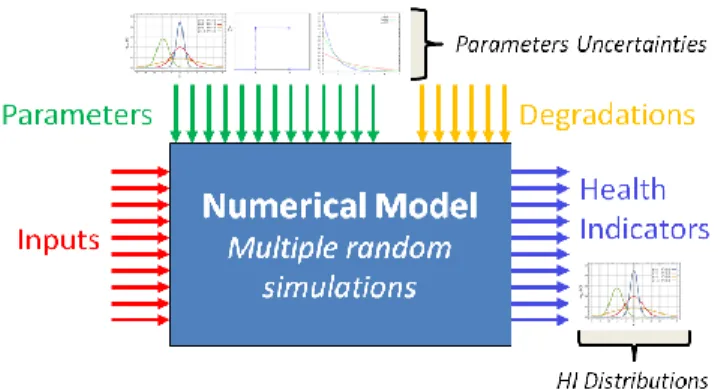
Figure 1. Model-based framework scheme 2) Simulated Health Indicators
The purpose of the model-based approach is to create simulated data to overcome the lack of measured data in upstream development stages. Simulated pdf Parameters (SP) are defined for each triplet (HI 𝑖, mode 𝑗, magnitude 𝜔) as following:
𝑺𝑷(𝑖, 𝑗, 𝜔) = ( 𝜃𝑗𝑖 1(𝜔), … , 𝜃𝑗𝑖 𝑟(𝜔)) 𝑇
(3) where 𝑟 is the number of parameters for the chosen type of pdf and 𝜃𝑗𝑖 𝑘(𝜔), 𝑘 = 1, … , 𝑟 is the value of the pdf parameters of
𝜼𝑖 obtained by Maximum Likelihood Estimation (MLE) for
𝒻(𝑼, 𝜷1, … , 𝜷𝑝, 𝜔𝛿1𝑗, … , 𝜔𝛿𝑗𝑗, … 𝜔𝛿𝑑𝑗) with 𝛿𝑘𝑙 Kronecker
delta. It can be noticed that if 𝜔is equal to 0, then the SP corresponds to the parameter vector of a healthy distribution.
3) Damage Models
Fixing the HI index 𝑖 and the degradation mode 𝑗 , it is supposed that the SP has been computed for k values
of magnitude 𝜔1, … , 𝜔𝑘. From these values, it is possible to
construct regression models for 𝑗𝑖𝜃𝑘(𝜔), 𝑘 = 1, … , 𝑟 via Least
Square Estimation (LSE) as shown in Equ.4. 𝜃
𝑗𝑖 𝑘(𝜔) = ℊ𝑘𝑇(𝜔) 𝝀𝒋𝒊 𝒌 (4)
where ℊ𝑘 are the regression functions and 𝒋𝒊𝝀𝒌 the regression
coefficients. The Damage Model of HI 𝑖 and degradation mode 𝑗 is defined as the following matrix:
𝑫 𝒋 𝒊 = | 𝝀 𝟏 𝒋 𝒊 … 𝝀 𝒓 𝒋 𝒊 | (5) Thus, 𝓰𝑇(𝜔) 𝑫 𝒋 𝒊 , 𝓰 = (ℊ 1, … , ℊ𝑟) is the LSE of 𝑺𝑷(𝑖, 𝑗, 𝜔).
4) Degradation Mode Simulated Signatures
Considering a given degradation mode 𝑗and its magnitude 𝜔 , the Simulated Syndrome (SSy) is a matrix defined as following: 𝑺𝑺𝒚(𝑗, 𝜔) = |𝓰𝑇(𝜔) 𝑫 𝒋 𝟏 … 𝓰𝑇(𝜔) 𝑫 𝒋 𝒉 |𝑇 (6)
where ℎ is the number of HI. Then, the simulated healthy syndrome (ShSy) is defined whatever the degradation mode 𝑗 as following:
𝑺𝒉𝑺𝒚 = 𝑺𝑺𝒚(𝑗, 𝜔0𝑗) (7) The Maximal Admissible Magnitude (MAM) is defined as the magnitude for which the system reaches a failure state and is written 𝜔𝑀𝐴𝑀𝑗 for degradation mode 𝑗. The Signature (Sg) of
a degradation mode 𝑗 is the difference between simulated MAM and simulated healthy syndromes. It is defined as following:
𝑺𝒈(𝑗) = 𝑺𝑺𝒚(𝑗, 𝜔𝑀𝐴𝑀𝑗 ) − 𝑺𝒉𝑺𝒚 (8)
B. Data-Driven Part
The data-driven process consists first in an extraction of real HI. Then, supposing that the data correspond to a healthy state of the system, which is normally the case just after the entry into service, a MLE of the measured HI distributions pdf parameters is performed to compute the measured healthy syndrome (MhSy) which is defined as following:
𝑴𝒉𝑺𝒚 = |𝑴𝒉𝑺𝒚𝟏 … 𝑴𝒉𝑺𝒚𝒉|𝑇 (9)
where 𝑴𝒉𝑺𝒚𝒌 = (𝜃1𝑘, … , 𝜃𝑟𝑘)𝑇, 𝑟 is the number of parameters
for the chosen type of pdf and 𝜃𝑘𝑖, 𝑘 = 1, … , 𝑟 are the MLE
values of the pdf parameters of the measured distribution of HI 𝑖. Provided both MhSy and damage model are available, it is possible to calculate the Recalibrated Syndromes (RSy) defined as following:
𝑹𝑺𝒚(𝑗, 𝜔) = 𝑺𝑺𝒚(𝑗, 𝜔) − 𝑺𝒉𝑺𝒚 + 𝑴𝒉𝑺𝒚 (10) The recalibrated failure syndrome (RfSy) is defined for a given degradation mode 𝑗 as the syndrome corresponding to the MAM:
The RfSy is particularly useful for the detection process because it is derived from the true healthy values of HI. C. Detection and Identification Performance
In order to quantify the performance of the detection and identification processes, some performance metrics called Key Performance Indicators (KPI) need to be defined.
For detection, the KPI are usually the False Positive ratio (FP) and the True Positive ratio (TP) [7] computed for the best threshold. FP is equivalent to the rate of type I error or false alarms and TP is equivalent to the rate of true alarms. The best threshold is defined as the threshold for which the couple (FP; TP) is the further from the no-discrimination line and it can be determined graphically from the analysis of Receiver Operating Characteristic (ROC) curves. An example of a ROC curve from the Matlab© dataset is given in figure 2. FP and TP are computed for each degradation mode 𝑗 between 𝑺𝒉𝑺𝒚 and 𝑹𝒇𝑺𝒚(𝑗).
Figure 2. Example of ROC curve from matlab. The grey dashed line is the no-discrimination line.
For identification, the KPI is called the Distinguishability vector, written 𝑫 = (𝐷1, … , 𝐷𝑟)𝑇, with coefficient 𝐷𝑘 defined
for two signatures as following: 𝐷𝑘(𝑖, 𝑗) = cos−1(
𝑺𝒈𝒌(𝑖)𝑻𝑺𝒈𝒌(𝑗)
‖𝑺𝒈𝒌(𝑖)‖‖𝑺𝒈𝒌(𝑗)‖) (12)
where 𝑺𝒈𝒌(𝑖) and 𝑺𝒈𝒌(𝑗) 𝑘 = 1, … , 𝑟 design the kth column
of the signature matrices. Typically, specifications require 𝑇𝑃 > 80% and 𝐹𝑃 < 5%. The vector 𝑫 is a way to quantify the angle between two signatures so in fine the potential for discrimination between degradation modes.
Finally, it is obvious that in order to compute the damage models, a huge amount of measures is needed (c.f. Equ.4.). However, if the numerical physics based model of the system is expensive in terms of computation time, it is not possible to run all the needed simulations. In the next section, a solution is introduced through surrogate modeling whose aim is basically to construct a “low cost” model of model.
III. SURROGATE MODELING AND KRIGING A. Surrogate Modeling Basics
When physics based models are expensive in terms of computation time, it is interesting to use surrogate modeling. For instance, it is used to optimize aerospace design [8]. A surrogate model is a mathematic function:
Of negligible computation cost
Approximating the physics based model responses A surrogate modeling process is composed of the following steps, also presented in figure 3:
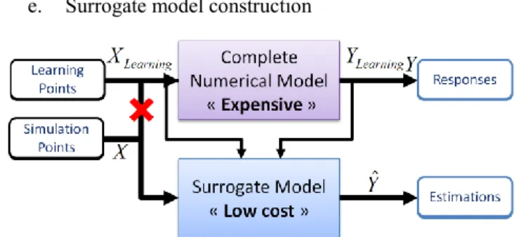
a. Determination of the variation range of influential parameters and their pdf uncertainty management b. Choice of the surrogate model type (ex: Kriging) c. Design sample construction (Design of Experiment) d. Scatter plot of the learning sample (Visual Checking) e. Surrogate model construction
Figure 3. Principle of surrogate modeling. The “low cost” model is constructed from 𝑋𝐿𝑒𝑎𝑟𝑛𝑖𝑛𝑔 and 𝑌𝐿𝑒𝑎𝑟𝑛𝑖𝑛𝑔
B. Design of Experiment
As shown in figure 3, some learning points, also called design sites, are requested in order to build a surrogate model. In order to optimize the sites selection, Design of Experiment (DOE) are constructed. Even if the type of DOE to be used depends on the surrogate model, the choice is typically made among low discrepancy DOE in order to browse in an exhaustive way the variation range of model parameters space. For instance, Latin Hypercube Sampling (LHS) is widely used with Kriging in order to create design sites from multidimensional pdf of 𝑝 variables. LHS consists in the following steps:
1. Discretization of the 𝑝 pdf into 𝑛 intervals with equal probability. Intervals are noted: ℐ1𝑝, … , ℐ𝑛𝑝.
2. Creation of a permutation matrix 𝑨 ∈ ℕ𝑛×𝑝:
𝑨 = |𝜎
1(1) ⋯ 𝜎𝑝(1)
⋮ ⋱ ⋮
𝜎1(𝑛) ⋯ 𝜎𝑝(𝑛)| (13)
where 𝜎1, … , 𝜎𝑝 are permutations of ⟦1; 𝑛⟧
3. Random sampling according to the different pdf in order to construct the DOE.
0 0.2 0.4 0.6 0.8 1 0 0.1 0.2 0.3 0.4 0.5 0.6 0.7 0.8 0.9 1
False Positive Rate
T ru e P o si tive Ra te Class 1 Class 2 Class 3 Class 4
𝑫𝑶𝑬 = |
𝑟𝑎𝑛𝑑( ℐ𝜎11(1)) ⋯ 𝑟𝑎𝑛𝑑( ℐ𝜎𝑝𝑝(1))
⋮ ⋱ ⋮
𝑟𝑎𝑛𝑑( ℐ𝜎11(𝑛)) ⋯ 𝑟𝑎𝑛𝑑( ℐ𝜎𝑝𝑝(𝑛))
| (14) where 𝑟𝑎𝑛𝑑 is a function drawing randomly a value according to an interval pdf.
The main advantage of LHS is that it can produce low discrepancy DOE not only in the global space but also in each single dimension. However, the quality of LHS DOE is not homogeneous and it can be interesting to use an optimization criterion such as in [9].
C. Kriging
Originally, Kriging was developed by the mining engineer Daniel Krige for interpolation in geostatistics before being applied to numerical modeling. See [10] for a recent survey. A Kriging model can be written as following:
𝒀(𝒙) = 𝒇𝑇(𝒙)𝒃 + 𝑍(𝒙) (15)
where 𝒙 is a point in a 𝑑-dimensional input space, 𝑓𝑇(𝒙)𝑏 is a
regression model and 𝑍 is a Gaussian process of mean zero and covariance 𝜎2ℛ(𝜽, 𝒙
𝒊, 𝒙𝒋) with ℛ an assumed correlation
function between outputs and inputs so that: ℛ(𝜽, 𝒙𝒊, 𝒙𝒋) = ∏ ℛ𝑘(𝜃𝑘, 𝑥𝑖𝑘, 𝑥𝑗𝑘)
𝑑
𝑘=1
(16) The Kriging model parameters 𝜽, 𝒃 and 𝜎2 are generally
computed by MLE. Some examples of correlation functions are given in table I. These functions imply that 𝑌(𝒙𝒊) and
𝑌(𝒙𝒋) are more correlated as their input locations 𝒙𝒊 and 𝒙𝒋 are
closer. The choice of the correlation function is of paramount importance because it determines the quality of the Kriging model estimations. It depends on the characteristics of the model, for example, a Gaussian correlation suits generally well to linear models whereas exponential correlation is more adapted to non-linear models.
TABLE I. TYPES OF CORRELATION FUNCTIONS
Correlation Type 𝓡𝒌(𝜽𝒌, 𝒙𝒊𝒌, 𝒙𝒋𝒌) Exponential 𝑒𝑥𝑝(−𝜃𝑘|𝑥𝑗𝑘− 𝑥𝑖𝑘|) Gaussian 𝑒𝑥𝑝 (−𝜃𝑗|𝑥𝑗𝑘− 𝑥𝑖𝑘| 2 ) Exponential - Gaussian 𝑒𝑥𝑝 (−𝜃𝑗|𝑥𝑗𝑘− 𝑥𝑖𝑘| 𝜃𝑛+1) , 0 < 𝜃 𝑛+1≤ 2
From n observations 𝒀 = (𝒚𝟏, … , 𝒚𝒏)𝑇corresponding to
design sites 𝑿 = (𝒙𝟏, … , 𝒙𝒏)𝑇 , Kriging uses Best Linear
Unbiased Predictor (BLUP) criterion minimizing the Mean Squared Error (MSE) of the predictor. For a point 𝒙𝒏+𝟏, the
Kriging predictor is:
𝒀̂( 𝒙𝒏+𝟏) = 𝒇𝑇(𝒙𝒏+𝟏)𝒃 + 𝒓(𝒙𝒏+𝟏)𝑇𝑹−1(𝒀 − 𝑭𝒃) (17)
where 𝒃 is the matrix of the regression coefficients, 𝑹 is the correlation matrix, 𝑭 = (𝒇(𝒙𝟏), ⋯ , 𝒇(𝒙𝒏))
𝑇
and 𝒓 is the correlation function between 𝒙𝒏+𝟏 and design sites so that:
𝒓(𝒙𝒏+𝟏) = [ℛ(𝜽, 𝒙𝟏, 𝒙𝒏+𝟏) ⋯ ℛ(𝜽, 𝒙𝒏, 𝒙𝒏+𝟏)]𝑇 (18)
It can be proven that if 𝒙𝒏+𝟏 coincides with a design site,
the predictor equals the observation. Thus, the Kriging predictor is an exact interpolator. Eventually, it is possible to calculate the variance of the prediction Σ2 at any point 𝒙:
Σ2(𝒙) = 𝜎2(1 − 𝒓𝑇𝑹−1𝒓 +(1 − 𝟏𝑇𝑹−1𝒓)2
𝟏𝑇𝑹−1𝟏 ) (19)
Finally, the Kriging predictor has three main advantages: it is a BLUP, it is an exact interpolator on design sites and it is capable of estimating its own prediction variance. A Kriging toolbox named Design and Analysis of Computer Experiments (DACE) is available for Matlab© [11]. It includes an efficient algorithm for the estimation of Kriging hyperparameters 𝜽, 𝒃 and 𝜎2.
D. Kriging Model Validation
The main drawback of Kriging is that if the construction step is not rigorous enough, the model can rapidly provide aberrant results. That is why some validation criteria must be used. For example, a criterion based on cross validation can be used [12]. The cross validation is based on the computation of the surrogate model prediction error 𝑒−𝑖 with:
𝑒−𝑖= 𝑓𝑖− 𝑓̃−𝑖 (20)
where 𝑓𝑖 is the exact output value of design point 𝑖 and 𝑓̃−𝑖 is
the prediction given by the Kriging metamodel learnt without design point 𝑖 . The Cross validation Root Mean Squared Error 𝑅𝑀𝑆𝐸𝐶𝑉 is defined as follows:
𝑅𝑀𝑆𝐸𝐶𝑉= √∑ (𝑓𝑖− 𝑓̃−𝑖) 2 𝑛 𝑛 𝑖=1 (21)
where n is the number of design points. The closer to zero the 𝑅𝑀𝑆𝐸𝐶𝑉, the better the Kriging model.
The cross validation curve is defined as the curve of 𝑓̃−𝑖 in
function of 𝑓𝑖. The closer to the curve 𝑓̃−𝑖= 𝑓𝑖 the scatterplot,
the more efficient the Kriging model.
IV. APPLICATION:SYSTEM MODELING A. System Presentation
The studied system is a pumping unit of an aircraft engine fuel system [13]. This system is composed of a centrifugal low pressure pump and a gear high pressure pump. The location of these pumps in the fuel system is presented in figure 4.
On figure 4, it can be noticed that five different valves are presented. Three of these valves are interesting piloted by the pressure difference ∆𝑃 = 𝑃𝐻𝑃− 𝑃𝐿𝑃:
BSV: Burning Stage Valve to switch between 1 and 2 injector lines.
TBV: Transient Bleed Valve to produce a discharge in the high-pressure compressor when needed.
HPSOV: High Pressure Shut Off Valve to maintain the pressurization of the system and turn on or shut off the fuel injection.
Figure 4. Aircraft Fuel System simplidfied Scheme with 𝑃𝐴/𝐶 aircraft pressure supply, 𝑃𝐿𝑃 and 𝑃𝐻𝑃 respectively low and high pressures of the
system and 𝑄𝐼𝑛𝑗 injection flow.
B. System Modeling
Some related works on the subject have addressed the issue of modeling a gear pump and its degradation modes. For example, Casoli et al. [14] have proposed a method to model a gear pump with AMESim® and Fritz and Scott have developed
a wear model [15]. In this paper, the model is built with the software AMESim®, based on the Bond Graph theory. The
pump outlet flow is then expressed as:
𝑄 = 𝛼 ∙ 𝜂𝑣𝑜𝑙∙ 𝑑𝑖𝑠 ∙ 𝜔 (22)
where 𝑄 is the pump outlet flow, 𝑑𝑖𝑠 the pump displacement, 𝜂𝑣𝑜𝑙 the volumetric efficiency, 𝜔 the pump rotation speed and
𝛼 an empirical constant. The equation used to compute the volumetric efficiency is:
𝜂𝑣𝑜𝑙= 1 − {[1 − (𝛽 −
𝛾 ∙ ∆𝑃
𝜔 )] ∙ [1 + 𝛿 ∙ 𝑇𝑓𝑢𝑒𝑙
𝜔 ]} (23) where ∆𝑃 is the pressure drop between pump inlet and pump outlet, 𝑇𝑓𝑢𝑒𝑙 is the fluid temperature at the pump inlet and
𝛽, 𝛾, 𝛿 are empirical constant values.
The other components of the system are modeled from the following standard AMESim© libraries: hydraulic, hydraulic component design, 1-D mechanical. Interface Blocks are also used for running cosimulation with Matlab-Simulink©. C. System Analysis
1) Model Parameters
The modeling of the previously introduced system is based on 9 parameters divided into 3 context parameters and 6 degradation parameters. One can notice that this problem is a quite simple one because these types of models are generally composed of tens or hundreds of parameters.
2) Uncertainties quantification
For each of the 3 context parameters, uncertainties must be quantified in order to be propagated into the model. In this application, without loss of generality, it is supposed that all the context parameters pdf follow a Gaussian law. The context parameters are the fuel temperature 𝑇𝑓𝑢𝑒𝑙, the inlet fuel pressure 𝑃𝐴/𝐶 and the injection pressure𝑃𝑖𝑛𝑗. The quantification
is performed by analyzing experiment feedback of similar systems. The result is given in Equ.24.
{ 𝑇𝑓𝑢𝑒𝑙~𝒩(𝜇 = 14, 𝜎2= 144) 𝑃𝐴/𝐶~𝒩(𝜇 = 2, 𝜎2= 1𝑒−2) 𝑃𝑖𝑛𝑗~𝒩(𝜇 = 1, 𝜎2= 1𝑒−4) (24) 3) Degradation Modes
Thanks to experience feedback and experts advices, six degradation modes where identified. These degradation modes can make the system non-compliant with its functional requirements and lead to flight cancellations. Among this modes, two of them were declared critical through a failure analysis: pump internal leakage and pump external leakage. Indeed, these modes have very important occurrence rates compare to others.
To simulate the influence of all the potential faults, they are introduced into the AMESim® model. For example, internal
leakage is modeled by a diaphragm with a variable section between pump inlet and pump outlet (Figure 5) and external leakage is modeled by a diaphragm between pump outlet and external tank at atmospheric pressure (Figure 5).
Figure 5. AMESim© modeling of degradation modes internal leakage (left) and external leakage (right)
The Maximal Admissible Magnitude (MAM) of a degradation mode is defined as the magnitude for which the system reaches a failure state. The following table introduces all the degradation modes and their associated MAM.
TABLE II. DEGRADATION MODES OF THE PUMPING UNIT
Degradation Mode Degradation Direction MAM*
1. HP pump Internal
Leakage diameter Diameter increase 1.5mm 2.HP pump External
Leakage diameter Diameter increase 1mm
3.TBV Stiction Stiction Increase 15N
4.TBV Internal Leakage
Degradation Mode Degradation Direction MAM*
5.HPSOV Stiction Stiction Increase 20N
6.HPSOV Internal Leakage
diameter Diameter increase 0.1mm
* Maximal Admissible Magnitude
4) Health Indicators
In order to monitor the system status, three different HI are defined. They correspond to the rotation speed of the pump at the opening of the valves i.e. the rotation speed for which hydraulic power is high enough to open respectively the BSV, the TBV and the HPSOV. They are named 𝑤𝐵𝑆𝑉, 𝑤𝑇𝐵𝑉 and 𝑤𝐻𝑃𝑆𝑂𝑉. The simulation time of one call of the model is about 𝑡𝑠𝑖𝑚= 120𝑠 so it is too expensive to run a Monte-Carlo
algorithm for uncertainties propagation. Indeed, it would need 𝑛 Monte-Carlo simulations for each of the 𝑚 magnitudes of the 𝑑 degradation modes so if (𝑛, 𝑚, 𝑑) = (2000,20,6) , it would represent 𝑛 ∗ 𝑑 ∗ 𝑚 ∗ 𝑡𝑠𝑖𝑚= 333 𝑑𝑎𝑦 with a dual core,
2.93 GHz CPU. The next section presents how Kriging can be used to decrease these computational time costs.
D. Kriging Model
The Kriging surrogate model gives the estimation of the values of wBSV, wTBV and wHPSOV in function of both the context parameters and the degradations so 𝒙 is replaced by (𝑤𝐵𝑆𝑉, 𝑤𝑇𝐵𝑉, 𝑤𝐻𝑃𝑆𝑂𝑉)𝑇 in Equ.15. The design sites are
constructed via a Latin hypercube sampling with 𝑛 = 400. Then, the Kriging model is built using a first degree polynomial regression model and an exponential correlation. Eventually, Monte-Carlo algorithms of 10000 runs are run for each triplet (HI 𝑖, mode 𝑗, magnitude 𝜔) with linearly growing magnitudes 𝜔.
In order to validate the Kriging model, the Kriging prediction error 𝑒−𝑖 is computed for each design site 𝑖. The
cross validation curve for 𝑤𝐵𝑆𝑉 is shown in figure 6. The curve is rather close to the 𝑓̃−𝑖 = 𝑓𝑖 curve, which indicates that
the Kriging model can be validated.
Figure 6. Cross-Validation curve for HI wBSV. E. Damage Model
In this document, linear regression is used for damage models so ℊ𝑘(𝜔) = (𝜔, 1)𝑇. Without loss of generality, the
Gaussian hypothesis is also made for HI so 𝑟 = 2. On figure 7,
the distribution of wHPSOV (HI 3) for degradation mode 6 is shown for 10 linearly growing magnitudes.
Figure 7. Progression of the wHPSOV simulated distribution for linearly growing magnitudes of degradation mode 6 (HPSOV internal leakage)
The associated damage model can be computed from the previous distributions by using Equ.4 and Equ.5 with 𝑟 = 2:
𝑫
𝟔
𝟑 = |2.1𝑒3 −8.54
970 20.7 | (25)
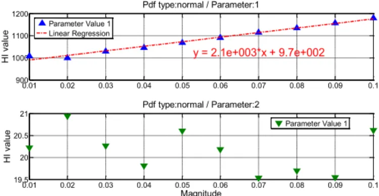
The following figure 8 shows how the damage model of Equ.25 is computed for parameter 1. This figure shows that parameter 1 is relevant to represent the system health status because it evolution with the degradation mode magnitude has a linear trend. However, parameter 2 does not shows any trend and consequently it is not representative of the system health status. As the system is composed of 6 degradation modes and 3 HI, 18 damage models are calculated.
Figure 8. Example of Damage Model Computation via linear regression of wHPSOV versus Magnitude for parameter 1
V. APPLICATION:RESULTS A. Degradation Modes Signatures
Thanks to the damage models, it is possible to compute the signatures of the degradation modes (c.f. Equ.8). The results for all the degradation modes are the following ones, with 𝑺𝒉𝑺𝒚 the simulated healthy syndrome:
𝑺𝒉𝑺𝒚 = |714903 61.720.9 1008 20.2 | (26) 500 600 700 800 900 1000 1100 1200 1300 500 600 700 800 900 1000 1100 1200 1300 Values of fi K ri g in g e stim a tio n o f f-i Cross-validation Scatterplot fi = estimated f-i curve
950 1000 1050 1100 1150 1200 1250 0 10 20 30 40 50 60 70 80 90 wHPSOV Magnitude = 0.01 Magnitude = 0.02 Magnitude = 0.03 Magnitude = 0.04 Magnitude = 0.05 Magnitude = 0.06 Magnitude = 0.07 Magnitude = 0.08 Magnitude = 0.09 Magnitude = 0.1 0.01 0.02 0.03 0.04 0.05 0.06 0.07 0.08 0.09 0.1 900 1000 1100 1200 Pdf type:normal / Parameter:1 Magnitude H I va lu e y = 2.1e+003*x + 9.7e+002 0.01 0.02 0.03 0.04 0.05 0.06 0.07 0.08 0.09 0.1 19.5 20 20.5 21 Pdf type:normal / Parameter:2 Magnitude H I va lu e Parameter Value 1 Linear Regression Parameter Value 1
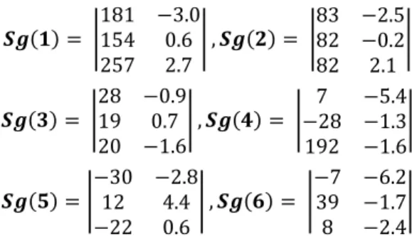
𝑺𝒈(𝟏) = |181 −3.0154 0.6 257 2.7| , 𝑺𝒈(𝟐) = | 83 −2.5 82 −0.2 82 2.1 | 𝑺𝒈(𝟑) = |28 −0.919 0.7 20 −1.6| , 𝑺𝒈(𝟒) = | 7 −5.4 −28 −1.3 192 −1.6| 𝑺𝒈(𝟓) = |−30 −2.812 4.4 −22 0.6| , 𝑺𝒈(𝟔) = | −7 −6.2 39 −1.7 8 −2.4| The bar plot of the first component of these syndromes (the mean) are presented in figure 9. The results given in this figure are obtained through simulations only but so it is necessary to replace them in a realistic framework. Thus, experts where asked to validate or invalidate these results by a physical approach. Their conclusions are the following:
Degradation modes 1 and 2 generate an increase of all the HI, which is physically explained by the fact that pump leakages create a loss of outlet fuel flow so a reduction of hydraulic power.
Degradation mode 4 generate a huge variation of HI 3 which can be explained by the fact that because of its internal leakage, the TBV utilizes more flow and so the remaining flow is not sufficient to move the HPSOV. The other variations are almost negligible and experts
have not seen any inconsistency.
Figure 9. Degradation mode signatures for the 3 HI. B. Recalibrated Healthy Syndrome
For this application, 195 datasets of HI measured on the real operational system are available. As they have been computed at the beginning of its operational life, it is supposed that they correspond to healthy behaviors. Figure 10 compares the measured and simulated healthy distribution of wBSV with their respective Gaussian fitting obtained by MLE. It can be noticed that despite their similarity, both the simulated mean and standard deviation are a little bit underestimated. The purpose of the syndrome recalibration is to fix this approximation.
Figure 10. Comparison between measured and simulated healthy distributions of HI wBSV with their gaussian fitting
The syndrome recalibration is done by using Equ.10 and knowing the MhSy and the maximal admissible degradation, it is possible to compute the RfSy:
𝑴𝒉𝑺𝒚 = |750945 79.915.2 1060 23.5| 𝑹𝒇𝑺𝒚(𝟏) = |1099 15.8931 76.9 1317 26.2 | , 𝑹𝒇𝑺𝒚(𝟐) = |1027 15.0833 77.4 1142 25.6 | 𝑹𝒇𝑺𝒚(𝟑) = |778964 15.979 1080 21.9| , 𝑹𝒇𝑺𝒚(𝟒) = | 757 74.5 917 13.9 1252 21.9 | 𝑹𝒇𝑺𝒚(𝟓) = |720957 77.119.6 1038 24.1| , 𝑹𝒇𝑺𝒚(𝟔) = | 743 73.7 984 13.5 1068 21.1| (27)
C. Detection and Identification Performance
In this section, it will be supposed that the specifications are the following ones:
{ 𝑇𝑃 > 80% 𝐹𝑃 < 5% ∀(𝑖, 𝑗) ∈ ‖1; 𝑑‖2, ∃𝑘 ∈ ‖1; 𝑟‖/ 𝐷 𝑘(𝑖, 𝑗) > 0.8 𝑟𝑎𝑑 (28) 1) Detection KPI
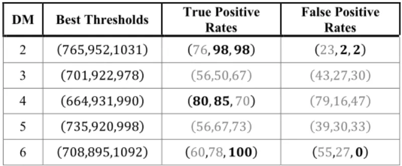
TP and FP are computed from MhSy and RfSy and their values are presented in table III for HI 1, 2 and 3. The results show that KPI of degradation modes 1, 2 and 6 are compliant with the specifications but HI are not sensitive enough to detect the others. However, as explained before, those degradation modes are not the critical ones because their occurrence rate is low. Eventually, the results traduce a good potential performances for detection.
TABLE III. DETECTION KPI–TP AND FPVALUES FOR BEST THRESHOLD
DM Best Thresholds True Positive Rates False Positive Rates
1 (810,986,1108) (𝟗𝟑, 𝟏𝟎𝟎, 𝟏𝟎𝟎) (𝟔, 𝟎, 𝟎) 1 2 3 4 5 6 -50 0 50 100 150 200 250 300 Degradation Mode H ea lth In dica to rs V alu es wBSV wTBV wHPSOV 5000 550 600 650 700 750 800 850 900 950 1000 10 20 30 40 50 60 wBSV Measured Distribution of wBSV Gaussian fitting obtained by MLE Simulated Distribution of wBSV Gaussian fitting obtained by MLE
DM Best Thresholds True Positive Rates False Positive Rates 2 (765,952,1031) (76, 𝟗𝟖, 𝟗𝟖) (23, 𝟐, 𝟐) 3 (701,922,978) (56,50,67) (43,27,30) 4 (664,931,990) (𝟖𝟎, 𝟖𝟓,70) (79,16,47) 5 (735,920,998) (56,67,73) (39,30,33) 6 (708,895,1092) (60,78, 𝟏𝟎𝟎) (55,27, 𝟎) 2) Identification KPI
Distinguishability vectors are computed for all the couples of degradation modes and the values in 𝑟𝑎𝑑 are presented in table IV. The results show that all the distinguishability vectors have at least one coefficient above the specification except for the couple (1; 2). However, as degradation modes 1 and 2 are located on the same equipment, it does not affect the localization. Moreover, the main validation criterion is that the critical degradation modes are identifiable from the others in order not to pollute their detection. Finally, as this criterion is verified in our case, results can be considered satisfactory.
TABLE IV. IDENTIFICATION KPI–DISTINGUISHABILITY VALUES
Degradation modes 1 2 3 4 5 6 1 |0 0| |0.220.21| |𝟏. 𝟕𝟐0.30| |𝟎. 𝟖𝟐𝟏. 𝟎𝟖| |𝟐. 𝟑𝟎𝟎. 𝟗𝟑| |𝟏. 𝟎𝟕𝟏. 𝟏𝟔| 2 |0.22 0.21| |00| |𝟏. 𝟕𝟔0.17| |𝟏. 𝟎𝟒𝟎. 𝟗𝟗| |𝟐. 𝟏𝟗𝟏. 𝟏𝟐| |𝟎. 𝟗𝟕𝟏. 𝟎𝟕| 3 |𝟏. 𝟕𝟐0.30| |𝟏. 𝟕𝟔0.17| |00| |𝟏. 𝟎𝟗𝟎. 𝟗𝟔| |𝟐. 𝟑𝟐𝟏. 𝟏𝟎| |𝟏. 𝟏𝟏𝟎. 𝟗𝟏| 4 |𝟎. 𝟖𝟐 𝟏. 𝟎𝟖| |𝟏. 𝟎𝟒𝟎. 𝟗𝟗| |𝟏. 𝟎𝟗𝟎. 𝟗𝟔| |00| |𝟐. 𝟐𝟓𝟏. 𝟐𝟗| |𝟏. 𝟓𝟐0.08| 5 |𝟐. 𝟑𝟎𝟎. 𝟗𝟑| |𝟐. 𝟏𝟗𝟏. 𝟏𝟐| |𝟐. 𝟑𝟐𝟏. 𝟏𝟎| |𝟐. 𝟐𝟓𝟏. 𝟐𝟗| |00| |𝟏. 𝟐𝟓𝟏. 𝟑𝟑| 6 |𝟏. 𝟎𝟕 𝟏. 𝟏𝟔| |𝟎. 𝟗𝟕𝟏. 𝟎𝟕| |𝟏. 𝟏𝟏𝟎. 𝟗𝟏| |𝟏. 𝟓𝟐0.08| |𝟏. 𝟐𝟓𝟏. 𝟑𝟑| |00| CONCLUSION
In this document, a hybrid approach for diagnostics based on the complementarity between model-based and data-driven technics has been introduced through some definitions and framework. Then, the principle of Kriging and its utility in time computational costs reduction was addressed. Eventually, the approach was tested on an aircraft engine pumping unit and had showed good results not only in computing the degradation modes signatures but also in evaluating detection and identification performances. However, this example was a simplified one and for future research, the main purpose is to extend the approach to the entire fuel system. The difficulty will then be to manage the large number of parameters and it will certainly be necessary to use some sensitivity analysis technics. In parallel, a further literature review on Kriging optimization and validation methods needs to be done in order to increase the quality of the models. Finally, Kriging was just
one surrogate modeling method among others and it would be interesting to perform a comparative study of all this technics.
REFERENCES [1] "OSA-CBM Website," [Online]. Available:
http://www.osacbm.org/.
[2] R. Isermann, «Model-Based fault-detection and diagnosis - status and applications,» Annual Reviews in Control, vol. 29, n° %11, pp. 71-85, 2005.
[3] H. Wang, T. Y. Chai, J. L. Ding et M. Brown, «Data Driven Fault Diagnosis and Fault Tolerant Control: Some Advances and Possible New Directions,» Acta Automatica Sinica, vol. 35, n° %16, p. 739–747, 2009.
[4] A. Garga, K. McClintic, R. Campbell, C. C. Yang, M. Lebold, T. Hay et C. Byington, «Hybrid Reasoning for Prognostic Learning in CBM Systems,» vol. 6, pp. 2957-2969, 2001. [5] S. Kumar, M. Torres, Y. C. Chan et M. Pecht, «A hybrid
prognostics methodology for electronic products,» chez Neural Networks, 2008. IJCNN 2008.(IEEE World Congress on Computational Intelligence). IEEE International Joint Conference on, 2008.
[6] E. De Rocquigny, N. Devictor, S. Tarantola, F. Mangeant, C. Schwob, R. Bolado-Lavin, J. R. Massé, P. Limbourg, W. Kanning and P. Van Gelder, Uncertainty in industrial practice: A guide to quantitative uncertainty management, Wiley, 2007. [7] T. D. Wickens, Elementary Signal Detection Theory, Oxford
University Press, 2002.
[8] A. I. J. Forrester et A. J. Keane, «Recent advances in surrogate-based optimization,» Progress in Aerospace Sciences, vol. 45, n° %11-3, pp. 50-79, 2009.
[9] F. A. Viana, G. Venter et V. Balabanov, «An algorithm for fast optimal Latin hypercube design of experiments,» International journal for numerical methods in engineering, vol. 82, n° %12, pp. 135-156, 2010.
[10] J. P. C. Kleijnen, «Kriging metamodeling in simulation: a review,» European Journal of Operational Research, vol. 192, n° %13, pp. 707-716, 2009.
[11] H. B. Nielsen, S. N. Lophaven et J. Sondergaard, DACE - A Matlab Kriging Toolbox, Lyngby - Denmark: Informatics and Mathematical Modelling, Technical University of Denmark, DTU, 2002.
[12] R. H. Myers, D. C. Montgomery et C. M. Anderson-Cook, Response surface methodology: process and product
optimization using designed experiments, Hoboken, New Jersey, USA,: Wiley, 2009.
[13] B. Lamoureux, J. R. Massé et N. Mechbal, «An Approach to the Health Monitoring of the Fuel System of a Turbofan,» chez IEEE Conference on Prognostics and Health Management (PHM), Denver (CO), 2012.
[14] P. Casoli, V. Andrea and G. Franzoni, "A Numerical Model for the Simulation of External Gear Pumps," in Proceedings of the 6th JFPS International Symposium on Fluid Power, Tsukuba, 2005.
[15] R. Frith and W. Scott, "Wear in external gear pumps : a simplified model," Wear 172, pp. 121-126, 1994.