Science Arts & Métiers (SAM)
is an open access repository that collects the work of Arts et Métiers Institute of
Technology researchers and makes it freely available over the web where possible.
This is an author-deposited version published in: https://sam.ensam.eu
Handle ID: .http://hdl.handle.net/10985/17947
To cite this version :
Alberto BADÍAS, Sarah CURTIT, David GONZÁLEZ, Iciar ALFARO, Francisco CHINESTA, Elías G. CUETO An augmented reality platform for interactive aerodynamic design and analysis -International Journal for Numerical Methods in Engineering - Vol. 120, n°1, p.125-138 - 2019
Any correspondence concerning this service should be sent to the repository Administrator : archiveouverte@ensam.eu
An augmented reality platform for interactive aerodynamic
design and analysis
Alberto Badías
1Sarah Curtit
1,2David González
1Icíar Alfaro
1Francisco Chinesta
3Elías Cueto
11Aragon Institute of Engineering
Research, Universidad de Zaragoza, Zaragoza, Spain
2Student, École Nationale des Ponts et
Chaussées, Champs-sur-Marne, France
3ESI Group Chair at Procédés et
Ingénierie en Mécanique et Matériaux (PIMM), ENSAM ParisTech, Paris, France
Correspondence
Elías Cueto, Aragon Institute of Engineering Research, Universidad de Zaragoza, Edificio Betancourt, Maria de Luna, s.n., 50018 Zaragoza, Spain. Email: ecueto@unizar.es
Funding information
ESI Group; Spanish Ministry of Economy and Competitiveness, Grant/Award Number: DPI2015-72365-EXP; Regional Government of Aragon; European Social Fund
Summary
While modern CFD tools are able to provide the user with reliable and accu-rate simulations, there is a strong need for interactive design and analysis tools. State-of-the-art CFD software employs massive resources in terms of CPU time, user interaction, and also GPU time for rendering and analysis. In this work, we develop an innovative tool able to provide a seamless bridge between artistic design and engineering analysis. This platform has three main ingredients: com-puter vision to avoid long user interaction at the pre-processing stage, machine learning to avoid costly CFD simulations, and augmented reality for an agile and interactive post-processing of the results.
K E Y WO R D S
augmented reality, CFD, interactivity, machine learning, real time
1
I N T RO D U CT I O N
Very much like other aspects of our everyday life, simulation is living profound changes. It is not infrequent to hear about “democratization”—more than deployment—of simulation or even about appification. In general, by democratization, we mean to make simulation accessible to users that previously did not feel the need for it, but now consider it interesting. However, many undoubtedly interesting applications of simulation in engineering practice come at the price of many hours of user interaction followed by many CPU hours to obtain results, and this results in a barrier for many potential users.
In industry, particularly in automotive manufacturing, there is a claim for interactive ways to connect designers (artists, in sum) and engineers.1For this to be possible, developing real-time, interactive simulation apps that could provide imme-diate responses on the physical effects of purely artistic decisions on mockups, for instance, could be of great help. This immediacy and interactivity should include the pre-processing stage in which engineers construct the CAE model of the product and the meshing operation for the development of a FEA model and a reasonable time to response.
In parallel, with the global deployment of mobile devices (smartphones, tablets), there is a tendency toward simulation
appification, ie, the implementation on such platforms of the usual simulation tools. While the performance of these platforms is nowadays impressive, they are undoubtedly less powerful than usual workstations. This imposes additional requirements to any realistic attempt to simulation democratization.
Augmented reality (AR) has gained popularity given the realism and ease of interpretation of the information it pro-vides. Therefore, AR can now be seen as a feasible way for simulation post-processing. However, AR makes intensive use of computer vision techniques2,3and therefore induces additional restrictions to the simulation pipeline.4
In this work, we present our first attempt to democratize simulation by developing a platform that copes with the afore-mentioned requirements. We try to directly suppress the user time employed in the construction of the model. Instead, it is required that the model comes directly from physical reality, through computer vision techniques. As a proof of con-cept, we focus on car aerodynamics, and thus, the geometry of the car (or prototype) will be captured by a commodity camera. No stereo or RGBD cameras are needed, in principle, even if their use is obviously possible and could eventually ease and improve the accuracy of the process. Previous approaches to this problem employ this type of cameras (Microsoft Kinect cameras, for instance, in the work of Harwood et al,5that capture depth measures by means of an infrared laser). Geometry of the objects to analyze will thus be acquired by computer vision, thus bypassing the need for time-consuming CAE pre-processing steps. Usually, the same device that captures geometry will serve to depict the results in an AR framework, but many different possibilities exist. Our approach makes use of feature-based Simultaneous Local-ization and Mapping (SLAM) techniques to acquire the geometry of the object with a single monocular camera, even though many modern smartphones are already equipped with stereoscopic cameras. In particular, we employ ORB-SLAM techniques.6These techniques allow us to capture selected points on the surface of the object, whose geometry will need, nevertheless, to be reconstructed from these points. In other words, a suitable parameterization of the shape of the object needs to be constructed. Previous works include the use of free-form deformation techniques7 or the closely related approach in the work of Umetani and Bickel.8
Our approach to the problem is data-driven.9-14This means that we employ manifold learning techniques15over a data base of previously computed CFD results. While there is a vast corps of literature on (linear) model reduction of flow problems,16-22 these techniques rarely achieve real-time performance. For this particular application, by real-time we mean a code able to provide feedback response at some 30 to 60 Hz (ie, the usual number of frames per second in modern smartphone cameras).
Other approaches, however, achieve interactivity by means of machine learning8or by model reduction1 but do not consider AR output. On the other side of the spectrum, some previous studies have considered the brute force approach.5 This type of approach makes intensive use of GPUs capabilities in a Lattice Boltzmann framework and are not well suited, therefore, for their implementation on a mobile platform.
The employ of machine learning toward learning physical dynamics has gained considerable interest in recent times.23-25In particular, deep learning architectures are of course tempting.26 In general, while model order reduction methods27,28achieve important speedup by means of a considerable reduction in the number of degrees of freedom and also provide with important insight on the physics of the problem, deep learning architectures perform in nearly the oppo-site way.29They are able to capture multiscale phenomena or transient features and, at the same time, are able to capture invariants of the system, but need for a tremendous effort to train the neural networks and, conversely, provide little or no interpretation of the results. Some scientists have warned about the possible implications that the employ of machine learning on top of biased data could have.30
Closely related, there is a strong research activity in the development of physics-aware artificial intelligence—in other words, machine learning approaches that satisfy first principles by construction.31-33Our approach here is to employ, so to speak, the best of both worlds. Nonlinear dimensionality reduction techniques—in particular, manifold learning—are able to substantially reduce the number of degrees of freedom of the problem, very much like classical, linear model order reduction. However, at the same time, these provide very useful insight on the nonlinearity of the problem. As will be noticed from the results here presented, manifold learning techniques provide clear physical explanations on the structure of data, reduce the number of degrees of freedom and their dimensionality, and allow for very efficient computational approaches.
With all these ingredients—computer vision, machine (manifold) learning and AR—we construct a reliable simulation platform that, even if we admit errors higher than those typical of state-of-the-art high-fidelity simulations, provide the user with a unique degree of interactivity and immediacy.
This paper is structured as follows. In Section 2, we provide an overall description of the method we have devel-oped. In Section 3, we give detailed insight on the construction of the database and its subsequent embedding in a lower-dimensional space. Then, in Section 4, we briefly describe the state-of-the-art computer vision techniques employed to capture cars not being in the database. In Section 5, we describe how to interactively depict CFD results on top of the video stream of the particular car of interest. Finally, in Section 6, we analyze the accuracy of the results, computational cost, etc. This paper is completed with some final comments about the interest of the proposed technique.
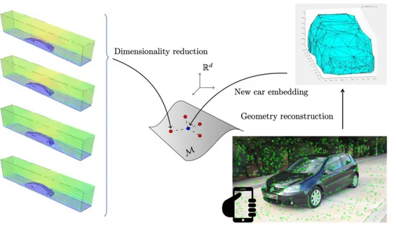
FIGURE 1 Schematic description of the method. We first construct a database of CFD results for known car
geometries (left column). These results are embedded onto a low-dimensional manifold by means of locally linear embedding techniques. Once a new car—not in the
database—is captured with the camera, the features are first processed so as to obtain an approximate envelope of the new car geometry. This new geometry is then embedded onto the manifold (blue point) and its CFD results interpolated among its neighbors in the manifold (red points)
2
OV E R A L L D E S C R I P T I O N O F T H E M ET H O D
Figure 1 depicts a sketch of the general pipeline of the method. The key ingredient is the employ of manifold learning techniques to learn car aerodynamics. This will allow us to avoid simulating in real time. Instead, we interpolate—in the right manifold space—existing CFD results (represented in the left column of Figure 1). By obtaining a low-dimensional embedding of these results, we will not only ensure to interpolate in the right space (instead of the Euclidean one) but also take profit of the nonlinear reduced order modeling capabilities of locally linear embedding (LLE) techniques,34which will be thoroughly described in Section 3.
These results are obtained by usual CFD methodologies, starting from CAD descriptions of car bodies. Once unveiled, the manifold structure of these data,, will allow us to easily incorporate new designs, not previously analyzed (right column of Figure 1). With the help of a standard smartphone, we will capture the bodywork of a new car or prototype. To this end, it is necessary to film around the car, so as to capture its entire geometry. SLAM techniques6will allow us to detect special points in the body of the car called ORB features (green points in the bottom-right corner of Figure 1).35
After a reconstruction of the body of the car from these ORB points (top right corner of Figure 1), we are in the position of embedding this new design onto the already available manifold of shapes. This will also provide us with the necessary weights so as to interpolate from surrounding CFD results in the database. This simple approach will allow us to obtain velocity maps, streamlines, etc. without the burden of meshing procedures, long CPU computations and subsequent post-processing.
Once the new results have been obtained, they are ready to be represented on the screen, on top of the video stream. For this to be possible, a registration process will be needed. By image registration, we mean the process of finding the common system of reference between the video frames and the just obtained CFD results. So to speak, we need to align both so as to construct an AR post-processing of these results.
These steps are detailed in the following sections. We begin by describing the steps toward the obtention of the car database.
3
CO N ST RU CT I O N O F A S U I TA B L E DATA BA S E O F C F D R E S U LT S
3.1
Parameterization of the shape
A crucial step in the machine learning of car aerodynamics is that of parameterizing shape. This issue has been deeply analyzed in the work of Umetani and Bickel,8for instance. In the reduced order modeling literature, there is another
FIGURE 2 Model de-refinement for the Ford Fiesta example
vast corps of literature7,17,20,36,37for works employing freeform deformation techniques. Of course, usual CAD techniques based on the employ of NURBS or related approaches cannot be employed here, since the capture of shapes by computer vision is obliged in the tool we are developing. This problem shares many similarities, for instance, with the construction of patient avatars in the medical community.38-40
The original database was composed by object (*.obj) files. Prior to converting them to a manageable format, com-patible with the computer vision system, a de-refinement of the bodywork of every analyzed model is mandatory, see Figure 2. We employed the same de-refinement method as in the work of Umetani and Bickel.8In the examples analyzed herein, the intermediate level of refinement was chosen that corresponds with the center figure in Figure 2. Of course, the final accuracy of the method strongly depends on the level of detail to which the body of the car is represented. Further refinement leads of course to higher levels of accuracy.
This de-refined geometry is then embedded into a grid of 140 × 40 × 20 points uniformly distributed on a volume of 14 × 5 × 4 cubic meters around each half car (we exploit here the symmetry of cars so as to include only one half of the bodywork in the database). While in some of the previous works of the authors,38we employed a signed distance field to characterize the shape, in this work, we have found that the employ of a presence function
𝜙(x) =
{
1 if x ∈ Ω,
0 if x ∉ Ω, (1)
where Ω represents the boundary of the car, rendered better results for the manifold learning procedure to be described next. In other words, we characterized each particular shape by a vector z ∈ ℝD, where D = 140 × 40 × 20 = 112 000,
whose entries are the values of𝜙(xj)at each node of the grid, xj, j = 1, … , 112 000.
3.2
Manifold learning
The key ingredient in our method is to hypothesize that car shapes describe a manifold structure whose precise form is to be found. To this end, we employ LLE techniques.34In essence, LLE assumes that, given the fact that a manifold is homeomorphic to a flat space in a sufficiently small neighborhood of each point, each datum can be reasonably well approximated through a linear combination of its nearest neighbors—whose precise number M is to be fixed by the user. Therefore, LLE assumes that, for each zm, a linear reconstruction exists of the form
zm=
∑
i∈m
Wmizi, (2)
where Wmiare the unknown weights andmthe set of the M-nearest neighbors of zm.
The search for the weights is done by minimizing the functional
(W) = M ∑ m=1 ‖‖ ‖‖ ‖‖zm− M ∑ i=1 Wmizi ‖‖ ‖‖ ‖‖ 2 ,
where Wmiis zero if zi∉m, ie, if cars i and m are not neighbors in the manifold of shapes.
LLE also hypothesizes that an embedding exists onto a lower-dimensional spaceℝd, with d≪ D, such that the manifold
FIGURE 3 Hypothesis abut the existence of a manifold on which the car shapes live. The small black dots represent the car database in a high-dimensional spaceℝD. These data are then embedded onto a lower-dimensional manifoldℝd, with d≪ D. A new car not in the database (blue dot) will thus be interpolated from its neighboring cars (red points) through the weights Wmiprovided by locally linear embedding (LLE) that define a mapping
ℤ(𝝃). By hypothesis, LLE assumes that the same neighborhood relationships hold in the high-dimensional manifold
by minimizing a new functional
(𝝃1, … , 𝝃M) = M ∑ m=1 ‖‖ ‖‖ ‖‖𝝃m− M ∑ i=1 Wmi𝝃i ‖‖ ‖‖ ‖‖ 2 ,
where the neighboring relation between points (ie, the weights Wmi) are maintained. See Figure 3 for a description of LLE.
3.3
Our database
We analyzed a set of 80 different car bodies. All of them are subjected to a CFD analysis using commercial software. Figure 4 shows a typical mesh of the environment of one of the models. All of them are subjected to a uniform velocity of 10 m/s at the leftmost part of the meshed volume. This gives us a Reynolds number on the order of 9000.
After the CFD computations, a projection of the velocity field onto the same grid mentioned in Section 3.1 is made for subsequent interpolation purposes. Our cars are then manually classified into four different groups: large cars (Audi Q7, Hummer, Jeep Grand Cherokee, VW Touareg, among others), sports cars (Mercedes AMG GTS, BMW Z4, Audi R8, BMW i8, Porsche 911, … ), old cars (Pontiac firebird, Dodge Charger, Chevrolet Camaro, … ), and a fourth set of “various,” which comprises not easily classifiable models.
FIGURE 4 (A) Typical FE mesh employed in the CFD calculations. (B) Contour plot of the velocity module for the same model
FIGURE 5 Results of the embedding of car geometries ontoℝ2by
employing nine neighbors for each car. It can be noticed how locally linear embedding clusterizes sports cars far apart familiar (or “large”) cars, while old cars and other models without a distinctive characteristic are somehow mixed
Our experiments showed that a range between M = 6 − 15 neighbors provided a good embedding ontoℝ2. Figure 5 shows the embedding obtained with M = 9 neighbors, where it can be noticed how LLE clearly clusterizes sports cars apart from large, familiar cars, for instance. Old cars, whose shape does not follow any specific pattern, and those cars in the “various” group are somewhat mixed in the embedding procedure, as expected.
4
CO M P U T E R V I S I O N FO R N E W C A R M O D E L S
While the previous sections described the offline work to construct the car database, in the following section, we describe the online work done for the characterization of the new geometry and the subsequent interpolation of the results on the manifold of shapes.
After the database has been completed, and its dimensionality conveniently reduced, the pipeline of our platform faces the problem of reconstructing the geometry of a new car. In general, a new car or a new design will not be in the database, so we assume that no CAD description is available. Instead, the user will make use of a commodity camera (through a smartphone, for instance) to capture the new geometry.
4.1
Capturing the geometry from a video sequence
The problem of reconstructing a three-dimensional (3D) geometry from a set of two-dimensional (2D) images is known in the robotics field as the Structure from Motion, SfM, problem.2,41,42In essence, if we assume that the object to reconstruct is rigid—for the deformable case, refer to our other work4and references therein—the problem is sketched in Figure 6. The object is assumed to be attached to a fixed position in the frame of reference. The problem thus begins by determining the pose—location and orientation—of the camera.
The input image space is denoted byk⊂ℝ2, with k = 1, … , nimages, the number of available frames in the just captured video. We assume no batch approach in this platform but we do not consider the possibility of a video stream. In other words, the video has a finite number of frames.
Cameras perform a projection from 3D, physical space to a 2D pixel space. This projection is characterized by an a priori unknown camera operator denoted by Π ∶ 𝜕∗Ω
t → whose determination is known as the calibration of the camera.
This projection can be expressed as Π = K[R|t], where K corresponds to the camera intrinsic matrix and [R|t] represents the camera extrinsic matrix. We denote x = (x, y, z)⊤and p = (p1, p2)⊤and a scale factor s, so that,
[ p1 p2 s ] =𝜆 ⎡ ⎢ ⎢ ⎣ 𝑓∕d x 0 cx 0 𝑓∕d𝑦 c𝑦 0 0 1 ⎤ ⎥ ⎥ ⎦ [ R t ] ⎡ ⎢ ⎢ ⎢ ⎣ x 𝑦 z 1 ⎤ ⎥ ⎥ ⎥ ⎦ ⏟⏞⏞⏞⏞⏟⏞⏞⏞⏞⏟ xc , (3)
where xcrepresents the coordinates of x in the camera system (a moving frame of reference attached to the camera, not
FIGURE 6 Sketch of the structure from motion problem. While the object is assumed to be rigid and attached to a fixed position in the frame of reference, the camera needs to move so as to reconstruct its three-dimensional geometry. Here, two video frames, namely,1
andn, are shown, together with the camera projections of the solid. The projection Π of a particular point x on the visible surface of the solid gives rise to point p in the pixel space [Colour figure can be viewed at wileyonlinelibrary.com]
Two transformations exist: first, the camera extrinsic matrix transforms 3D physical points in the world system of ref-erence into 3D points in the camera moving frame of refref-erence. This transformation is equivalent to the composition of a rotation (R) and translation (t) between the corresponding points. On the other hand, the camera intrinsic matrix K con-tains information about the projection center (cx, cy), the pixel size (dx, dy), and the focal distance, f, that maps 3D camera
points into 2D pixel coordinates. Finally,𝜆 represents a scale factor that takes into account the fact that, with a single picture, an indeterminacy exists that makes it impossible to discern between the projection of a big object positioned far from the objective or a small one at a closer position.
Therefore, to determine the camera pose and the location of a rigid object, we need more than one single image. To solve this indeterminacy, SfM algorithms minimize the reprojection error. In other words, SfM minimizes the geometric error corresponding to the image distance between a projected point and a measured one.3As sketched in Figure 6, the camera performs a projection of the form
p = Π(x),
with p ∈ ℝ2 and x ∈ ℝ3. Note that we do not know the exact value of x. Well-established geometrical analysis will provide an estimation̂x of the true position of the point.3,43If we reproject this estimate for each frame by
̂p = Π(̂x),
the sought reprojection error takes the form d( p, ̂p).
This analysis is often made with respect to some marked points usually known as fiducial markers. In general, this analysis is greatly simplified if the object to reconstruct can be labeled at some points with the help of some visible sticker, for instance. However, for our purpose, this is not feasible. The tracked points x must be selected by the algorithm itself. To this end, we employ a method based on features, the so-called Oriented FAST and rotated BRIEF (ORB) method.35In fact, we employ the so-called ORB-based SLAM (ORB-SLAM) method, able to solve the SfM problem while, at the same time, it constructs a map of the environment.6These ORB features are the green points shown in Figure 7.
4.2
Projection onto the database
The ORB features just captured constitute a cloud of points in the boundary of the sought geometry. To determine the best possible approximation to the sought geometry, we employ𝛼-shapes.44Essentially,𝛼-shapes reconstruct a volume given a cloud of points on its boundary with the help of one user-defined parameter,𝛼, that represents the coarsest level of detail in the reconstructed geometry. Basically,𝛼 is on the order of the distance between recognized ORB features.
Of course, a stereo or RGBD camera would provide a much more detailed geometry representation. We analyze, how-ever, the case of deployed hardware and consider that a simple smartphone or tablet is enough to obtain a reasonable representation of each car bodywork. With the just reconstructed geometry, we embed it in the same grid employed to construct the car database and evaluate the presence function𝜙(x) at each of the nodes of the grid, xj, j = 1, … , D, see
FIGURE 7 (A) An example of the captured ORB features for the VW Golf model. (B) A reconstruction of the camera movements in the video. Blue pyramids indicate the position and orientation (pose) of the camera. Dots represent the ORB's detected by the SLAM methodology that belong both to the car and its surroundings. ORB, Oriented FAST and rotated BRIEF; SLAM, Simultaneous Localization and Mapping
FIGURE 8 The car's geometry is then embedded on a grid and the presence function, Equation (1), evaluated at each of its nodes. Red nodes are evaluated to zero (they fall outside of the car) while blue ones are evaluated to one (they fall inside). Note that the grid's resolution is lower than that actually employed (140 × 40 × 20) just to make the figure visible
This new vector znewcan easily be embedded on the manifold without the need of recomputing every weight, by invok-ing incremental LLE algorithms, see the work of Schuon et al,45 for instance. This will provide the new weights W
i,
i =1, … , M.
The key ingredient in our method is the assumption that the velocity field (for sufficiently low Re numbers) of a new car can be obtained in an accurate enough manner by linear interpolation among the neighboring models in the manifold.
In other words, the new velocity field is approximated by vnew(x 𝑗) ≈ M ∑ i=1 Wivi(x𝑗), (4)
with vi(xj)being the velocity field for the ith neighboring car model at the jth node of the grid. This assumption, which may
seem too restrictive, has demonstrated already to provide reasonably accurate results in a completely different context, but in a similar procedure, see our previous work.38
5
AU G M E N T E D R E A L I T Y O U T P U T
5.1
Car identification
ORB-SLAM is probably the best technique to reconstruct static 3D scenes in a sparse way, if we think of employing a commodity camera. We can estimate the 3D position x(x, y, z) of the most relevant points of a scene, extracted by using the feature descriptor ORB. This means that we need a relatively low computational power to work; it does not require the use of graphical acceleration by GPU, at the cost of reducing the number of observed points. With this system, we do not expect to obtain a dense cloud of points, as it happens with other acquisition systems (such as RGB-D devices or stereo systems), but to be able to take very precise measurements in real time with little computational cost. It is also important to point out that densification techniques can be applied a posteriori to obtain a denser 3D point cloud, such as the work of Mahmoud et al.46
Since we are using a monocular system (like the camera we can have in our smartphone), we cannot recover the scale of the model without knowing any of the real dimensions of the objects (an RGB-D system or stereo camera could give us this information, but a standard user does not usually have this type of technology). Nor can we identify the direction of gravity (it could be done with an Inertial Measurement Unit or IMU), which complicates the estimation of the location or pose of the car in space. Our objective is to depend only on the visual system, obtaining the information of the scene from only a monocular camera.
We start, therefore, from a set of 3D points estimated in the scene, where we need to identify the geometry of a car. For this, we assume that the user has surrounded a real car with its monocular system, where the car appears relatively centered in the cloud of points. Figure 9 collects the algorithm used to identify, segment, and locate the position of the car from the point cloud.
The first task of the algorithm is a point culling process depending on the local density surrounding any point of the cloud. We use this type of cleaning methods because sparse SLAM methods can add noise in the triangulation step. The use of a pyramid of image scales may also encourage this type of defects.
Next, we estimate the centroid of the cleared point cloud, which allows us to locate where the most relevant object in the scene is located. After this, we eliminate those points that are further away from 95% of the distances of all points from the centroid. This allows us to work without the need to add adjustment parameters.
We then estimate the plane of the ground, because we assume that the car is located on a large plane with texture. Thus, we estimate the main floor plane and remove the points contained in that plane.
A principal direction analysis is then applied to estimate the predominant direction of the vehicle that, with the centroid and the gravity vector (estimated from the floor plane), allows us to fix the coordinates origin of the car.
FIGURE 10 Final appearance of the augmented video. (A) Streamtraces can be plotted on top of the reconstructed geometry. (B) Other possibilities, such as pressure or velocity contour plots, also exist
The last step is the scaling. A noise removing process is again applied based in the histogram of positions to remove areas of isolated points. Then, the car is inserted within a box to facilitate the estimation of scale and geometric transformations, which are then applied to move the car to the origin of coordinates and scale it with a unitary scale. We can do this because although we do not recover the scale, if the camera is well calibrated, the system is able to obtain a very precise
3D aspect ratiobetween the 3 dimensions. In other words, even if the object is in another scale, moved and oriented in another direction, it is not necessary to apply different scales in the X-, Y-, or Z-axes, but a common scale of type
xSC(x, y, z) = 𝜆(xORB(x, y, z)), where xSCare the 3D positions of the geometry with scale correction and xORB(x, y, z) are the initial 3D coordinates estimated by the SLAM system. This allows us to compare the estimated car with the database of the rest of the cars, where we have already precomputed the aerodynamic solution.
It is important to note that we could also have used modern techniques of recognition of car pose through images only, employing learning techniques.47,48However, we think that it is possible that they do not reach the level of precision we expect for the geometry of a car. In addition, with our method, we avoid the labeling and training phase. Working with image masks and then estimating the position of the 3D points by triangulation may involve similar noise problems, and some points could be located outside the real geometry of the car. Therefore, we should apply some filtering techniques again, as we have done in our proposed method. The tests we have done show that, although we use classic techniques in our method, they work in a robust way.
5.2
Final appearance
The previous identification algorithm provides very valuable information for the final augmentation of the video. In par-ticular, having the reconstructed 3D geometry is a necessary step for the computation of occlusion culling in the results, ie, disabling objects not seen by the camera to appear in the image. All the steps in the augmentation process are implemented in OpenGL.49The final appearance of the augmented results is shown in Figure 10.
6
A NA LY S I S O F T H E R E S U LT S
In this section, we analyze the performance of the just presented methodology. Particular emphasis is made to the com-putational cost and real-time compliance of the online computations. A supplemental video showing both the process and the result of the proposed methodology can be downloaded from https://youtu.be/Azm4E3Y7jS4.
−0 .2 0 0.2 −0 .4 −0 .2 0 0.2 0.4 0.6 −0 .2 0
FIGURE 11 Reconstruction of the VW Golf model. Red points represent to detected ORB features. The blue volume is reconstructed by an𝛼-shape algorithm. ORB, Oriented FAST and rotated BRIEF
6.1
Computer vision
The first part of the online procedure is the capture of the bodywork geometry through ORB-SLAM techniques. This algorithm runs in real time (ie, it attains 30 to 60 frames per second) without any problem on a standard laptop. We employ the standard implementation in the work of Mur-Artal and Tardós,50whose code is freely available.
6.2
Reconstruction of the geometry
Given the set of points captured in the process described in the previous section, the reconstruction of the geometry of the bodywork (ie, the determination of the approximate geometry shown in Figure 11) takes on average 0.30 seconds in a MacBook Pro 2016 computer equipped with 16 Gb RAM running an Intel Core i7 processor at 3.3 GHz.
6.3
Embedding of the new model
After the reconstruction of the geometry, the new model or prototype should be embedded onto the manifold of shapes. This allows us to obtain the interpolation weights Wi, see Equation (4). This process takes, on average, less than a second.
Previous works have also reported how fast the LLE algorithm is, with some 500 different geometries running in about one second.38
6.4
Car identification
The procedure sketched in Figure 9 runs in real time on a standard laptop.
6.5
Error analysis
To test the accuracy of the LLE embedding onto the shape manifold, we deliberately kept five models out of the database. They were employed as ground truth, and their direct numerical simulation was compared to the result obtained by the interpolation of their velocity field, see Equation (4). L2-norm errors ranged from 1.02% for the Hummer model to 0.56% for a classic car labeled as sedan 4, see Figure 12.
These results indicate that, for the scale of the grid employed in the characterization of geometry, many models provide very similar results. These velocity fields are, therefore, easy to interpolate. A highly refined mesh—which is not necessary
FIGURE 12 Interpolated velocity field for the sedan 4 model. View along the symmetry plane [Colour figure can be viewed at wileyonlinelibrary.com]
for the type of applications we are envisaging here—would maybe report more important differences in the velocity field among different models.
7
CO N C LU S I O N S
We have presented a tool able to capture and reconstruct, with the help of a commodity camera, the geometry of a 3D object—we have studied mainly cars—and to perform simple but reasonably accurate CFD predictions of the flow around the object for interactive design. This technique employs state-of-the-art structure from motion techniques for the geomet-rical reconstruction and manifold learning techniques to construct inexpensive predictions of the velocity and pressure fields around the object.
The advantage of such a platform is that what we obtain is actually an appification of CFD software. This tendency in our community is having tremendous commercial implications and is changing the way we see simulation. Here, the user needs only a smartphone to capture the geometry of the object to analyze, so as to obtain timely information about the physical consequences of his or her decisions. Artistic designers are thus invited to incorporate CFD to their workflow in a seamless way and with a minimum of knowledge in engineering—something that could be risky, nevertheless.
The combination of computer vision techniques, artificial intelligence (here, manifold learning), and AR gives rise to a platform that changes the way we interact with simulation software. At the price of a little loss in accuracy with respect to existing high-fidelity software, we obtain real-time responses to our query in a very short period of time, thus enabling decision making and an easy interplay between designers and engineers.
AC K N OW L E D G E M E N T S
This project has been partially funded by the ESI Group through the ESI Chair at ENSAM ParisTech and through the project “Simulated Reality” at the University of Zaragoza. The support from the Spanish Ministry of Economy and Com-petitiveness through grant number DPI2015-72365-EXP and from the Regional Government of Aragon and the European Social Fund are also gratefully acknowledged.
O RC I D
Elías Cueto https://orcid.org/0000-0003-1017-4381
R E F E R E N C E S
1. Bertram A, Othmer C, Zimmermann R. Towards real-time vehicle aerodynamic design via multi-fidelity data-driven reduced order mod-eling. Paper presented at: 2018 AIAA/ASCE/AHS/ASC Structures, Structural Dynamics, and Materials Conference; 2018; Kissimmee, FL.
2. Szeliski R. Computer Vision: Algorithms and Applications. London, UK: Springer International Publishing; 2010. 3. Richard H, Andrew Z. Multiple View Geometry in Computer Vision. Cambridge, UK: Cambridge University Press; 2003.
4. Badías A, Alfaro I, González D, Chinesta F, Cueto E. Reduced order modeling for physically-based augmented reality. Comput Methods
Appl Mech Eng. 2018;341:53-70.
5. Harwood ARG, Wenisch P, Revell AJ. A real-time modelling and simulation platform for virtual engineering design and analysis. In: Proceedings of 6th European Conference on Computational Mechanics (ECCM 6) and 7th European Conference on Computational Fluid Dynamics (ECFD 7); 2018; Glasgow, UK.
6. Mur-Artal R, Montiel JMM, Tardós JD. ORB-SLAM: a versatile and accurate monocular SLAM system. IEEE Trans Robot. 2015;31(5):1552-3098.
7. Lassila T, Rozza G. Parametric free-form shape design with PDE models and reduced basis method. Comput Methods Appl Mech Eng. 2010;199(23):1583-1592.
8. Umetani N, Bickel B. Learning three-dimensional flow for interactive aerodynamic design. ACM Trans Graph. 2018;37(4):89:1-89:10. 9. Ghnatios C, Masson F, Huerta A, Leygue A, Cueto E, Chinesta F. Proper generalized decomposition based dynamic data-driven control
of thermal processes. Comput Methods Appl Mech Eng. 2012;213-216(0):29-41.
10. Kirchdoerfer T, Ortiz M. Data-driven computational mechanics. Comput Methods Appl Mech Eng. 2016;304:81-101.
11. Ibañez R, Borzacchiello D, Aguado Jose V, et al. Data-driven non-linear elasticity: constitutive manifold construction and problem discretization. Computational Mechanics. 2017;60(5):813-826.
12. Lam RR, Horesh L, Avron H, Willcox KE. Should You Derive, Or Let the Data Drive? An Optimization Framework for Hybrid First-Principles Data-Driven Modeling. arXiv preprint arXiv:1711.04374. 2017.
14. Latorre M, Montáns Francisco J. What-you-prescribe-is-what-you-get orthotropic hyperelasticity. Computational Mechanics. 2014;53(6):1279-1298.
15. Lee JA, Verleysen M. Nonlinear Dimensionality Reduction. New York, NY: Springer Verlag; 2007.
16. Díez P, Zlotnik S, Huerta A. Generalized parametric solutions in Stokes flow. Comput Methods Appl Mech Eng. 2017;326:223-240. 17. Manzoni A, Quarteroni A, Rozza G. Model reduction techniques for fast blood flow simulation in parametrized geometries. Int J Numer
Methods Biomed Eng. 2012;28(6-7):604-625.
18. Rozza G, Huynh DBP, Patera AT. Reduced basis approximation and a posteriori error estimation for affinely parametrized elliptic coercive partial differential equations: application to transport and continuum mechanics. Arch Comput Methods Eng. 2008;15(3):229-275. 19. Manzoni A, Quarteroni A, Rozza G. Computational reduction for parametrized PDEs: strategies and applications. Milan J Math.
2012;80:283-309.
20. Manzoni A, Quarteroni A, Rozza G. Shape optimization for viscous flows by reduced basis methods and free-form deformation. Int J
Numer Meth Fluids. 2012;70(5):646-670.
21. Amsallem D, Cortial J, Farhat C. Towards real-time CFD-based aeroelastic computations using a database of reduced-order information.
AIAA Journal. 2010;48:2029-2037.
22. Amsallem D, Farhat C. An interpolation method for adapting reduced-order models and application to aeroelasticity. AIAA Journal. 2008;46:1803-1813.
23. Chang Michael B, Ullman T, Torralba A, Tenenbaum Joshua B. A compositional object-based approach to learning physical dynamics. CoRR. 2016. https://doi.org/abs/1612.00341
24. Bright I, Lin G, Kutz JN. Compressive sensing based machine learning strategy for characterizing the flow around a cylinder with limited pressure measurements. Phys Fluids. 2013;25(12):127102.
25. Ladický L, Jeong S, Solenthaler B, Pollefeys M, Gross M. Data-driven fluid simulations using regression forests. ACM Trans Graph. 2015;34(6). Article No. 199.
26. Oliehoek FA. Interactive learning and decision making: foundations, insights and challenges. In: Proceedings of the 27th International Joint Conference on Artificial Intelligence; 2018; Stockholm, Sweden.
27. Chinesta F, Cueto E. PGD-Based Modeling of Materials, Structures and Processes. Cham, Switzerland: Springer International Publishing; 2014.
28. González D, Masson F, Poulhaon F, Cueto E, Chinesta F. Proper generalized decomposition based dynamic data driven inverse identification. Math Comput Simul. 2012;82:1677-1695.
29. Kutz JN. Deep learning in fluid dynamics. J Fluid Mech. 2017;814:1-4.
30. Ghosh P. AAAS: Machine learning 'causing science crisis'. BBC News. February 16, 2019. https://www.bbc.com/news/science-environment-47267081. Accessed 2019.
31. Swischuk R, Mainini L, Peherstorfer B, Willcox K. Projection-based model reduction: Formulations for physics-based machine learning.
Comput Fluids. 2019;179:704-717.
32. Raissi M, Perdikaris P, Karniadakis GE. Physics Informed Deep Learning (Part I): Data-driven Solutions of Nonlinear Partial Differential Equations. arXiv preprint arXiv:1711.10561; 2017.
33. González D, Chinesta F, Cueto E. Thermodynamically consistent data-driven computational mechanics. Continuum Mech Thermodyn. 2019;31(1):239-253. https://doi.org/10.1007/s00161-018-0677-z
34. Roweis ST, Saul LK. Nonlinear dimensionality reduction by locally linear embedding. Science. 2000;290(5500):2323-2326.
35. Rublee E, Rabaud V, Konolige K, Bradski G. ORB: an efficient alternative to SIFT or SURF. Paper presented at: 2011 International Conference on Computer Vision; 2011; Barcelona, Spain.
36. Ballarin F, Manzoni A, Rozza G, Salsa S. Shape optimization by free-form deformation: existence results and numerical solution for Stokes flows. J Sci Comput. 2014;60(3):537-563.
37. Quarteroni A, Rozza G. Optimal control and shape optimization of aorto-coronaric bypass anastomoses. Math Models Methods Appl Sci. 2003;13(12):1801-1823.
38. González D, Cueto E, Chinesta F. Computational patient avatars for surgery planning. Ann Biomed Eng. 2015;44(1):35-45.
39. Lassila T, Manzoni A, Quarteroni A, Rozza G. A reduced computational and geometrical framework for inverse problems in hemodynam-ics. Int J Numer Methods Biomed Eng. 2013;29(7):741-776.
40. Zimmer VA, Lekadir K, Hoogendoorn C, Frangi AF, Piella G. A framework for optimal kernel-based manifold embedding of medical image data. Comput Med Imaging Graph. 2015;41:93-107. Part of special issue: Machine Learning in Medical Imaging.
41. Agudo A, Moreno-Noguer F, Calvo B, Montiel JMM. Sequential non-rigid structure from motion using physical priors. IEEE Trans Pattern
Anal Mach Intell. 2016;38(5):979-994.
42. Civera J, Bueno DR, Davison AJ, Montiel JMM. Camera self-calibration for sequential Bayesian structure from motion. Paper presented at: 2009 IEEE International Conference on Robotics and Automation; 2009; Kobe, Japan.
43. Bradski G, Kaehler A. Learning OpenCV: Computer Vision With the OpenCV Library. Sebastopol, CA: O'Reilly Media, Inc; 2008. 44. Edelsbrunner H, Mücke Ernst P. Three dimensional alpha shapes. ACM Trans Graph. 1994;13:43-72.
45. Schuon S, Durkovi ´c M, Diepold K, Scheuerle J, Markward S. Truly incremental locally linear embedding. Paper presented at: 1st International Workshop on Cognition for Technical Systems (CoTeSys); 2008; Munich, Germany.
46. Mahmoud N, Collins T, Hostettler A, Soler L, Doignon C, Montiel JMM. Live tracking and dense reconstruction for handheld monocular endoscopy. IEEE Trans Med Imaging. 2019;38(1):79-89.
47. Mousavian A, Anguelov D, Flynn J, Kosecka J. 3D bounding box estimation using deep learning and geometry. Paper presented at: IEEE Conference on Computer Vision and Pattern Recognition (CVPR); 2017; Honolulu, HI.
48. Hödlmoser M, Micusik B, Liu M-Y, Pollefeys M, Kampel M. Classification and pose estimation of vehicles in videos by 3D modeling within discrete-continuous optimization. Paper presented at: 2012 2nd International Conference on 3D Imaging, Modeling, Processing, Visualization and Transmission; 2012; Zurich, Switzerland.
49. Shreiner D, The Khronos OpenGL ARB Working Group. OpenGL Programming Guide: The Official Guide to Learning OpenGL, Versions
3.0 and 3.1. 7th ed. Boston, MA: Addison-Wesley Professional; 2009.
50. Mur-Artal R, Tardós JD. ORB-SLAM2: an open-source slam system for monocular, stereo, and RGB-D cameras. IEEE Trans Robot. 2017;33(5):1255-1262.