Interestingness Measures for Association Rules in a KDD Process : PostProcessing of Rules with ARQAT Tool

HAL Id: tel-00482649

https://tel.archives-ouvertes.fr/tel-00482649

Submitted on 11 May 2010

HAL is a multi-disciplinary open access

archive for the deposit and dissemination of

sci-entific research documents, whether they are

pub-lished or not. The documents may come from

teaching and research institutions in France or

abroad, or from public or private research centers.

L’archive ouverte pluridisciplinaire HAL, est

destinée au dépôt et à la diffusion de documents

scientifiques de niveau recherche, publiés ou non,

émanant des établissements d’enseignement et de

recherche français ou étrangers, des laboratoires

publics ou privés.

Interestingness Measures for Association Rules in a

KDD Process : PostProcessing of Rules with ARQAT

Tool

Xuan-Hiep Huynh

To cite this version:

Xuan-Hiep Huynh. Interestingness Measures for Association Rules in a KDD Process : PostProcessing

of Rules with ARQAT Tool. Computer Science [cs]. Université de Nantes, 2006. English.

�tel-00482649�

SCIENCES ET TECHNOLOGIES DE L’INFORMATION ET DES MAT´ERIAUX Ann´ee : 2006

Th`

ese de Doctorat de l’Universit´

e de Nantes

Sp´ecialit´e : INFORMATIQUE

Pr´esent´ee et soutenue publiquement par

Xuan-Hiep HUYNH

le 07 d´ecembre 2006

`a l’ ´Ecole polytechnique de l’Universit´e de Nantes

INTERESTINGNESS MEASURES FOR ASSOCIATION

RULES IN A KDD PROCESS: POSTPROCESSING OF

RULES WITH ARQAT TOOL

Jury

Pr´esident : Gilles VENTURINI Professeur `a l’ ´Ecole polytechnique de l’Universit´e de Tours Rapporteurs : Ludovic LEBART Directeur de recherche CNRS `a l’ENST

Gilbert RITSCHARD Professeur `a l’Universit´e de Gen`eve

Examinateurs : Henri BRIAND Professeur `a l’ ´Ecole polytechnique de l’Universit´e de Nantes Fabrice GUILLET MCF `a l’´Ecole polytechnique de l’Universit´e de Nantes Pascale KUNTZ Professeur `a l’´Ecole polytechnique de l’Universit´e de Nantes Directeur de th`ese : Henri BRIAND

Co-encadrant de th`ese : Fabrice GUILLET

Laboratoire : Laboratoire d’Informatique de Nantes Atlantique (LINA) Composante de rattachement du directeur de th`ese : Polytech’Nantes - LINA

To my wife and children.

This work takes place in the framework of Knowledge Discovery in Databases (KDD), often called ”Data Mining”. This domain is both a main research topic and an application field in companies. KDD aims at discovering previously unknown and useful knowledge in large databases. In the last decade many researches have been published about association rules, which are frequently used in data mining. Association rules, which are implicative tendencies in data, have the advantage to be an unsupervised model. But, in counter part, they often deliver a large number of rules. As a consequence, a postprocessing task is required by the user to help him understand the results. One way to reduce the number of rules - to validate or to select the most interesting ones - is to use interestingness measures adapted to both his/her goals and the dataset studied. Selecting the right interestingness measures is an open problem in KDD. A lot of measures have been proposed to extract the knowledge from large databases and many authors have introduced the interestingness properties for selecting a suitable measure for a given application. Some measures are adequate for some applications but the others are not.

In our thesis, we propose to study the set of interestingness measure available in the literature, in order to evaluate their behavior according to the nature of data and the preferences of the user. The final objective is to guide the user’s choice towards the measures best adapted to its needs and

in fine to select the most interesting rules.

For this purpose, we propose a new approach implemented in a new tool, ARQAT (Association Rule Quality Analysis Tool), in order to facilitate the analysis of the behavior about 40 interest-ingness measures. In addition to elementary statistics, the tool allows a thorough analysis of the correlations between measures using correlation graphs based on the coefficients suggested by Pear-son, Spearman and Kendall. These graphs are also used to identify the clusters of similar measures. Moreover, we proposed a series of comparative studies on the correlations between interestingness measures on several datasets. We discovered a set of correlations not very sensitive to the nature of the data used, and which we called stable correlations.

Finally, 14 graphical and complementary views structured on 5 levels of analysis: ruleset anal-ysis, correlation and clustering analanal-ysis, most interesting rules analanal-ysis, sensitivity analanal-ysis, and comparative analysis are illustrated in order to show the interest of both the exploratory approach and the use of complementary views.

Keywords: Knowledge Discovery in Databases (KDD), interestingness measures, postprocessing of association rules, clustering, correlation graph, stability analysis.

Acknowledgements

I would like to thank Mr Henri Briand, professor at Nantes university, my supervisor, for his great encouragement, many suggestions and willing support during this research. I am strongly thankful to Mr Fabrice Guillet, my co-supervisor, for his support, unique enthusiasm, unending optimism, and valuable guidance from the beginning of my thesis.

I am grateful to Mr Tran Thuong Tuan, Mr Vo Van Chin, Mr Le Quyet Thang, Mr Ho Tuong Vinh, and Mr Gilles Richard who helped me to follow these studies of doctorate.

The warmest and most sincere thanks go to Mr R´egis Gras, Mr Ivan Kodjadinovic for their advices during these years. Particularly, I owe my gratitude to Mrs Catherine Galais for her corrections of my articles in English.

I thank Mr Ludovic Lebart and Mr Gilbert Ritschard, who have agreed to review my work. I also thank Mrs Pascale Kuntz for being part of the jury. I specially thank Mr Gilles Venturini, the president of the jury.

I want to acknowledge Mrs Jacqueline Boniffay, Mrs Martine Levesque, Mr Yvan Lemeur, Ms St´ephanie Legeay, Ms Sandrine Laillet, Ms Carolie Robert, Ms Leila Necibi, Ms Christine Brunet, Ms Corinne Lorentz, CROUS of Nantes, BU technologies, Informatics service of Polytech’Nantes for their helps.

I should also mention that my Ph.D studies in France were supported by the Vietnamese and French governments. I thank warmly to Ms Nguyen Thi Mai Huong (the French Consulate in Ho Chi Minh city) and Ms Hoang Kim Oanh (the Project 322 of the Vietnamese government).

I wish to thank all my good friends Thanh-Nghi Do, Julien Lorec, J´erˆome Mikolajczak, Quang-Khai Pham, Julien Blanchard, J´erˆome David, Nicolas Beaume, Emmanuel Blanchard, Bruno Pinaud. I owe my gratitude to Mrs Vo Le Ngoc Huong for her advice and help to me as well as the other Vietnamese students in Nantes.

Of course, I am grateful to my family, especially my wife Nguyen Thi Anh Thu, my two children Huynh Xuan Anh Tram and Huynh Quoc Dung, my parents, and my parents-in-law, for their patience, confidence and love.

Nantes, France Huynh Xuan Hiep

December 07, 2006

Abstract iii Acknowledgements iv Table of Contents v 1 Introduction 1 1.1 The KDD process . . . 1 1.1.1 KDD system . . . 2

1.1.2 Who is the user? . . . 2

1.1.3 Postprocessing of association rules . . . 2

1.2 Postprocessing models . . . 5 1.3 Clustering techniques . . . 5 1.3.1 Partitioning clustering . . . 6 1.3.2 Hierarchical clustering . . . 6 1.4 Thesis contribution . . . 6 1.5 Thesis structure . . . 7

2 Discovery of association rules 9 2.1 From the data ... . . 9

2.2 ... To association approach . . . 10 2.2.1 Monotonicity . . . 11 2.2.2 Frequent itemsets . . . 11 2.2.3 Rule generation . . . 12 2.3 Algorithm improvement . . . 13 2.3.1 Database pass . . . 13 2.3.2 Computation . . . 15

2.3.3 Frequent itemset compaction . . . 16

2.3.4 Search space . . . 16 2.3.5 Data type . . . 18 2.4 Summary . . . 21 3 Measures of interestingness 22 3.1 Subjective measures . . . 22 3.1.1 Actionability . . . 22 v

3.1.2 Unexpectedness . . . 23 3.2 Objective measures . . . 23 3.2.1 Criteria . . . 24 3.2.2 Classification . . . 26 3.2.3 Mathematical relation . . . 26 3.3 Summary . . . 27 4 Postprocessing approaches 31 4.1 Constraints . . . 31

4.1.1 Boolean expression constraints . . . 31

4.1.2 Constrained association query . . . 32

4.1.3 Minimum improvement constraints . . . 32

4.1.4 Action hierarchy . . . 33

4.1.5 AND-OR taxonomy . . . 33

4.1.6 Minimal set of unexpected patterns . . . 33

4.1.7 Interestingness preprocessing . . . 34

4.1.8 Negative association rules . . . 35

4.1.9 Substitution . . . 35 4.1.10 Cyclic/Calendric . . . 35 4.1.11 Non-actionable . . . 36 4.1.12 Softness . . . 36 4.2 Pruning . . . 36 4.2.1 Rule cover . . . 36 4.2.2 Maximum entropy . . . 37 4.2.3 Relative interestingness . . . 37 4.2.4 Interestingness-based filtering . . . 38

4.2.5 Ranking subset of contingency table . . . 38

4.2.6 Rule template . . . 38

4.2.7 Uninteresting rules . . . 38

4.2.8 Template-based rule filtering . . . 39

4.2.9 Merging . . . 40

4.2.10 Correlation between objective measures and real human interest . . . 40

4.3 Summarization . . . 41

4.3.1 Direction setting . . . 41

4.3.2 GSE pattern . . . 41

4.4 Grouping . . . 42

4.4.1 Differentiating with support values . . . 42

4.4.2 Neighborhood . . . 42 4.4.3 Triple factors . . . 43 4.4.4 Average distance . . . 44 4.4.5 Attribute hierarchy . . . 44 4.4.6 Probability distance . . . 45 4.5 Visualizing . . . 45 4.5.1 Rule visualizer . . . 45 4.5.2 Human-centered rummaging . . . 45 4.6 Representative measures . . . 45 vi

4.6.4 Correlation graph . . . 49

4.6.5 Correlated versus uncorrelated graphs . . . 51

4.7 Summary . . . 52 5 ARQAT tool 53 5.1 Principles . . . 53 5.2 Modules . . . 54 5.3 Preprocessing . . . 55 5.3.1 Filtering . . . 55 5.3.2 Interestingness calculation . . . 56 5.3.3 Sampling . . . 57 5.4 Evaluation . . . 57 5.4.1 Basic statistics . . . 57 5.4.2 Correlation analysis . . . 61 5.4.3 Comparative study . . . 68 5.5 Display . . . 71 5.6 Utility . . . 72 5.7 Summary . . . 72

6 Studies: on general evaluation 74 6.1 Datasets . . . 74

6.2 Rulesets . . . 75

6.3 Used measures . . . 76

6.4 Efficiency of the sample model . . . 76

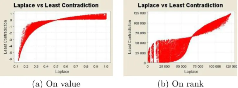
6.5 Distribution of interestingness values . . . 77

6.6 Joint-distribution matrix . . . 78

6.7 Correlation analysis . . . 79

6.8 Interesting rule analysis . . . 80

6.9 Ranking measures by sensitivity values . . . 81

6.9.1 On a ruleset . . . 81

6.9.2 On a set of rulesets . . . 82

6.10 Summary . . . 82

7 Comparative studies 85 7.1 Graph of stable clusters . . . 85

7.2 Comparative analysis: Pearson’s coefficient . . . 86

7.2.1 Discussion . . . 86

7.2.2 CG+ and CG0 . . . . 86

7.2.3 CG0 graphs: uncorrelated stability . . . . 86

7.2.4 CG+ graph: correlated stability . . . . 87

7.3 Comparative analysis: Spearman’s coefficient . . . 89

7.3.1 Discussion . . . 89

7.3.2 CG+ and CG0 . . . . 89

7.3.3 CG0 graphs: uncorrelated stability . . . . 91 vii

7.3.4 CG+ graph: correlated stability . . . . 91

7.4 Comparative analysis: Kendall’s coefficient . . . 92

7.4.1 Discussion . . . 93

7.4.2 CG+ and CG0 . . . . 94

7.4.3 CG0 graphs: uncorrelated stability . . . . 94

7.4.4 CG+ graph: correlated stability . . . . 95

7.5 Comparative analysis: all coefficients . . . 95

7.5.1 Discussion . . . 96

7.5.2 CG0 graphs: uncorrelated stability . . . . 96

7.5.3 CG+ graph: correlated stability . . . . 96

7.6 Comparative analysis: with AHC and PAM . . . 97

7.6.1 On a ruleset . . . 97

7.6.2 On two opposite rulesets . . . 98

7.7 Summary . . . 100

8 Conclusions and perspectives 108 8.1 Main results . . . 108 8.1.1 ARQAT tool . . . 109 8.1.2 Correlation graph . . . 110 8.1.3 Representative measure . . . 110 8.1.4 Comparison study . . . 110 8.1.5 Cluster evaluation . . . 111 8.2 Perspectives . . . 111

8.2.1 Improving the sample model . . . 111

8.2.2 Improving the cluster evaluation . . . 111

8.2.3 Hierarchy view . . . 112

8.2.4 Aggregation technique . . . 112

8.3 Publication . . . 112

Bibliography 114

2.1 A normalized database of sale transactions. . . 9

2.2 Binary representation of transactions. . . 10

2.3 Ordering items with support count (minsup = 2). . . . 17

2.4 Mining frequent itemsets with conditional FP-tree. . . 18

3.1 A list of objective measures. . . 28

3.2 Some matched properties of objective measures (Ind.: Independency, Equ.: Equi-librium, Sym.: Symmetry, Var.: Variation, Des.: Descriptive, Sta.: Statistical. < • >: matched, < ◦ >: unmatched). . . . 29

3.3 A classification of objective measures. . . 30

3.4 Some relations between objective measures . . . 30

4.1 Maximum entropy induced. . . 37

4.2 Rule structure for exceptions. . . 37

4.3 Rule classifications with a subjective measure. . . 40

4.4 An example of average ranking. . . 41

4.5 Dissimilarity values for three interestingness measures and five association rules. . . 48

4.6 Clusters of the measures obtained with PAM. . . 51

4.7 The supplementary information obtained on the clusters of a ruleset. . . 52

4.8 Correlation values for three measures and five association rules. . . 52

5.1 Characteristic types (remind that nXY = nX− nXY). . . 58

5.2 Frequency and inverse-cumulative in bins. . . 59

5.3 Some statistical indicators on a measure m. . . . 59

5.4 Sensitivity structure. . . 60

5.5 Average structure to evaluate sensitivity on a set of rulesets. . . 60

5.6 Matrix of correlation values. . . 62

5.7 Pearson’s values for three measures and five association rules. . . 62 ix

5.8 Spearman’s values for three measures and five rules. . . 63

5.9 Kendall’s values for three measures and five rules. . . 64

5.10 An example of concordant and discordant between the pairs of interestingness values computed from two objective measures m1 and m2 (< • >: concordant, < ◦ >: discordant). . . 64

6.1 Dataset description. . . 74

6.2 Rulesets extracted. . . 75

6.3 Trends on interestingness values . . . 78

7.1 Comparison of correlations with Pearson’s coefficient. . . 86

7.2 Comparison of correlations with Spearman’s coefficient. . . 92

7.3 Comparison of correlations with Kendall’s coefficient. . . 98

7.4 Comparison of correlation with all coefficients on the R1 ruleset. . . 101

7.5 Clusters of measures with AHC on R1 (dissimilarity interval = 0.15). . . 102

7.6 Clusters of measures with PAM on the R1 ruleset. . . 104

7.7 Clusters agreed with both AHC and PAM on the R1 ruleset. . . 105

7.8 Clusters of measures with AHC (measures are represented by their orders). . . 105

7.9 Cluster comparison from AHC (measures are represented by their orders). . . 106

7.10 Clusters of measures with PAM (measures are represented by their orders). . . 106

7.11 Cluster comparison from PAM (measures are represented by their orders). . . 107

7.12 Clusters agreed with both AHC and PAM on the R1, R01, R2, and R02 rulesets. . . 107

1.1 The steps in a KDD process. . . 2

1.2 Postprocessing models. . . 5

2.1 Lattice structure. . . 11

2.2 An example of finding all frequent itemsets with three database passes. . . 13

2.3 An FP-tree constituted from a set of transactions. . . 17

2.4 Lexicographic tree. . . 18

2.5 P-tree in the form of Rymon’s set enumeration tree. . . 19

2.6 Quantitative and categorical items. . . 19

2.7 Mapping to the boolean problem. . . 20

2.8 A taxonomy of items. . . 20

2.9 Adding taxonomy items to find frequent itemsets. . . 20

3.1 The cardinalities of a rule X → Y and the ”surprisingness” of negative examples. . . 23

4.1 Rymon’s set-enumeration tree for U = {A, B, C, D}. . . . 32

4.2 Fragment of an action tree for the supermarket management. . . 33

4.3 An AND-OR taxonomy. . . 34

4.4 IPS in the interestingness process. . . 34

4.5 Softness interval. . . 36

4.6 Ranking subset of contingency tables. . . 39

4.7 The profile building process. . . 39

4.8 A fragment of the template specification language. . . 40

4.9 The leaf level of the M-Tree. . . 41

4.10 The process of finding DS rules. . . 42

4.11 Interesting rules with r-neighborhood. . . 43

4.12 Overlapping of an attribute. . . 44

4.13 An attribute hierarchy. . . 45 xi

4.14 RuleVisualizer prototype. . . 46

4.15 The neighborhood relation for rummaging. . . 47

4.16 Visualization with the ARVis platform. . . 47

4.17 Clusters of measures with AHC on a ruleset. . . 49

4.18 Measures and clusters projected on the two principal axes of a PCA. The measures are presented by the symbols and the clusters are represented by the numbers. . . . 50

4.19 An illustration of the correlation graph. . . 51

5.1 ARQAT structure. . . 54

5.2 ARQAT modules. . . 55

5.3 Preprocessing of rulesets. . . 55

5.4 The filtering module. . . 56

5.5 The calculation module. . . 56

5.6 The sampling module. . . 57

5.7 Evaluating some characteristics of a ruleset. . . 58

5.8 Frequency and inverse-cumulative histograms of the Lift measure. . . 59

5.9 Drawing scatterplot view. . . 61

5.10 An example of two scatterplots on the ruleset Mushroom. . . 61

5.11 Computing correlation values. . . 62

5.12 An example of a line chart on Mushroom ruleset. . . 65

5.13 Summary scheme. . . 65

5.14 A summary structure (P: Pearson, S: Spearman, K: Kendall). . . 65

5.15 Stable combinations with correlation values (P: Pearson, S: Spearman, K: Kendall). 66 5.16 Summary scheme extracted from a ruleset (A lighter color box shows a τ -cluster, the otherwise a black box is a θ-cluster). . . . 66

5.17 Clustering measures. . . 67

5.18 Combination of cluster type for a cell in a matrix ([b] and [c] are only visualized for τ -cluster but it is the same for θ-cluster). [a] is visualized for the matrix with only one coefficient such as P, S or K. [b] is visualized for the matrix with two coefficients PS, PK or SK. [c] is visualized for the matrix with three coefficients PSK. . . 67

5.19 A process to compute a sample. . . 68

5.20 A stable hierarchy on a set of rulesets. . . 69

5.21 A summary computed from all the rulesets (original and sample). . . 69

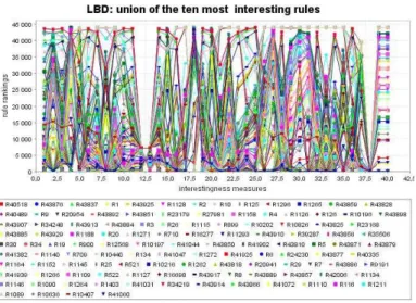
5.22 Union of the ten most interesting rules from all the measures on the LBD ruleset. . . 71

5.23 ARQAT Display. . . 71

5.24 Principal menu (extracted). . . 72

6.2 Characteristics of the rulesets (cont.). . . 77

6.3 Variation of the measure IPEE on the R1 ruleset. . . 77

6.4 Distribution of some measures on the R1 ruleset (extracted). . . 78

6.5 Some agreement and disagreement shapes. . . 79

6.6 Scatterplot matrix of joint-distributions on the R1 ruleset (extracted). . . 80

6.7 Coefficient matrix on the R1 ruleset. . . 81

6.8 CG0 and CG+ graphs on the R1 ruleset (clusters are highlighted with a gray back-ground). . . 82

6.9 Union of the ten most interesting rules for each measure of cluster C1 on the R1 ruleset (extracted). . . 83

6.10 Plot of the union of the ten most interesting rules for each measure of cluster C1 on the R1 ruleset. . . 83

6.11 Sensitivity rank on the R1 ruleset (extracted). . . 84

6.12 Comparison of sensitivity values on a couple of measures of the R1 ruleset. . . 84

6.13 Sensitivity rank on all the original rulesets (extracted). . . 84

7.1 τ -cluster on R1with Pearson’s coefficient. . . 87

7.2 CG+ graphs with Pearson’s coefficient. . . 88

7.3 CG+ graphs with Pearson’s coefficient (cont.). . . 89

7.4 CG0 graphs with Pearson’s coefficient. . . 90

7.5 CG0 graphs with Pearson’s coefficient (cont.). . . 91

7.6 CG+ graph with Pearson’s coefficient. . . . 92

7.7 τ -cluster on R1with Spearman’s coefficient. . . 93

7.8 CG+ graphs with Spearman’s coefficient. . . 94

7.9 CG+ graphs with Spearman’s coefficient (cont.). . . 95

7.10 CG0 graphs with Spearman’s coefficient. . . 96

7.11 CG0 graphs with Spearman’s coefficient (cont.). . . 97

7.12 CG+ graph with Spearman’s coefficient. . . . 98

7.13 τ -cluster on R1with Kendall’s coefficient. . . 99

7.14 CG+ graphs with Kendall’s coefficient. . . 100

7.15 CG+ graphs with Kendall’s coefficient (cont.). . . 101

7.16 CG0 graphs with Kendall’s coefficient. . . 102

7.17 CG0 graphs with Kendall’s coefficient (cont.). . . 103

7.18 CG+ graph with Kendall’s coefficient. . . 103 7.19 CG+ graphs with PS, PK, SK and PSK summaries on R1. . . 104

Introduction

This work takes place in the framework of knowledge discovery in databases (KDD), often called data mining. In the context of KDD, the extraction of rules in forms of association rules is a technique that is used frequently. The technique has the advantages to offer a simple model and unsupervised algorithms but it delivers a huge number of rules. So it is necessary to implement a postprocessing step to help the user to reduce the number of rules discovered.

One of the most attractive area in the knowledge discovery research is the automatic analysis of changes and deviation [PSM94] or the development of good measures of interestingness of discovered patterns [ST96]. As the number of discovered rules increases, end-users, such as data analysts and decision makers, are frequently confronted with a major challenge: how to validate and select the most interesting ones of those rules. More precisely, we are interested in the postprocessing of association rules with a set of interestingness measures. The main goal of our work relies on studying the behavior – theoretical and experiment – of interestingness measures for association rules.

1.1

The KDD process

Knowledge Discovery in Databases (KDD) is a research framework first introduced by Frawley et

al. [FPSM91]. A general definition of KDD is given in [FPSS96]: ”KDD is the nontrivial process

of identifying valid, novel, potentially useful, and ultimately understandable patterns in data”. The KDD process is well examined in the literature [BA96] [FPSS96] [HMS01]. Interaction and iteration in many steps with user’s decisions are the principal features of the process. The KDD process is illustrated in Fig. 1.1 [FPSS96]. The user interacts with the process by making decisions. The process operates on the following basic steps: (i) identifying the goal from the user’s point of view – based on the relevant knowledge about the domain –, (ii) creating a target data, (iii) data preprocessing, (iv) data reduction and projection, (v) matching the goals of the KDD process, (vi) exploratory analysis, (vii) data mining, (viii) interpreting mined patterns, (ix) acting on the discovered knowledge. These steps can be divided into three tasks: the preprocessing of data (steps i → vi), the mining of data (steps vii) and the postprocessing of data (steps viii → ix). The principal notions of the KDD process can be found in [KZ96].

The domain knowledge or background knowledge is the supplementary knowledge on the form, the data content, the data domain, the special situations and the process goal. The domain knowl-edge helps the process to focus on the research content. Most of the knowlknowl-edge comes from the domain expert. The basic knowledge contains the information on the knowledge that is already

2

Figure 1.1: The steps in a KDD process.

saved in the system. A dictionary1_{, a taxonomy, or a constraint of domain knowledge is an example} of this kind of knowledge [KZ02]. The structures such as decision tree or rules are used frequently. The procedures to extract the knowledge from data are called the discovery algorithms. Contingency tables, subgroup patterns, rules, decision trees, functional relations, clusters, taxonomies and con-cept hierarchies, probabilistic, causal networks, and neural networks are some forms of knowledge (i.e. pattern) [KZ02].

1.1.1

KDD system

A system implementing the steps of the KDD process is considered as a Knowledge Discovery System (KDS). It finds the knowledge that it has not before implicitly in its algorithms or explicitly in its domain knowledge. In this case, a knowledge (i.e. interesting and utility) is a relation or a pattern in the data [FPSM91]. A KDS includes a collection of components to identify or to extract the new patterns from the real data [MCPS93]. Interest and utility are considered as two important aspects. The components in a KDS can differ from each others but we can determine some principle functions such as the control, the data interface, the focus, the pattern extraction, the evaluation and the knowledge base. The control function manages the user’s demands and the parameters of other components. The data interface creates the questions on the data and then treats them. The

focus determines what portion of the data to analyze. The pattern extraction collects the algorithms

to extract the patterns. The evaluation evaluates the interests and utilities of extracted patterns. The knowledge base stores the specific information about the domain.

1.1.2

Who is the user?

Application is the final goal of any KDS. This application is used in a society, a company, etc. to supply the recommended analysis and actions. Its users can be a commercial person to see the important events in the business [BA96] (e.g. a decider, a decision-maker, a manager). A data analyst searches exploratory the basic tendencies or the patterns in a domain can become a user.

1.1.3

Postprocessing of association rules

In the framework of data mining [FPSS96], association rules [AIS93a] are a key tool aiming at dis-covering interesting implicative patterns in data. Since the precursor works about finding interesting patterns [PS91] [AIS93b] [AS94] in knowledge discovery in databases, the validation of association rules [AIS93a] [AMS+_{96] still remains a research challenge.}

Association rules

Association rule is one of the most important forms to represent the discovered knowledge in the mining task [AIS93a] [AS94] [AMS+_{96]. The first representation is of the form X}

1∧ X2∧ ...Xk → Y1 in which the antecedent is composed of many elements and the consequence is of only one element. Each element in the antecedent or consequent represents an item in a dataset. The transactions containing the bought items of the clients (e.g. in a supermarket) are often used as the datasets to analyze. The standard form X1∧ X2∧ ... ∧ Xk→ Y1∧ Y2∧ ... ∧ Ylis well developed with the Apriori

algorithm [AS94] [AMS+_{96]. In this form, both of the two parts of a rule (i.e. the antecedent and} the consequence) are composed with many items (i.e. a set of items or itemset), taking an important role in KDD.

Measures of interestingness

To evaluate the patterns issued from the second task (the mining task) [Sec. 1.1], the notion of interestingness is introduced [PSM94]. The patterns are transformed in value by interestingness measures. The interestingness value of a pattern can be determined explicitly or implicitly in a KDS. The patterns may have different ranks because their ranks depend strongly on the choice of interestingness measure. The interestingness measures are classified into two categories [ST96]: sub-jective measures and obsub-jective measures. The subsub-jective measures rely on the goals, the knowledge, and the belief of the user [PT98] [LHML99]. The objective measures are statistical indexes [AIS93a] [BA99] [BGGB05a] [BGGB05b]. The properties of the objective measures are briefly studied in [PS91] [MM95] [BA99] [HH01] [TKS04] [GCB+_{04] [Fre99] [Gui04] [VLL04].}

In the literature, many surveys deal with the interestingness measures according to two different aspects : the definition of a set of principles to select a suitable interestingness measure, and their comparison with theoretic criteria or experiments on data.

In the perspective to establish the principles of a best interestingness measure, Piatetsky-Shapiro [PS91] presented a new interestingness measure, called Rule-Interest (RI), and proposed three fun-damental principles for a measure on a rule X → Y : RI = 0 when X and Y are independent, RI monotonically increases with X ∧ Y , RI monotonically decreases with X or Y . Hilderman and Hamilton [HH01] proposed five principles : minimum value, maximum value, skewness, permutation invariance, transfer. Tan et al. [TKS02] [TKS04] defined five interestingness principles : symme-try under variable permutation, row/column scaling invariance, anti-symmesymme-try under row/column permutation, inversion invariance, null invariance. Freitas [Fre99] proposed an ”attribute surpris-ing” principle. Gras et al. [GCB+_{04] [Gui04] proposed a set of ten criteria to design a good} interestingness measure.

Among these reviews, some examine the comparison of the interestingness measures from their classification.

- Bayardo and Agrawal [BA99] concluded that the best rules according to all the interestingness measures must reside along a support/confidence border.

- Kononenco [Kon95] analyzed the biases of eleven measures for estimating the quality of multi-valued attributes and showed that the values of information gain, j-measure, gini-index, and relevance tend to linearly increase with the number of values of an attribute.

- Gavrilov et al. [GAIM00] studied the similarity between the measures for classifying them. - Hilderman and Hamilton [HH01] proposed five principles for ranking summaries generated from

databases by using sixteen diversity measures and illustrate that : (1) six measures satisfied the five principles proposed, (2) nine remaining measures satisfied at least one principle.

4

- By studying twenty-one measures, Tan et al. [TKS02] [TKS04] showed that none of the measures is adapted with all the cases and that the correlation of measures increases when support decreases.

- By using a method of multi-criteria decision-making aid integrating eight criteria, Vaillant et al. [VLL04] [LMP+_{04] extracted a pre-order on twenty measures and identify four clusters of} measures.

- Carvalho et al. [CFE05] [CFE03] evaluated eleven objective interestingness measures in order to rank them according to their effective interest for a decision maker.

- Choi et al. [CAK05] used an approach of multi-criteria decision-making to find the best association rules.

- Blanchard et al. [BGGB05a] [BGGB05b] classified eighteen objective measures into four clus-ters according to three criteria : independence, equilibrium, and descriptive or statistical characteristics.

- Huynh et al. [HGB05b] proposed a clustering approach by correlation graph which allows to identify eleven clusters on thirty-four interestingness measures.

Finally, two experimental tools are available : HERBS [VPL03] and ARQAT [HGB05a]. Postprocessing

Although the association rule model has the advantage of allowing an unsupervised extraction of rules and of illustrating implicative tendency in data, it has the disadvantage of producing a prohibitive number of rules. The final stage of the rule validation will let the user facing a main difficulty: how he/she can extract the most interesting rules among the large amount of discovered rules.

It is necessary to help the user in his/her validation task by implementing a preliminary stage of postprocessing of discovered rules. The postprocessing task aims at reducing the amount of rules by preselecting a reduced number of rules potentially interesting for the user. This task must take into account both his/her preferences and the data structure.

To solve this problem, five complementary postprocessing approaches are proposed in the liter-ature: constraints, pruning, grouping, summarizing, and visualizing. The first approach considers the whole set of rules as a database on which the user can extract the subsets of rules by requesting some integrated constraints [BBJ00] [SVA97] [WHP06]. The second one allows a significant re-duction by pruning the redundant or uninteresting rules [LGB04] [TKR+_{95] [BKGG03] [BGGB05a]} [BGGB05b]. The third one finds a special subset of rules that represents the underlying relationships [LHM99] [LHH00]. The fourth one groups the rules having the same properties into a meta-rule (e.g. a cover) that is more understandable [TKR+_{95] [DL98]. The last one uses graphical representations} to improve the readability of the results [BGB03b].

Since the introduction of support and confidence measures [AS94], many interestingness measures have been proposed in the literature [BA99] [HH01] [TKS04]. This abundance of interestingness measures leads to a second problem: how to help the user to choose the interestingness measures that are the best adapted to its goals and its data, in order to detect the most interesting rules.

We proposed a data-analysis technique for calculating the most suitable objective interestingness measures on a ruleset or a set of rulesets. For this purpose, some clustering techniques such as AHC [KR90], PAM [KR90] or correlation graph [HGB06d] are used with the correlation values, in order to partition a set of interestingness measures into kc clusters. The subset of representative measures

1.2

Postprocessing models

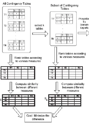
Together with the huge patterns discovered by the KDS at the mining step, there are many models have been proposed to evaluate the discovered patterns [ST95] [LHML99] and to identify the most interesting ones [ST96]. Fig. 1.2 [ST95] [LHML99] shows the four main models that are widely used in the literature. In Fig. 1.2 (a), the patterns mined by the KDS are immediately considered as the most interesting ones. In Fig. 1.2 (b), the uninteresting patterns are filtered out by an interestingness filter. In Fig. 1.2 (c), the KDS interacts with an interestingness engine. The last model in Fig. 1.2 (d) [LHML99] uses a post-analysis component IAS (Interestingness Analysis System) to help the user identify interesting patterns.

Figure 1.2: Postprocessing models.

The fist model (a) in these four main models is the simplest approach. The KDS outputs the patterns directly to the user. The user can not interact with the KDS because the KDS works independently. When the KDS delivers a considerable number of patterns, it is difficult to the user to realize which ones are the interesting or uninteresting to learn about. The second model (b) depends on the efficiency of the interestingness filter. A lot of number of uninteresting patterns can be cut out by the interestingness filter but like the first model, no user interaction that are integrated into the filter process. The third model (c) is more flexible than the two previous models (a) and (b). It implements an interestingness engine to communicate with the KDS. The domain knowledge can be used efficiently in this model and many users can interact separately or parallel to determine his/her own interests. The fourth model (d) evaluates the patterns issued from the KDS by an independent system. The system includes several tools to rank the patterns with user’s interactions. One important feature of the last model is that it allows to use interestingness measures to examine the patterns. Each tool can work independently.

1.3

Clustering techniques

Clustering aims at finding the similar elements in data and to group them into the same group or cluster [KR90] [DHS01]. The number of cluster has to be predetermined [HBV01] [KR90]. The notion of similarity can be understood according to the domain knowledge, the context or the user’s point of view. The clustering process is used with no prior knowledge so it is also called unsupervised leaning.

The clustering methods can be divided into 4 groups [JMF99] [HBV01] such as partitioning clustering, hierarchical clustering, density-based clustering and grid-based clustering. Partitioning

6

clustering and hierarchical clustering are two methods that are used frequently. The datasets can be available in one of the following matrices [KR90]:

- an q × p attribute-value matrix. Columns are attributes and rows are the values of each elements according to the corresponding attributes,

- an q × q dissimilarity matrix. In this matrix, the difference between each pair of attributes are calculated. This value is considered as a dissimilarity value or a distance value. Noted that d(i, j) = d(j, i) and d(i, i) = 0 where d(, ) is the dissimilarity or distance between any two attributes i and j.

In the following, we will describe the two techniques that are used in our work.

1.3.1

Partitioning clustering

The elements in a dataset is divided into kc clusters. The number of clusters kc is given by the

user. How we can determine the ”best” partition with a value of kc is always an attractive

prob-lem [HBV01] [Sap90]. The best partition depends on the point of views of the user or it can be determined automatically by a ”quality index”. Some methods in this clustering type are PAM (Par-titioning Around Medoids) – more robust than the k-means [McQ67] –, CLARA (Clustering Large Applications), CLARANS (Clustering Large Application Based on Randomized Search) [KR90].

1.3.2

Hierarchical clustering

The elements in a dataset is firstly grouped into small clusters. These small clusters are then merged into bigger ones. The result is represented by a tree called dendrogram [KR90]. The method that uses the small clusters to merge into bigger clusters is called agglomerative method (i.e. Agglomerative Hierarchical Clustering – AHC). Inversely, the method that processes, from bigger cluster into smaller cluster, is called divisive method.

1.4

Thesis contribution

In recent years, the problem of finding interestingness measures to evaluate association rules has become an important issue in the postprocessing stage in KDD. Many interestingness measures may be found in the literature, and many authors have discussed and compared interestingness properties in order to improve the choice of the most suitable measures for a given application. As interestingness depends both on the data structure and on the decision-maker’s goals, some measures may be relevant in some context, but not in others. Therefore, it is necessary to design new contextual approaches in order to help the decision-maker select the most suitable interestingness measures and as a final goal, select the most interesting association rules.

In our thesis, we focus on the interestingness measures technique in the pruning approach, espe-cially on the objective interestingness measures. Postprocessing of association rules with interest-ingness measures is our main research. Our thesis contributions are:

• A dedicated ARQAT tool (Association Rule Quality Analysis Tool) for the postprocessing of

association rules [HGB05a]. ARQAT is used to study the specific behavior of a set of interest-ingness measures in the context of specific datasets and in an exploratory analysis perspective. More precisely, ARQAT is a toolbox designed to help a data-analyst to capture the most suitable measures and as a final purpose, the most interesting rules within a specific ruleset.

Similarly with the model (d) in Fig. 1.2, ARQAT tool has some strong features in comparison with IAS tool: (i) allows ranking the discovered patterns with a set of interestingness mea-sures, (ii) easily determines the most interesting patterns with complementary views, (iii) the comparisons can be drawn on many datasets.

• A representative measure approach, especially with correlation graph (CG),

agglom-erative hierarchical clustering (AHC), and partitioning around medoids (PAM) techniques. This approach reflects the postprocessing of association rules, implemented by the ARQAT tool2_{. The approach is based on the analysis the dissimilarities computed from interestingness} measures on the data to find the most suitable measures.

• A comparative study on the stable clusters between interestingness measures. The result is

used to compare and discuss the behavior of 40 interestingness measures on two prototypical and opposite datasets (i.e. a correlated one and a weakly correlated one) and on other two real-life datasets. We focus on the discovery of the stable clusters obtained from the data analyzed between these 40 measures, showing unexpected stabilities.

1.5

Thesis structure

The remaining of the document is structured in seven chapters as follows.

In the first chapter, the association rules discovery process is introduced. We start from the prob-lem of basket market transactions to the association approach with binary representation. Finding frequent itemsets as well as generating rules with anti-monotonicity property is also examined. We classify the improvements from the Apriori algorithm into five principal groups: database pass, computation, itemset compaction, search space and data type.

Chapter 3 gives an overview on the measures of interestingness with two types: subjective mea-sures and objective meamea-sures. Two important aspects of the subjective meamea-sures such as actionability and unexpectedness are introduced. In this chapter, we analyze an association rule X → Y objec-tively by a function f (n, nX, nY, nXY) with four parameters. We also conduct a detail survey on

several important properties of an objective measure studied in the literature. As a result, this sur-vey gives us a classification of 40 objective measures. Some mathematical relations between these objective measures are also given in this chapter.

Chapter 4 examines five principal approaches in the postprocessing step of association rules that are well studied in the literature: constraints, pruning, summarization, grouping and visualizing. We proposed our new technique representative measures as a pruning approach. This new technique uses AHC, PAM or correlation graph as a means to achieve the most interesting rules.

Chapter 5 represents the ARQAT tool, a new tool for the postprocessing step of association rules written in Java. The tool provides five principal tasks with 14 views. The tool is structured into three analyzed phases: preprocessing, evaluation and display.

Chapter 6 analyzes some principal opposite types of rulesets: correlated vs weakly correlated, real-life vs synthetic. To have a general analysis on these rulesets, we extracted a sample rulesets from each original rulesets. The sample rulesets contains only the most interesting rules due to some objective measures. We also introduce couple and multiple as two abstract types of rulesets. The couple rulesets is used to evaluate the behaviors on objective measures on an original ruleset with its sample ruleset. The multiple ruleset is used to evaluate on many rulesets. These two types of rulesets are also named commonly as complement ruleset. This chapter gives some results on evaluating the

8

efficiency of the sample models, distributions of interestingness values, joint-distribution matrix, correlation analysis, interesting rules analysis, and ranking of measures by sensitivity values.

Chapter 7 examines the stable clusters of measures between 40 objective measures on three well-known correlation coefficients: Pearson, Spearman and Kendall. A comparative study on the stable behaviors of measures in a rulesets over all these three coefficients is also evaluated.

Finally, chapter 8 gives a summarization of our thesis contribution on the postprocessing step in a KDD process with association rules. We open some future research topics such as improving the sample model, improving the cluster evaluation, hierarchy view, and the aggregated measures by Choquet’s or Sugeno’s integral.

Discovery of association rules

Discovering association rules between items in large databases is a frequent task in KDD. The purpose of this task is to discover hidden relations between items of sale transactions. This later is also known as the market basket database1_{. An example of such a relation might be that 90% of} customers that purchase bread and butter also purchase milk [AIS93a].

2.1

From the data ...

We consider a database of sale transactions in Tab. 2.1 as a basket data. Each record in this database consists of items bought in a transaction. The problem is how we can find some interesting (i.e. hidden) relations existing between the items in these transactions or some interesting rules that a manager (a user, a decider or a decision-maker) who owns this database can take some valuable decisions. Some rules derived from this database can be {Wine} → {Cheese} or {Bread, Chocolate}

→ {Milk}.

To facilitate the process of finding the hidden relations mentioned above, the database can be normalized [AS94] [AMS+_{96]. For instance, the database in Tab. 2.1 is a normalized database} because all of its items in the four records are in lexicographic orders.

Tid Items

100 {Bread, Chocolate, Milk}

200 {Cheese, Chocolate, Wine}

300 {Bread, Cheese, Chocolate, Wine}

400 {Cheese, Wine}

Table 2.1: A normalized database of sale transactions.

Definition 2.1.1 (Normalized database [AS94] [AMS+_{96]). A database D is said normalized if} items in each record of D are kept sorted in their lexicographic order. Each database record is a

1_{In our work, the words database and dataset can be used interchangeable.}

10

transaction represented by a <Tid, item> pair. The transaction is determined by its transaction identifier Tid.

2.2

... To association approach

Association rules are rules of the form If X then Y with a percentage of trust (e.g., 2%, 5%, 90%, ...). The formal statement of the problem is given in [AMS+_{96]. Let I = {i}

1, i2, ..., im} be a set of

literals, called items. Let D be a set of transactions, where each transaction T is a set of items such that T ⊆ I. Associated with each transaction is a unique identifer, called its T ID. A set of items

X ⊂ I is called itemset. A transaction T is said contains X, if X ⊆ T . The approach presented in

this section is also known as the Apriori algorithm [AS94][AMS+_96].

Definition 2.2.1 (Association rule). An association rule is an implication of the form X → Y , where X ⊂ I, Y ⊂ I, and X ∩ Y = ∅.

More precisely [AMS+_{96], I = {i}

1, i2, ..., im} is set of attributes over the binary domain {0, 1}.

A tuple T of the database D is represented by identifying the attributes with value 1. We also called this approach is a binary association rule approach. An example of this transformation is given in Tab. 2.2.

TID Bread Cheese Chocolate Milk Wine

100 1 0 1 1 0

200 0 1 1 0 1

300 1 1 1 0 1

400 0 1 0 0 1

Table 2.2: Binary representation of transactions.

Definition 2.2.2 (Support). The rule X → Y has support s in the transaction set D if s% of transactions in D contain X ∪ Y .

Definition 2.2.3 (Confidence). The rule X → Y has confidence c if c% of transactions in D that contain X also contain Y .

The rule X → Y holds in the transaction set D with confidence c and support s. It will be retained when its support and confidence greater than the user-specified minimum support (minsup) and minimum confidence (minconf ).

The process of discovering all association is performed via two steps [AIS93a] [AS94] [AMS+_96]: (i) finding all frequent itemsets with minsup and minconf (all others are infrequent itemsets), (ii) generating rules with the frequent itemsets found.

(a)

(b) Monotonicity (c) Anti-monotonicity

Figure 2.1: Lattice structure.

2.2.1

Monotonicity

A lattice structure is proposed to hold the search space containing all the possibly combinatory cases between the items in the transaction set in the process of finding association rules. The use of this lattice structure leads to an combinatorial explosion of itemsets in the search space 2n_{, including the}

empty set, with n is the number of items. For example, for a search space of 5 items, the number of search elements is 25_{= 32. If we note the five items in Tab. 2.1 as A, B, C, D, and E for short, all} the combinations between the first four items in form of a lattice is represented in Fig. 2.1 (a).

To overcome the combinatory problem, the monotonicity (anti-monotonicity respectively) prop-erty is used to prune unnecessary cases efficiently.

Definition 2.2.4 (Monotonicity/Anti-monotonicity). If a set X has a property t then all its sub-sets/supersets also have the property t.

Reconsider the lattice constructed from four items {A, B, C, D} in Fig. 2.1 (a). If {A, B, C} are in grey then all its subsets {AB, AC, BC, ABC} are in grey with the monotonicity property (see Fig. 2.1 (b)). For the anti-monotonicity property (see Fig. 2.1 (c)), if {A, B} are in grey then all its supersets {AB, AC, AD, BC, BD, ABC, ABD, ACD, BCD, ABCD} are also in grey.

2.2.2

Frequent itemsets

The itemsets that have transaction support above minsup are called frequent itemsets2_{. A k-itemset} is an itemset has itself k items. To discover frequent itemsets, multiple passes over the database are

2_{The term frequent itemset is also known as large or covering itemset in [AS94] [AMS}+_{96]. Infrequent itemset is}

12

performed. Firstly, the support of each item is counted and the item type (frequent/infrequent) is determined by using minsup value.

Candidate itemsets

In the next passes, the frequent itemsets discovered in the previous pass is held as a seed set to generate new potentially frequent itemsets or candidate itemsets using the monotonicity property. The support counts for these candidate itemsets are also determined during this process. Among these candidate itemsets at the end of a database pass, those ones have the support count above the

minsup threshold are held, the others are cut by using the anti-monotonicity property. The process

will finish when no new frequent itemsets appear. Algorithm

Let Lk be the set of frequent k-itemsets. Let Ck be the set of candidate k-itemsets. The algorithm

to find all frequent itemsets can be represented as follows [AMS+_96]. Algorithm FindFrequentItemset

L1 = frequent 1-itemsets;

for (k = 2; Lk−16= ∅; k++) do begin

Ck= apriori-gen(Lk−1);

forall transactions t ∈ D do begin

Ct = subset(Ck, t); forall candidates c ∈ Ct do c.count++; end; Lk= c ∈ Ck|c.count ≥ minsup end returnS_kLk

The apriori-gen function returns a superset of the set of all frequent (k − 1)-itemsets from the previous pass Lk−1. It works in two steps: (i) joints Lk−1 with Lk−1 and (ii) prunes all itemsets c ∈ Ck in which (k-1)-subset of c is not in Lk−1. For instance, let L3be {ABC, ABD, ACD, ACE, BCD}. The candidate C4 will be {ABCD, ACDE}. Because the itemset {ADE} is not in L3so the itemset {ACDE} will be deleted and only the itemset {ABCD} exists in C4. Fig. 2.2 illustrates a complete example with three database passes for the transactions in Tab. 2.1.

2.2.3

Rule generation

The rule generated in this process has the form X → Y in which X and Y are two itemsets, |X| > 0,

|Y | > 0, support(X∪Y )_support(X) ≥ minconf [AS94] [AMS+_{96]. X and Y are called the antecedent and the} consequent of the rule X → Y respectively. Given a frequent itemset L, all the rules X → (L − X) are outputted where X ⊆ L and the previous conditions are held. The RuleGeneration algorithm creates firstly all the rules with one item in the consequent. The consequents of these rules are used as a seed set (as the function apriori-gen in Sec. 2.2.2) to generate all the rules with two items in the consequent and so on.

Database D TID Items 100 A C D 200 B C E 300 A B C E 400 B E Counting −−−−−−→ C1 Itemset Support {A} 2 {B} 3 {C} 3 {D} 1 {E} 3 Pruning −−−−−→ L1 Itemset Support {A} 2 {B} 3 {C} 3 {E} 3 C2 Itemset {A B} {A C} {A E} {B C} {B E} {C E} Counting −−−−−−→ C2 Itemset Support {A B} 1 {A C} 2 {A E} 1 {B C} 2 {B E} 3 {C E} 2 Pruning −−−−−→ L2 Itemset Support {A C} 2 {B C} 2 {B E} 3 {C E} 2 C3 Itemset {B C E} Counting −−−−−−→ C3 Itemset Support {B C E} 2 Pruning −−−−−→ L3 Itemset Support {B C E} 2

Figure 2.2: An example of finding all frequent itemsets with three database passes.

A remark for the RuleGeneration algorithm can be drawn. If the rule X → Y are held then all the rules X ∪ (Y − Y0_{) → Y}0 _{are also held where Y}0 _{⊆ Y . For example, if the rule AB → CD is}

held, then the other rules such as ABC → D and ABD → C are also held. D in ABC → D and C in ABD → C hold the role of Y0 _{respectively.}

2.3

Algorithm improvement

The volume of association rules tends to be huge and the time execution to be expensive. To improve the efficiency of finding association rules, several strategies are proposed. We classify these strategies into five subgroups: database pass, computation, itemset compaction, search space and data type. Excellent surveys can be found in [CHY96] [ZB03] [TSK06] [CR06] [Zak99].

2.3.1

Database pass

The principal Apriori algorithm requires multiple passes over the database: for finding the candi-dates of k-itemsets, k passes are executed (see Fig. 2.2). The approaches proposed in this strategy aims at reducing a significance number of scans, performing efficiently in I/O times.

Partition

Partition [SON95] uses at most two passes on the database. It generates a set of all potentially frequent itemsets in the first scan. The counters for each of the itemsets are set up, together with their actual support is measured, in the second one.

14

Algorithm RuleGeneration

forall large k-itemsets lk, k ≥ 2 do begin

H1 = {consequents of rules from lk with one item in the consequent}

call ap-genrules(lk, H1);

end

procedure ap-genrules(lk: large k-itemset, Hm: set of m-item consequents)

if (k < m + 1) then begin

Hm+1= apriori-gen(Hm);

forall hm+1∈ Hm+1do begin

conf = support(lk)/support(lk− hm+1);

if (conf ≥ minconf) then

output the rule (lk− hm+1→ hm+1)

with confidence = conf and support = support(lk)

else

delete hm+1from Hm+1

end

call ap-genrules(lk, Hm+1);

end

The database in the first step is divided into a number of non-overlapping partitions. Each partition is considered one at a time and all frequent itemsets for that partition are generated. Then, these frequent itemsets are merged to generate a set of all potentially frequent itemsets. The supports for these merged itemsets are generated and the frequent itemsets are identified in the second step. Each partition is read into the memory only one time according to its appropriate size. DIC

Dic [BMUT97] finds frequent itemsets with fewer database passes based on the idea of item reorder-ing. By keeping the number of itemsets which are counted in any pass, the number of passes is then reduced efficiently. It means that the support of an itemset can be counted whenever it may be necessary to count instead of waiting until the end of the previous pass. For instance, Apriori can produce 3 passes for counting 3-itemsets while Dic produces 1.5 passes. And in the first pass with 1-itemset, Dic can count some itemsets that are in 2-itemsets or 3-itemsets. Four possible states (confirmed frequent, confirmed infrequent, suspected frequent, suspected infrequent) for an itemset are used during the time that the itemsets are counted in one pass.

Sampling

Sampling [Toi96] can find association rules very efficiently in only one database pass and two passes in the worst case. A random sample S is picked and used to find frequent itemsets with the concept of negative border.

Let S be a set of itemsets. The border Bd(S) of S is defined as a set of itemsets such that all subsets of Bd(S) are in S and none of the supersets of Bd(S) is in S [MT96]. The positive border

Bd+_{(S) (the negative border Bd}−_{(S) respectively) contains the itemsets such that Bd}+_{(S) = {x|x ∈}

Bd(S), x ∈ S} (Bd−_{(S) = {x|x ∈ Bd(S), x 6∈ S} respectively). We have Bd(S) = Bd}+_{(S) ∪ Bd}−_(S)

B, C, AB, AC, BC, ABC}. In S, only ABC has all its supersets are not in S so Bd+_{(S) = {ABC}.} We can see the same situation with the negative border when only D has all its subsets are in S (e.g. {∅}) and D is not in S, so we have Bd−_{(S) = {D}. The border set of S can be established as} Bd(S) = Bd+_{(S) ∪ Bd}−_{(S) = {ABC} ∪ {D} = {D, ABC}.}

2.3.2

Computation

To resolve the problem of expensive cost of time calculations, some approaches based on the parallel and distributed techniques are proposed [AS96] [PCY95] [Zak99]. The task can be parallel with the whole or partitioned database. The database can be distributed across the multiprocessors. Overall, four techniques are introduced: (i) count distribution, (ii) data distribution, (iii) candidate distribution, and (iv) rule distribution.

Assuming a shared-nothing architecture with n processors in which each processor has a private memory and a private disk. The processors are connected by a communication network and can communicate only by passing messages. Data is distributed on the disks attached to the processors and the disk of each processor has approximately an equal number of transactions.

Count distribution

In this approach, the support counts for Lk in the pass k are distributed. Except the first pass

is special, from the second pass we have five tasks in each pass: (i) a processor Pi _{generates the}

complete Ck taking as argument the frequent itemset Lk−1of the pass k − 1. The same Ck will be

generated overall processors Pi _{because of the same L}

k−1, (ii) the local support for each candidate

is counted with a pass from the processor Pi _{on its data D}i_{, (iii) the global count for C} k are

determined by exchange with the local Ck counted by each processor Pi, (iv) Lk is computed from Ck in each processor Pi, (v) the continuation is depended on each processor Pi independently. The

most important feature of the count distribution is that no data are exchanged between processors except the counts.

Data distribution

This approach is used to better exploit the total memory in a system with n processors. The purpose is to count in a single pass a candidate set that would require n passes in the count distribution approach. So that every processor must broadcast its local data to all other processors in every pass. On a machine with very fast communication, this approach will work viable.

Candidate distribution

Each processor in this approach may proceed independently with both the data and the candidates partitioned. In a pass k, the algorithm divides the frequent itemset Lk−1between processors in such

a way that a processor Pi _{can generate a unique C}i

m (m ≥ k) independent of all other processors

(Ci

m∩ Cmj = ∅, i 6= j). Because the data is partitioned so that a processor can count candidates in Ci

16

Rule distribution

The above three techniques are about generating frequent itemsets. This technique is to generate rule by parallel implementation. By partitioning the set of all frequent itemsets into each processors, then the proportions of rules are generated conformably.

2.3.3

Frequent itemset compaction

Because of the combinatory cases between items in a set of transactions, the problem of compacting a lattice structure is introduced. Two useful representations of the frequent itemsets are frequent

closed itemsets and maximal frequent itemsets. We have the following relation between these three

sets: {maximal frequent itemsets} ⊆ {frequent closed itemsets} ⊆ {frequent itemsets}. Frequent closed itemsets

A closed itemset is a maximal set of items common to a restricted set of transactions [PBTL99]. It will be called a frequent closed itemset if its support count is greater or equal to minsup threshold. For instance, the database D in Tab. 2.1 or in Fig. 2.2 has the itemset BCE is a closed itemset because it satisfies the closed condition with two transactions TID=200 and TID=300. It is also a frequent closed itemset when its support count is 2 ≥ minsup. The useful meaning of this technique is that 50% of customers purchase at most three items Cheese, Chocolate, and Wine. The total set of frequent closed itemsets for the transactions in the database D is {AC, BE, C, BCE}.

The closed itemset lattice is often much smaller than the itemset lattice. By using a closure mechanism based on the Galois connection and two properties that (i) the support of an itemset T is equal to the support of its closure and (ii) the set of maximal frequent itemsets3 _{is identical to} the set of maximal frequent closed itemsets. With a reduced set of frequent closed itemsets instead of a larger frequent itemsets then the set of association rules can be reduced without the loss of information.

Maximal frequent itemset

A maximal frequent itemset [BCF+_{05] is a frequent itemset and all its superset are infrequent. This} technique is especially efficient when the itemsets are very long (more than 15 to 20 items). By using a cut through the lattice structures so all itemsets above the cut are frequent itemsets, and all their subsets below are infrequent. All the combinations above the cut (i.e. frequent itemsets) form the positive border when all the combinations below the cut (i.e. infrequent itemsets) form the negative border.

In Fig. 2.1 (b), if we consider all the nodes in grey are frequent and not in grey are infrequent, then only one itemset ABC is a maximal frequent itemsets because all its supersets are infrequent.

2.3.4

Search space

Due to the explosive combination of the candidate itemsets while searching the frequent itemsets, many authors have proposed some efficient search space techniques in which we can ignore the step of finding candidate itemsets and we can go directly to find the frequent itemsets. Most of them

3_{The meaning of maximal set in this case is used in a normal way. This is not understandable like the next}

are based on tree structures. We will present such three attractive structures: (i) FP-tree, (ii) lexicographic tree, and (iii) T-tree and P-tree.

FP-tree

FP-tree (Frequent-Pattern Tree) [HPYM04] is a tree structure for mining frequent itemsets efficiently without candidate generation. It is defined as: (i) one root labeled as ”null”, a set of item-prefix subtrees as the children of the root, and a frequent-item-header table (ii) each node of the item-prefix subtree consists of three fields: item-name, count, and node-link where item-name registers which item this node represents, count registers the number of transactions represented by the portion of the part reaching this node, and node-link links to the next node in the FP-tree carrying the same item-name, or null if there is none (iii) each entry in the frequent-item-header consists of two fields: (iii-1) item-name and (iii-2) head of node-link (a pointer pointing to the first node in the FP-tree carrying the item-name). For instance, in Fig. 2.3, an FP-tree is constituted from a set of transactions in Tab. 2.1, ordered by support count in Tab. 2.3.

TID Items bought (Ordered) frequent items

100 A C D C:3 A:2

200 B C E B:3 C:3 E:3

300 A B C E B:3 C:3 E:3 A:2

400 B E B:3 E:3

Table 2.3: Ordering items with support count (minsup = 2).

Figure 2.3: An FP-tree constituted from a set of transactions.

tree mines completely the set of frequent itemsets by itemset fragment growth. The FP-growth algorithm uses this tree to find frequent itemset efficiently with both long and short itemsets. It can be considered as an order of magnitude faster than the Apriori algorithm. Tab. 2.4 shows the conditional FP-tree constituted from the FP-tree in Fig. 2.3 for extracting frequent itemsets.

COFI-tree [EHZ03] and CATS-tree [CZ03] are two tree structures that are inspired from the FP-tree to reduce the memory space needed.

18

Item Conditional pattern-base Conditional FP-tree A {(C:1), (BCE:1)} {(C:2)}|A

E {(BC:2), (B:1)} {(B:3)}|E

C {(B:2)} {(B:2)}|C

B ∅ ∅

Table 2.4: Mining frequent itemsets with conditional FP-tree. Lexicographic tree

By constructing successively the nodes of a lexicographic tree of itemsets, the set of frequent item-sets are constituted [AAP01]. Fig. 2.4 show a lexicographic tree established from 5 items. The frequent itemsets are represented as nodes of the lexicographic tree to reduce the CPU time for counting frequent itemsets. The support counts of the frequent itemsets, in a top-down manner, are determined by projecting the transactions onto the nodes of the tree. It illustrates an advantage of visualizing itemset generation with the flexibility of picking the correct strategy during the tree generation phase as well as transaction projection phase.

The lexicographic tree is defined as: (i) a vertex exists in the tree corresponding to each frequent itemset (the root corresponds to the null itemset), (ii) let I = {i1, i2, ..., ik} be a frequent itemset,

where i1, i2, ..., ik are listed in lexicographic order and the parent of the node I is the itemset {i1, i2, ..., ik−1}. The levels in a lexicographic tree correspond the itemset sizes. The possible states

for a node are: generated, examined, null, active or inactive.

Figure 2.4: Lexicographic tree.

T-tree and P-tree

P-tree and T-tree that are two tree structures quite similarly for counting the support of itemsets based on Rymon’s set enumeration tree [CGL04]. T-tree (Total Support Tree) is implemented to reduce number of links needed and providing direct indexing. P-tree (Partial Support Tree) is used with the concept of partial support. Fig. 2.5 illustrates an example with 5 items {A, B, C, D, E}.

2.3.5

Data type

Due to the different types of data, many authors have conducted their researches to discovery as-sociation rules adapted to different data types such as quantitative and categorical [SA96], interval [MY97], spatial [KH95], temporal [CP00], ordinal [Gui02], multimedia [ZHZ00], text [AAFF05],

Figure 2.5: P-tree in the form of Rymon’s set enumeration tree.

multidimensional [LHF98], and taxonomy-based [SA95]. We will present in this part the two most important data types are recently developed and widely used: quantitative/categorical and taxonomy-based.

Quantitative and categorical

When an attribute (i.e. an item) is quantitative or categorical then boolean attributes can be considered a special case of categorical attributes [SA96]. Fig. 2.6 shows a People table with three non-key attributes: Age, NumCars (quantitative), and Married (categorical). A possible quantitative association rule is: < Age : 30..39 > and < M arried : Y es >→< N umCars : 2 >.

TID Age Married NumCars

100 23 No 1

200 25 Yes 1

300 29 No 0

400 34 Yes 2

500 38 Yes 2

Figure 2.6: Quantitative and categorical items.

Many fields as the number of attribute values are established instead of just one field in the table. For a quantitative attribute, its values will be partitioned into intervals and then map each

< attribute, interval > pair to a boolean attribute as in the boolean field. The number of intervals

can be calculated as: 2n

m(K−1) where n is the number of quantitative attributes, m is the minimum

support (as a fraction) and K is the partial completeness level (see how we can find K in [SA96]). Fig. 2.7 shows this mapping for the non-key attributes of the People table given in Fig. 2.6. Taxonomy-based

When there is a taxonomy on the items in the transactions of a database (see Fig. 2.8), the association rules can be generated for all levels (e.g. generalized – [SA95] or at different levels (e.g. multiple-level association rules – [HF99]). For example, a generalized association rule is an association rule X → Y that is no item in Y is an ancestor of any item in X. The reason for

20

TID Age:20..29 Age:30..39 Married:Yes Married:No NumCars:0 NumCars:1 NumCars:2

100 1 0 0 1 0 1 0

200 1 0 1 0 0 1 0

300 1 0 0 1 1 0 0

400 0 1 1 0 0 0 1

500 0 1 1 0 0 0 1

Figure 2.7: Mapping to the boolean problem.

the condition that no item in Y should be an ancestor of any item in X is that a rule of the form ”x → ancestor(x)” is trivially true with 100% confidence, and hence redundant. The rules are called generalized association rules because both X and Y can contain items from any level of the taxonomy, a possibility not entertained by the formalism introduced in [AIS93a].

Figure 2.8: A taxonomy of items.

Inspired from a similar example illustrated in [SA95], given a set of items {Cheese, Cow Milk, Emmental, Raclette, Ewe Milk, Roquefort, Bread, White Bread, Brown Bread}, Fig. 2.8 shows the corresponding taxonomy being composed of these items. Consider the set of transactions shown in Fig. 2.9 (a) with minsup = 2. Then the frequent itemsets corresponding to these itemsets are illustrated in Fig. 2.9 (b).

TID Items bought

100 Roquefort

200 Emmental, Brown Bread 300 Raclette, Brown Bread

400 White Bread

500 White Bread

600 Emmental

(a) D

Adding taxonomy items

−−−−−−−−−−−−−−−−−−→ Itemset Support {Emmental} 2 {Cow Milk} 3 {Cheese} 4 {White Bread} 2 {Brown Bread} 2 {Bread} 4

{Cow Milk, Brown Bread} 2

{Cheese, Brown Bread} 2

{Cow Milk, Bread} 2

{Cheese, Bread} 2

(b) Frequent itemsets Figure 2.9: Adding taxonomy items to find frequent itemsets.