HAL Id: tel-00789856
https://tel.archives-ouvertes.fr/tel-00789856
Submitted on 18 Feb 2013HAL is a multi-disciplinary open access archive for the deposit and dissemination of sci-entific research documents, whether they are pub-lished or not. The documents may come from teaching and research institutions in France or abroad, or from public or private research centers.
L’archive ouverte pluridisciplinaire HAL, est destinée au dépôt et à la diffusion de documents scientifiques de niveau recherche, publiés ou non, émanant des établissements d’enseignement et de recherche français ou étrangers, des laboratoires publics ou privés.
bipèdes
Ting Wang
To cite this version:
Ting Wang. Contribution à la commande de robots marcheurs bipèdes. Robotique [cs.RO]. Ecole Centrale de Nantes (ECN), 2011. Français. �tel-00789856�
ÉCOLE DOCTORALE SCIENCES ET TECHNOLOGIES
DE L’INFORMATION ET MATHÉMATIQUES
Année 2011 N˚attribué par la bibliothèque
F F F F F F F F F F
Contribution à la commande de robots
marcheurs bipèdes
THÈSE DE DOCTORAT
Discipline : Automatique et Informatique Appliquée Spécialité : Robotique
Présenté
et soutenue publiquement par
Ting WANG
Le 8 Décembre 2011, devant le jury ci dessous
Président
... ... ...
Rapporteurs
Mazen ALAMIR Directeur de Recherche, CNRS, à GIPSA-Lab
Olivier BRUNEAU Maître de Conférences à l’Université de Versailles Saint Quentin
Examinateurs
Gabriel ABBA Professeur à l’École Nationale d’Ingénieurs de Metz
Rodolphe GELIN Chef des projets collaboratifs à Aldebaran Robotics
Yannick AOUSTIN Maître de Conférences à l’Université de Nantes
Christine CHEVALLEREAU Directeur de Recherche, CNRS, à l’IRCCyN
Directeur de thèse : Christine CHEVALLEREAU
Introduction 1
1 Walking control of an under-actuated planar biped robot 7
1.1 Introduction . . . 7
1.2 Description of the studied robot . . . 8
1.2.1 Biped model. . . 8
1.2.2 Walking gait. . . 10
1.3 Dynamic model during different walking phases . . . 11
1.3.1 Lagrange formulation . . . 11
1.3.2 Swing phase model . . . 13
1.3.3 Impact model . . . 13
1.3.4 Hybrid model of walking . . . 16
1.4 A control law for tracking parametrized reference trajectory . . . 16
1.4.1 The reference trajectory . . . 17
1.4.2 Calculation of the input torques . . . 18
1.4.3 Stability analysis . . . 19
1.5 Two control laws for tracking time-variant reference trajectory . . . 23
1.5.1 The reference trajectory . . . 24
1.5.2 A control law based on choice of controlled outputs . . . 24
1.5.3 Stability analysis . . . 26
1.5.4 Stability test in a reduced dimensional space . . . 28
1.5.5 An event-based feedback controller . . . 30
1.6 Simulation results of three controllers . . . 31
1.6.1 A cyclic motion and approximated motion . . . 32
1.6.2 Results of the control law for tracking parametrized reference trajectory 34 1.6.3 An example of a control law tracking only actuated joints . . . 36
1.6.4 An example of the event-based feedback controller . . . 38
1.6.5 Results of stability analysis with different choices of controlled outputs 40 1.6.6 A method for pertinent choice of controlled outputs . . . 43
1.6.7 Comparison of three control laws . . . 46
1.7 Conclusions . . . 47 iii
2 Walking control of a 3D biped robot 49
2.1 Introduction . . . 49
2.2 Description of the studied biped robot . . . 50
2.3 Dynamic model during different walking phases . . . 51
2.3.1 Swing phase model . . . 52
2.3.2 ZMP dynamics . . . 53
2.3.3 Impact model . . . 54
2.4 Parametrization of the reference trajectory . . . 54
2.5 A control law considering ground contact and stability . . . 55
2.5.1 ZMP controller . . . 57
2.5.2 Swing ankle rotation controller . . . 57
2.5.3 Partial joint angles controller . . . 58
2.5.4 Modification of the tracked errors caused by impact . . . 59
2.5.5 Calculation of the input torques . . . 61
2.5.6 Hybrid zero dynamics . . . 61
2.5.7 Stability analysis at a fixed-point . . . 63
2.6 Simulation results . . . 63
2.6.1 Reference trajectory . . . 64
2.6.2 The effect of different controlled partial joints on the walking stability 65 2.6.3 Description of the simulator . . . 65
2.6.4 The robustness of the control law for the rigid ground model . . . 67
2.6.5 The robustness of the proposed control law for the soft ground model 70 2.7 Comparison of several control laws . . . 72
2.7.1 A control law without the regulation of ZMPy . . . 73
2.7.2 A control law without the regulation of ZMPx . . . 77
2.7.3 A control law without the regulation of ZMP . . . 81
2.7.4 A classical control law without the regulation of ZMP . . . 85
2.7.5 Comparisons of five control laws . . . 87
2.8 Conclusions . . . 88
3 Steering control of the 3D biped robot 89 3.1 Introduction . . . 89
3.2 Stability analysis of the extended system with yaw motion . . . 90
3.3 Stabilization of the yaw motion . . . 92
3.4 Steering control of the walking . . . 95
3.4.1 Steering control of robot to walk along a desired direction . . . 95
3.4.2 Steering control of robot to pass through a door . . . 98
3.4.3 Steering control of robot to reach a destination . . . 100
4 Walking control of a 3D biped robot with foot rotation 103
4.1 Introduction . . . 103
4.2 Description of the studied biped robot . . . 104
4.3 Dynamic model during different walking phases . . . 106
4.3.1 Dynamic model during single support phase . . . 108
4.3.2 ZMP dynamics . . . 108
4.3.3 Impact model . . . 109
4.4 Parametrization of the reference trajectory . . . 109
4.5 A control law considering ground contact and stability . . . 111
4.5.1 ZMP controller . . . 111
4.5.2 Swing ankle rotation controller . . . 111
4.5.3 Partial joint angles controller . . . 112
4.5.4 Calculation of the input torques . . . 113
4.5.5 Stability analysis . . . 114
4.6 Simulation results . . . 114
4.6.1 Simulation results of an example without foot rotation phase . . . . 115
4.6.2 Simulation results of the walking with foot rotation phase . . . 119
4.7 Conclusions . . . 136
Conclusions and perspectives 137 A Calculation details of the control law 153 A.1 Calculation of sω n and s˙ωn . . . 153
A.2 Simplification of calculations for swing ankle rotation controller . . . 153
A.3 Simplification of calculations for partial joint angles controller . . . 155
A.4 Calculation of zero dynamics . . . 156
A.5 Calculation of joint accelerations . . . 157
B Steering control for different legs 159
1.1 Photo of RABBIT . . . 9
1.2 Geometrical parameters of RABBIT . . . 10
1.3 The studied biped . . . 11
1.4 Walking phases . . . 12
1.5 Description of θ . . . 17
1.6 Poincaré map. . . 21
1.7 The modification of the reference path. . . 31
1.8 Stick-diagram for the first step of the periodic walking gait . . . 32
1.9 Joint profiles of the obtained periodic motion over two steps, where the small circles represent q∗ f . . . 33
1.10 Joint rate profiles of the obtained periodic motion over two steps, where the small circles represent ˙q∗ f . . . 33
1.11 The difference of the real values and desired values of qu and ˙qu at the end of each step for the control law based on tracking parametrized reference trajectory. . . 35
1.12 Phase-plane plots for qi, i = 1, . . . , 5 for the control law based on track-ing parametrized reference trajectory. The straight lines correspond to the impact phase, where the state of the robot changes instantaneously. The initial state is represented by a (red) star. . . 35
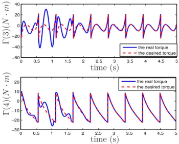
1.13 The torques of the swing leg for the control law based on tracking parametrized reference trajectory, where Γ(3) notes the torque of hip and Γ(4) notes the torque of knee. . . 36
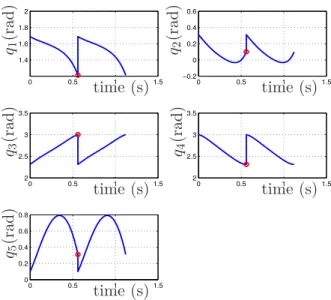
1.14 The difference of the real values and desired values of qu and ˙qu at the end of each step for the control law based on choice of controlled outputs with M1 = [0, 0, 0, 0]T. . . 37
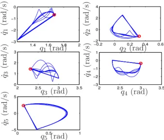
1.15 Phase-plane plots for qi, i = 1, . . . , 5 for the control law based on choice of controlled outputs with M1 = [0, 0, 0, 0]T. The straight lines correspond to the impact phase, where the state of the robot changes instantaneously. The initial state is represented by a (red) star. . . 37
1.16 The difference of the real values and desired values of qu and ˙qu at the end of each step for the event-based feedback control law. . . 39
1.17 Phase-plane plots for qi, i = 1, . . . , 5 for the event-based feedback control law. The straight lines correspond to the impact phase, where the state of the robot changes instantaneously. The initial state is represented by a
(red) star. . . 39
1.18 The torques of the swing leg for the event-based feedback control law, where Γ(3) notes the torque of hip and Γ(4) notes the torque of knee. . . 40
1.19 max |λ1,2| versus M1(j), j = 1, 2, 3, 4, when the other three components of M1 are zero. . . 41
1.20 The difference of the real values and desired values of qu and ˙qu at the end of each step for the control law based on choice of controlled outputs with M1 = [0, 0, −2.06, 0]T. . . 42
1.21 Phase-plane plots for qi, i = 1, . . . , 5 for the control law based on choice of controlled outputs with M1 = [0, 0, −2.06, 0]T. The straight lines correspond to the impact phase, where the state of the robot changes instantaneously. The initial state is represented by a (red) star. . . 42
1.22 The torques of the swing leg for the control law based on choice of controlled outputs with M1 = [0, 0, −2.06, 0]T, where Γ(3) notes the torque of torso and Γ(4) notes the torque of knee. . . 43
1.23 The height of the swing foot at the end of the step Zsw(Td) with respect to the effective eigenvalues of the Poincaré map, max |λ1,2|. . . 45
1.24 The stable domain of M1(2) and M1(3) for two groups of solution, which is described with contour line max |λ1,2|= 1 . . . 45
1.25 The difference of the real values and desired values of qu and ˙qu at the end of each step for the control law based on choice of controlled outputs with M1 = [1.91, −4, −3, −1.41]. . . . 46
1.26 The torques of the swing leg for the control law based on choice of controlled outputs with M1 = [1.91, −4, −3, −1.41], where Γ(3) notes the torque of hip and Γ(4) notes the torque of knee. . . 47
2.1 Photo of HYDROID . . . 51
2.2 Biped Model . . . 52
2.3 The support foot . . . 53
2.4 The definition of θ. . . . 55
2.5 Block diagram of the control system. . . 56
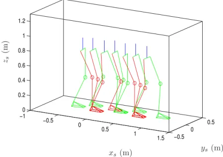
2.6 Stick-diagram for one step of the periodic walking gait in sagittal plane . . 64
2.7 max |λ1,2,3| versus M1(j, 1), j = 6, 7, when the other 9 components of M1 are zero. . . 65
2.8 Block diagram of the simulator. . . 66
2.9 The walking motion of first three steps with the proposed control law. . . . 67
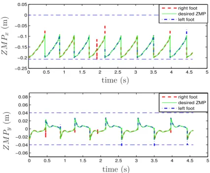
2.10 Position of ZMP with the proposed control law using the rigid ground model: the position of ZMP moves periodically and is always within the limits. . . 68
2.11 The tracking errors of q2with the proposed control law using the rigid ground model. . . 68
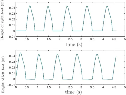
2.12 Height of feet with the proposed control law using the rigid ground model. 69
2.13 Phase-plane plots for qi, i = 1, 2, 3, 4 with the proposed control law using the rigid ground model. The initial state is represented by a (red) star. . . 69
2.14 Ground reaction force (GRF) of the soft ground model. . . 70
2.15 Position of ZMP in the feet sole with the proposed control law using the soft ground model: the position of ZMP moves periodically and returns to the limits fastly after impact. . . 71
2.16 Height of feet with the proposed control law using the soft ground model. . 71
2.17 Phase-plane plots for qi, i = 1, 2, 3, 4 with the proposed control law using the soft ground model. The initial state is represented by a (red) star. . . . 72
2.18 The tracking errors of q2 with the proposed control law using the soft ground
model. . . 72
2.19 Position of ZMP in the foot sole for the control law without the regulation of ZMPy: the position of ZMP moves periodically and is always within the limits but ZMPy does not track ZMPyd. . . 75 2.20 Phase-plane plots for qi, i= 1, 2, 3, 4 for the control law without the
regula-tion of ZMPy. The initial state is represented by a (red) star. . . 76 2.21 Height of feet for the control law without the regulation of ZMPy . . . 76 2.22 Position of ZMP in the foot sole for the control law without the regulation
of ZMPx: the position of ZMP moves periodically but ZMPx is out of the limit during a short time.. . . 79
2.23 Phase-plane plots for qi, i= 1, 2, 3, 4 for the control law without the regula-tion of ZMPx. The initial state is represented by a (red) star. . . 80 2.24 Height of feet for the control law without the regulation of ZMPx. . . 80 2.25 Position of ZMP in the foot sole for the control law without the regulation
of ZMP. . . 82
2.26 Phase-plane plots for qi, i= 1, 2, 3, 4 for the control law without the regula-tion of ZMP. The initial state is represented by a (red) star. . . 82
2.27 Height of feet for the control law without the regulation of ZMP. . . 83
2.28 Position of ZMP in the foot sole for the control law without the regulation of ZMP: the position of ZMPx is out of the limits when the larger initial errors are introduced. . . 83
2.29 Phase-plane plots for qi, i= 1, 2, 3, 4 for the control law without the regula-tion of ZMP when the larger initial errors are introduced. The initial state is represented by a (red) star. . . 84
2.30 Height of feet for the control law without the regulation of ZMP when the larger initial errors are introduced. . . 84
2.31 The tracking errors of q2 for the classical control law. . . 85
2.32 Height of feet with the classical control law, for the right foot a zoom is done along the vertical axis to show the unexpected rotation of the stance foot.. 86
2.33 COP in the feet sole for the classical control law. . . 86
3.1 Description of walking direction . . . 90
3.2 The positions of the feet at impacts with initial error of states, where the red points denote the midpoint of two feet. The robot departs from the direction of xs axis. . . 91 3.3 The modification of the reference path ud. . . . . 93 3.4 Scheme of the steering control law. . . 96
3.5 The positions of the feet at impacts under event-based feedback control, where the red points denote the midpoint of two feet. The robot walks along the direction of xs axis . . . 96 3.6 The direction angle of left foot ql, right foot qr and the walking direction
angle q0, where the straight lines in figures of ql and qr denote the single support phases. q0 converges to 180◦. . . 97
3.7 The positions of the feet at impacts under event-based feedback control, where the red points denote the midpoint of two feet. The robot walks along the direction of −xs axis . . . 98 3.8 The layout of the robot and the targets. . . 99
3.9 The positions of the feet at impacts for passing through the door, where the red points denote the midpoint of two feet. The walking path converges to the desired one yd= −0.5. . . . . 99 3.10 The direction angle of left foot ql, right foot qr, and the walking direction
angle q0, where the straight lines in figures of ql and qr denote the single support phases. q0is regulated to obtain yd= −0.5 at first, then it converges
to 0◦ so the robot walks along the x
s axis as shown in Fig. 3.9. . . 100 3.11 The positions of the feet at impacts for reaching two destinations at [6, 1]
and [6, −1] respectively. . . . 101
3.12 The relative distance of the robot and the destination at [6, 1]. . . . 101
4.1 HYDROID: biped robot with arms. . . 105
4.2 In case (a), the stance foot contacts the ground completely, the center of pressure of the forces on the foot, P, remains strictly within the interior of the footprint. In this case, the foot will not rotate, q1 = 0 and thus
the system is fully actuated. In case (b), the center of pressure has moved to the toe, that allows the foot to rotate, q1 6= 0, thus the system is now
under-actuated. . . 106
4.3 Human walking gait through one cycle, beginning and ending at heel strike. Percentages showing contact events are given at their approximate location in the cycle. Adapted from [Rose and Gamble, 1994]. . . 107
4.4 Walking gait of the studied robot with foot rotation phase. Adapted from [Tlalolini, 2008]. . . 108
4.5 The definition of θ during fully support phase (a) and foot rotation phase (b). Note that the definition of joint angle for the ankle and knee, i.e., q3
and q5, are different from that of the robot’s model shown in Fig. 2.4. This
is because the definition of coordinate systems for the two joints are changed in the new robot model. . . 110
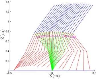
4.6 Stick-diagram for one step of the periodic walking gait in 3D space and sagittal plane. . . 115
4.7 max |λ1,2,3| versus M1(j, 1), j = 2, 16, when the other 22 components of M1
are zero. . . 116
4.8 Height of feet for the walking without foot rotation phase. . . 117
4.9 Position of ZMP in the foot sole for the walking without foot rotation phase: the position of ZMP moves periodically and is always within the limits. . . 117
4.10 Phase-plane plots for qi, i = 2, 3, 4, 5 for the walking without foot rotation phase. The initial state is represented by a (red) star. . . 118
4.11 The corresponding torques of qi, i = 2, 3, 4, 5 for the walking without foot rotation phase. . . 118
4.12 The walking motion of the robot without foot rotation phase during first three steps. . . 119
4.13 Stick-diagram for one walking step with foot rotation phase in 3D space. . 120
4.14 Stick-diagram for one walking step with foot rotation phase in sagittal plane.120
4.15 Foot rotation angle q1 and height of feet for the walking including foot
rotation phase. . . 121
4.16 max |λ1,2,3| versus M1(4, 1), when the other 22 components of M1 are zero. 122
4.17 Block diagram of the simulator for the walking with foot rotation phase. . 123
4.18 Height of feet for the walking including foot rotation phase. . . 124
4.19 Position of ZMP in the foot sole for the walking including foot rotation phase: the position of ZMP moves periodically. ZMPy is always within the limits and ZMPx is zero during under-actuated phase. . . 124 4.20 Phase-plane plots for qi, i= 2, 3, 4, 5 for the walking including foot rotation
phase. The initial state is represented by a (red) star. . . 125
4.21 The corresponding torques of qi, i= 2, 3, 4, 5 for the walking including foot rotation phase. . . 125
4.22 The tracking errors of q2 and q3 for the walking including foot rotation phase.126
4.23 The tracking errors of q14 and q15 for the walking including foot rotation
phase. . . 126
4.24 Rotation angle of the stance foot in the sagittal plane and its desired values. Note that in the first step it is q1 and in the next step is written as q16, and
so forth. . . 127
4.25 The walking motion of the robot with foot rotation phase during first three steps.. . . 127
4.26 Height of feet for the proposed control law considering initials errors and −20% modeling errors. . . 129
4.27 The tracking errors of q2 and q3 for the proposed control law considering
initials errors and −20% modeling errors. . . 129
4.28 Position of ZMP for the proposed control law considering initials errors and −20% modeling errors. ZMPy is always within the limits and ZMPx is zero during under-actuated phase. . . 130
4.29 Phase-plane plots for qi, i= 2, 3, 4, 5 for the proposed control law considering initials errors and −20% modeling errors. The initial state is represented by a (red) star. . . 131
4.30 The corresponding torques of qi, i = 2, 3, 4, 5 for the proposed control law considering initials errors and −20% modeling errors. . . 131
4.31 Position of ZMP for the proposed control law considering initials errors and +10% modeling errors. ZMPx almost reaches the edge of the heel during the fully support phase. . . 132
4.32 The tracking errors of q2 and q3 for the proposed control law considering
initials errors and +10% modeling errors. . . 132
4.33 Position of CoP in the foot sole for the walking with foot rotation phase under the classical control law: it moves out of the foot sole after walking two steps. . . 134
4.34 Height of feet for the walking with foot rotation phase under the classical control law. . . 134
4.35 The walking motion of the robot with foot rotation phase under the classical control law. . . 135
4.36 Phase-plane plots for qi, i= 2, 3, 4, 5 for the walking with foot rotation phase under the classical control law. The initial state is represented by a (red) star.135
B.1 The walking direction angle of the left foot before the impact of the first step with different δq0. The red point denotes the moment at Poincaré section
when δq0 is introduced in the feedback event-based control law. . . 160
B.2 The walking direction angle of the right foot before the impact of the second step with different δq0. Here the straight line denotes the right leg is
sup-ported by the ground in the first leg. The red point denotes the moment at Poincaré section where δq0 is introduced in the feedback event-based control
Research on biped humanoid robots is currently one of the most attractive topics in the field of robotics. Many biped walking robots have been manufactured since 1970s, such as
WL-12 [Yamaguchi et al., 1993], H5 [Nagasaka et al., 1999], ASIMO [Sakagami et al., 2002],
HRP-2 [Kaneko et al., 2004], QRIO [Ishida, 2004], JOHNNIE [Buschmann et al., 2007],
Lola [Buschmann et al., 2009]. Among them ASIMO of HONDA and HRP of AIST are
well known biped humanoid robots. Although more and more human-like biped robot plat-forms have been developed, the realization of stable walking of bipeds remains challenging. Compared to human walking, the walking of bipedal robots looks awkward and has less energetic efficiency. The foot rotation phase, where the stance heel lifts from the ground and the stance foot rotates about the toe, allows robot to reduce significantly the cost criterion for fast motions [Huang et al., 2001], [Tlalolini et al., 2009]. Work in [Kuo, 2002] shows that plantarflexion of the ankle, which initiates heel rise and toe roll, is the most efficient method to reduce energy loss at the subsequent impact of the swing leg. This motion is also necessary for the aesthetics of mechanical walking. Thus, it is extremely important and interesting to study the walking control of a humanoid robot with rotation of the feet, and that is also the ultimate goal of this thesis. However, the foot rotation phase is an under-actuated phase and the stability analysis is necessary during the design of the control law. In order to study the control of under-actuated biped robots and the principle of stability analysis using Poincaré method, our work starts with the research on RABBIT which is an under-actuated planar biped robot with point feet (4 actuated joints and 5 DOF). Based on this research, the walking control of a 3D biped robot with flat-feet but without arms (14 actuated joints) and the control of a 3D biped robot with arms (26 actuated joints) are studied. In the first two robot models, the walking phase only consists of single support phase and impact or instantaneous double support phase. In order to obtain a more human-like walking, the foot rotation phase is considered in the third robot model. As a preliminary study of our robot, the control laws proposed in this thesis use the principle of our earlier research. Specifically, the reference trajectory of the joint angles and ZMP have been off-line computed using the optimization techniques to
minimize the consumed torques [Chevallereau and Aoustin., 2001], [Tlalolini et al., 2011].
Our objective is to propose new control laws to satisfy the constraint of contact and to study the stability of walking, i.e., the convergence of periodical walking. The thesis is organized as follows.
In Chapter 1, the stable walking control of an under-actuated planar biped robot is
studied. The biped model consists of five links, connected together to form two legs
with knees and a torso (Fig. 1.3). It has point feet without actuation between the feet
and ground, so the ZMP heuristics is not applicable, and thus under actuation must be explicitly addressed in the walking controller design.
There exist various studies about the walking control of the under-actuated mechanical systems [Fantoni and Lozano, 2002], [Anderle and Celikovsky, 2009], [Grizzle et al., 2005],
[Zikmund and Moog, 2006], [Chemori and Loria, 2004]. Most controllers of these systems
are based on tracking reference motions. In the existing research of the biped, there are two groups of method which depend on the differences of reference trajectory. The first one is based on reference trajectory as a function of time and the latter one is time invariant. In the second method, for example, the method of virtual constraints, a state quantity of the biped which is strictly monotonic (i.e., strictly increasing or decreasing) along a typical walking gait, is used to replace time in parameterizing a periodic motion of the biped. When the reference walking motion is parametrized with respect to a scalar valued function of the state of the robot instead of time, the controller is time invariant, which helps analytical tractability. In addition, when such a control has converged, the configuration of the planar robot at the impact is the desired configuration. Moreover, it has been observed that for the same robot and for a same known cyclic motion, a control law based on a reference trajectory as a function of the state of the robot, produces a stable walking. Whereas a control law based on reference motion as a function of time produces
an unstable walking [Chevallereau, 1999]. For the above reasons, many walking controllers
are designed successfully based on this virtual constraints method for the planar bipeds in the previous work [Grizzle et al., 2001], [Chevallereau et al., 2003], [Plestan et al., 2003],
[Westervelt et al., 2003]. In [Shih et al., 2007] and [Chevallereau et al., 2009], this control
methodology has been extended to a 3D walking robot with 2 degree of under-actuation. However, the reference motion which is parametrized as a function of the state of the robot instead of time is not usual in robotics, while the definition of reference motion described as a function of time is more traditional. In addition, it is difficult to find the strictly monotonic state for some robots, for example, quadruped with a curvet gait, or biped with frontal motion [Kuo, 1999], [Fukuda et al., 2006].
Based on these observations, it is challenging and significantly important to propose a tool to analyze the stability of a control based on tracking reference motion as a function of time and to propose solution to obtain stable walking. This is exactly the purpose
of Chapter 1. The Poincaré method is used to numerically analyze the stability of limit
cycles for hybrid zero dynamics (HZD) of the robot. It has been proved that the closed-loop system is stable if and only if the eigenvalues of the linearized Poincaré map (ELPM)
have magnitude strictly less than one [Morris and Grizzle, 2009], [Westervelt et al., 2007,
Chap. 4]. Therefore, the control problem can be viewed as the problem of modifying the ELPM. Two control strategies are explored for the studied robot. The first strategy is
using event-based feedback control to modify ELPM. [Grizzle, 2003] shows that the
event-based feedback control could be used for the hybrid system with impulse effects such as the walking system of the biped robot. Here it is extended to a 2D biped robot with time-varying reference trajectory. It shows that this method is still usable, a vector of
parameters that is updated at each impact is introduced to modify the walking stride to stride.
The main contribution of Chapter 1 is the proposition of the second control law. In
contrast to the first control strategy, our second method does not need supplementary feedback controller. It is based on the choice of controlled outputs. When the controlled outputs are selected to be the actuated coordinates, most periodic walking gaits for this
robot are unstable. In [Wang et al., 2009] the effect of controlled outputs selection on the
walking stability was studied. It shows that the stable walking can be obtained by some pertinent choices of controlled outputs. These pertinent choices are not obvious. Is there a method to help with many judicious choices of controlled outputs to improve the stability? By studying some walking characteristics of many stable cases, we found that the height of swing foot is nearly zero for all the stable walking at the desired moment of impact for one
step. Consequently, that is viewed as a necessary condition proposed in Chapter1. Based
on this condition, the choice of controlled outputs is constrained, and then two stable do-mains for the controlled outputs selection are given. Finally, we compared the control
prop-erty of our second control law with the method of virtual constraints [Grizzle et al., 2001],
[Chevallereau et al., 2003], [Plestan et al., 2003], [Westervelt et al., 2003]. It shows that
when the controlled outputs are chosen pertinently, the velocity of the joints with our method converge faster than that with the method of virtual constraints.
As a following work, the principles of the control law and the method of stability
analysis in Chapter1are extended to the biped robot with feet. In Chapter2, some stable
walking control methods for a 3D bipedal robot with 14 joint actuators are proposed. As
shown in Fig. 2.2, the 3D robot is comprised of a torso and two identical legs that are
independently actuated and terminated with flat-feet.
The walking of biped robot with feet can be composed of different phases such as single support (SS) with flat foot, SS with foot rotation around the metatarsal axis and double support etc. During every walking phase, there is a corresponding dynamic model and condition of contact with the ground. Thus an appropriate control law has to be implemented for each phase. Generally, the sequence of type of contact with the ground is imposed but it is obtained only if the conditions of ground reaction force, friction cone and zero moment point (ZMP) are satisfied. The ZMP is firstly introduced by Vukobratovic
[Vukobratovic et al., 1990]. It is defined as a point about which the horizontal ground
reaction moment of the ground reaction force is zero. When this point is inside the support polygon, the robot will not rotate about the edges of the foot so the foot remains flat on the
ground. In this case, the ZMP is identical to the CoP (center of pressure) [Goswami, 1999].
In the earlier studies, many biped robots adopt a control strategy where the desired trajectories of joint angles are firstly designed based on the ZMP condition and then the
feedback control is executed for the designed ones [Vukobratovic et al., 1990]. However,
the contact condition cannot be satisfied in presence of perturbation. Therefore, most of the recent walking control strategies use ZMP and they are generally divided into two approaches.
First method is the periodical replaying of trajectories for the joint motions recorded in
little on-line modification. [Huang et al., 2000] and [Kim et al., 2006] proposed their real-time modification systems consisting of body posture control, actual ZMP control and landing time control based on sensor’s informations. These researches explicitly divide the problem into subproblems of planning and control.
The second method generates a joint-motion in real time, feeding back the present state of the system to be in accordance with the pre-provided goal of the motion, where
planning and control are managed in a unified way [Takeuchi, 2001], [Sugihara et al., 2002],
[Ferreira et al., 2006], [Coros et al., 2010], [Mitobe et al., 2000], [Kajita et al., 2001]. Two
of the more famous users of these methods are Honda Robot Asimo [K.Hirai et al., 1998]
and Kawada’s humanoid HRP-2 [S.Kajita et al., 2003], [S.Kajita et al., 2006]. Especially,
the control of ZMP proposed in [S.Kajita et al., 2003] was applied for the robot NAO in
the work of [Gouaillier, 2009].
In the above researches the robot is usually modeled as an inverse pendulum. The
inverse pendulum approximation is studied in [Miura and Shimoyama, 1984] for the
con-trol of the Biper-3 robot. In this approach, the whole mass of the robot is concentrated in one point, and the system dynamics are approximated using a simple inverted pen-dulum whose base represents the support foot during the single support phase. Kajita et al. [Kajita and Tani, 1991], [Kajita and Tani, 1995], [Kajita et al., 2001] extended the inverse pendulum approach and tested its validity on various robots. Errors between the computed motion of the inverted pendulum and the real motion of the robot must be compensated by feedback control. One solution is to use the actuated ankle joint and apply a small correcting torque. However, the single mass inverted pendulum is a non-minimum phase system, which imposes problems for controlling of the ZMP. Therefore
[Napoleon et al., 2002] proposed an extension toward a two mass inverted pendulum to
overcome this deficiency. [Sugihara and Nakamura, 2002] proposed a method to
manipu-late the CoG using the whole body motion, and to control the evolution of the inverted pendulum through ZMP manipulation.
The method that we developed belongs to a class of method that divides the problem into definition of reference motion and control. The control strategy can be viewed as an on-line modification of reference motion. In opposite to the methods based on inverted pendulum, a complete dynamic model is used. Our control law consists of ZMP controller, swing ankle rotation controller and partial joint angles controller. In the ZMP controller, the 2 positions of the calculated ZMP in the horizontal plane are regulated to follow the desired evolution of the ZMP. Since two torques will be used to insure that the ZMP evolution is correct, this means that not all the joints can be controlled directly. Because all of our work is done with a hypothesis that the ground is flat and the reference trajectory was planned to satisfy the condition of that the robot touches the ground with flat-foot, therefore, if the motion of all the joints can’t track the desired trajectory, the swing foot will not touch the ground with flat-foot. As a result, the support foot in the next step will not be flat, thus the control law will not be valid. The swing ankle rotation controller is used to solve this problem, in which the pitch and roll angle of the swing foot are controlled to follow their desired values. As in the case of under-actuated robot studied
As a consequence, the choice of controlled outputs of the partial joint angles controller depends on the stability analysis of the walking gait under closed-loop control.
In short, the ZMP controller and swing ankle controller are used to ensure the stability condition of supported foot and transferred foot respectively. The partial joint angles controller is used to track the reference trajectory and satisfy the stable condition of the overall control law. This control strategy is original for the biped robot with foot walking in 3D. As said in the beginning, almost all the existing on-line walking controllers are applied to compensate for the ZMP error. However, the general weakness of the previous methods is that they require considerable experimental hand tuning and these methods are poorly documented. Compared to these studies, our control law has the following advantages. The proposed method can be viewed as an on-line modification of the reference trajectory in order to insure the satisfaction of the constraint of contact. The main point is that the effect of this on-line modification on the stability of walking is studied based on rigorous stability analysis, not by testing on the robot which requires considerable experimental hand tuning.
In Chapter 3, the control of the walking direction without the modification of the
original reference trajectory is studied for the same biped robot studied in Chapter2. The
robot is expected to be able to move all over the working place when it works in human environment. Thus we need the precise steering control not merely the simple straight walking. Therefore, the objective of this chapter is to adjust the net yaw rotation of the robot over a step in order to steer the robot to walk along paths with mild curvature.
The walking direction control has been proposed by using the sophisticated trajectory
planning of CoG (center of gravity) and swing foot motion [Kajita et al., 2002], rhythmic
oscillators [S.Aoi et al., 2004], slip motion between sole and floor [Miura et al., 2008], or the
torsional deflection at the supporting foot [Oda and Ito, 2010]. Since the walking control
system proposed in Chapter 2 is based on tracking the off-line calculated joint motion, an
interesting feature of our walking direction control is that one is able to control the robot’s motion along various paths with limited curvature using only a single predefined periodic motion.
This work is extended from the previous studies for a 3D under-actuated biped robot
[Shih et al., 2010] and [Chevallereau et al., 2010]. The principle of our steering control
is to append an event-based feedback controller to distribute set point commands to all the actuated joints in order to achieve a desired amount of turning, as opposed to the
continuous corrections used in [Gregg and Spong, 2010]. Different from the other studies,
with our method the stability during steering is maintained.
Finally, in Chapter 4, the walking control law proposed in Chapter 2 is extended to a
humanoid robot with two arms. In addition, the walking phase describing the foot rotation around the metatarsal axis at the end of single support phase is included in the walking.
For walking gaits that include foot rotation, various ad-hoc control solutions have been
proposed in the previous literatures. For example, in [Takahashi and Kawamura, 2001]
the robot is controlled to track desired trajectories during foot rotation phase. The toe is modeled as a free joint because the input torque can not be applied to it. This kind of model produces a non-holonomic constraints system, of which the degree of freedom
degenerates. [Yi, 2000] proposed a walking control law for a biped robot with a compliant ankle mechanism. A pseudo static walking gait with dynamic gait modification method is presented by adjusting the position of a hip joint. The controller has two feedbacks, inner feedback for motor control and outer feedback for reference trajectory control. Be-sides of these, many researches considered the foot rotation phase in the jumping control
[Hyon et al., 2006], [Goswami and Vadakkepat, 2009] or the running control of the robots
[Kajita et al., 2007]. However, none of them can guarantee the stability in the presence of
the under-actuation that occurs during heel roll or toe roll. The approach developed in
[Choi and Grizzle, 2005] [Westervelt et al., 2007, Chap. 10] considers also a walking gait
with foot rotation and the walking stability during this phase is analyzed. The work in
[Chenglong et al., 2006] further elaborates on the Poincaré stability analysis of walking
gaits that include foot-rotation; in particular, the issue of the state dimension varying from one phase to another is emphasized. It shows that the feedback design methodology presented for robots with point feet can be extended to obtain a provably asymptotically stabilizing control law that integrates the fully actuated and under-actuated phases of walking.
Our work is extended from [Chevallereau et al., 2008], in which a control strategy for
simultaneously regulating the position of the ZMP and the joints of the robot was proposed for a biped robot in 2D. In addition, the proposed controller is based on a path-following control strategy, i.e., the reference trajectory is not defined as a function of time. This method with parametrized reference trajectory can deal with the under-actuation problem
during foot rotation phase. Therefore, since in Chapter2the proposed control law with this
kind of reference trajectory has been used successfully for the walking control of robot with flat-feet, the same control system can be used directly in the new robot with foot rotation phase. In order to consider all the effects of stance foot rotation on the dynamic models of robot, the foot rotation angle is viewed as an actuated joint angle to be considered in the joint configuration vector and used to calculate the forces and torques. As a result, a nominal torque at the toe of stance foot is calculated by using the dynamic model. In fact, during foot rotation phase, because the position of ZMP along x axis is zero so this torque is zero. Therefore, the proposed control law can be used in both of fully-actuated phase and foot rotation phase. Moreover, the stability during the foot rotation phase can also be taken into account, that is exactly what is missing in previous studies for walking gaits with foot rotation.
Walking control of an under-actuated
planar biped robot
1.1
Introduction
The primary objective of this chapter is to present three walking control laws that can achieve an asymptotically stable, periodic walking gait for an under-actuated planar biped robot.
The studied biped robot is RABBIT [Chevallereau et al., 2003] and it evolves only in
the sagittal plane. It consists of five links connected to form two legs with knees and a
torso (see Fig. 1.1) and it has point feet without actuation between the feet and ground.
First, the dynamic model of the robot during different walking phases are obtained by using the method of Lagrange. Next, a classical control strategy for under-actuated biped robots is presented at first. It is called virtual constraints method, in which a state quan-tity of the biped that is strictly monotonic along a typical walking gait, is used to
re-place time in parameterizing a periodic motion of the biped [Chevallereau et al., 2003],
[Plestan et al., 2003], [Westervelt et al., 2003], [Chevallereau et al., 2009]. With this
pa-rameterized reference trajectory, the controller is time invariant. When such a control has converged, the configuration of the planar robot at the impact is the desired configuration. Moreover, it has been observed that for the same robot and for a same given cyclic motion, a control law based on a parameterized reference trajectory produces a stable walking, whereas a control law based on reference trajectory as a function of time produces an
unstable walking [Chevallereau, 1999]. However, the parameterized reference trajectory is
not usual in robotics, while the definition of that as a function of time is more traditional. In addition, it is difficult to find the strictly monotonic state for some robots, for example,
robot-semiquad [Aoustin et al., 2005], quadruped with a curvet gait, or biped with frontal
motion [Kuo, 1999], [Fukuda et al., 2006].
Based on these observations, it is challenging and significantly important to propose a tool to analyze the stability of a control based on tracking reference trajectory as a function of time and to propose a solution to obtain stable walking. Therefore, the other
two walking control laws are proposed to track the reference trajectory expressed as a function of time. The second control law is obtained using event-based feedback control to
improve the walking stability, that is, the convergence of periodical walking. [Grizzle, 2003]
shows that it could be used for the hybrid system with impulse effects such as the walking system of the biped robot. With this control law, a vector of parameters that are updated just after each impact is introduced to modify the walking stride to stride. In this chapter it is extended to 2D biped robot with time-variant reference trajectory. It shows that this method is still usable.
In contrast with the second control strategy, the third method does not need supple-mental feedback controller. It is based on the choice of controlled outputs. For a robot has m actuators and point feet without actuation, the posture of the robot in the sagittal plane depends on m + 1 joint configuration variables but only m controlled outputs can be chosen. For simplicity, the m controlled variables are defined as a linear combination of m + 1 joint configuration variables. The most important question addressed in this control law is how this linear combination can be chosen in order to ensure walking sta-bility. The stability analysis is done with the method of Poincaré section, which is the classical technique for determining the existence and stability properties of periodic orbits
[Morris and Grizzle, 2009], [Westervelt et al., 2007, Chap. 4]. By introducing zero
dynam-ics, the stability of the walking gait under closed-loop control is evaluated in a reduced di-mensional space [Chevallereau et al., 2009], [Plestan et al., 2003], [Westervelt et al., 2003]. The numerical analysis shows that the stable walking can be obtained by using some per-tinent choices of controlled outputs. However, these perper-tinent choices are not obvious. Therefore, some walking characteristics of many stable cases are analyzed and a method to help with the selection of controlled outputs is proposed. Finally, three control methods are compared with each other.
This chapter is organized as follows. At first the studied robot is introduced in
Sec-tion 1.2 and its dynamic models during different walking phases are presented in Section
1.3. Next, a previous control law based on tracking parametrized reference trajectory is
introduced in Section 1.4. As a following work, other two control laws based on tracking
time-variant reference trajectory are proposed in Section1.5. At last, Section 1.6 gives the
simulation results under these three control laws and the conclusions are given in Section
1.7.
1.2
Description of the studied robot
1.2.1
Biped model
The studied robot is modeled based on RABBIT shown in Fig. 1.1. RABBIT was
designed and built between 1997-2001 by several French research laboratories such as IR-CCyN, LMS Poitiers, LSIIT, LAG, LVR Bourges, LRP, INRIA Rhone-Alpes and INRIA Sophia-Antipolis. A group of researchers constituted by IRCCyN, LGIPM Metz, LMS, GAL, LVR, LIRMM, LRP and LSS worked about this prototype in the project of ROBEA
"Walking and Running Control of a Biped Robot" between 2001 and 2004.
Figure 1.1: Photo of RABBIT
RABBIT was conceived to be the simplest mechanical structure that is still represen-tative of human walking. It is composed of a torso and two identical legs with point feet. The knees and the hips are actuated and they are one degree of freedom (DOF) rota-tional joints. Since RABBIT does not have foot, the ZMP heuristic is not applicable, and thus under-actuation problem must be explicitly addressed in the feedback control design, leading to the development of new feedback stabilization methods.
The studied biped robot is modeled in the sagittal xz plane. According to the mechan-ical structure of RABBIT, the model has a torso and two symmetric legs connected at a common point called the hip, and both leg ends are terminated in points. Obviously, there are 5 rigid links connected 4 ideal revolute joints at the knees and hips. Each revolute joint is independently actuated and the point of contact between the stance leg and ground is
under-actuated. Its geometric is shown in Fig. 1.2. The values of geometrical parameters
and other parameters are given in Table 1.1 and Table1.2, where:
• mi is the mass of the ith link with i = 1, . . . , 5, and i = 1, 3 denote the shins, i = 2, 4
denote the thighs and i = 5 denotes the torso. • Li is the length of the ith link.
• Si is the vector of the center-of-mass coordinates of the ith link.
• Ii is the moment of inertia of the ith link with respect to the y-axis .
• IA is the moment of inertia of each actuator with respect to the y-axis .
The posture of the biped is described by the vector q = [q1, . . . , q5]T (see Fig. 1.3). Since there is no actuation between the stance leg and ground, the unactuated variable is defined as qu = q1, then the vector of actuated variables is written as qa = [q2, . . . , q5]T.
Figure 1.2: Geometrical parameters of RABBIT
1.2.2
Walking gait
The gait is composed of single support phases and double support phases. The single
support phase or swing phase is defined to be the phase of locomotion where only one leg is
in contact with the ground. Conversely, double support is the phase where both feet are on the ground. It is supposed to be instantaneous and the associated impact can be modeled
as a rigid contact [Hurmuzlu and Marghitu, 1994]. At impact, the swing leg neither slips
nor rebounds, while the former stance leg releases without interaction with the ground. After that, both two legs exchange the role and the next single support phase will begin. The alternating phases of single support and double support (or impact) are defined as the
walking of robot, see Fig. 1.4.
Body shin(i = 1, 3) thigh (i = 2, 4) torso (i = 5)
mi (kg) 3.2 6.8 17.053
Li (m) 0.4 0.4 0.625
Si (m) 0.127 0.163 0.143
Ii (kg · m2) 0.1 0.25 1.869
Table 1.1: Geometrical parameters and dynamic parameters of the biped robot
Maximum torque Γmax (N · m) 150
Moment of inertia IA (kg · m2) 0.83
z
x
q1 q2 q3 q4 q5Figure 1.3: The studied biped
1.3
Dynamic model during different walking phases
1.3.1
Lagrange formulation
The dynamic model of a robot with several degrees of freedom can be obtained with the method of Lagrange, which consists of first computing the kinetic energy and potential energy of each link, and then summing terms to compute the total kinetic energy K,
and the total potential energy Ep. For the biped robot described by a set of generalized
coordinates q = [q1, . . . , qn]T, the Lagrangian is denoted by:
L(q, ˙q) = K(q, ˙q) − Ep(q) (1.1)
where ˙q = [ ˙q1, . . . , ˙qn]T is the vector of velocity, K is the total kinetic energy and Ep is the
total potential energy. The Lagrange equations are commonly written in the form:
d dt ∂L ∂˙q − ∂L ∂q = Qex (1.2)
where Qex represents the sum of the external forces and torques (moments) acting on the
robot. According to (1.1), (1.2) can be rewritten as:
d dt ∂K ∂˙q − ∂K ∂q + ∂Ep ∂q = Qex (1.3)
The kinetic energy of the system is a quadratic function in the joint velocities such that:
K = 1
2˙q
Figure 1.4: Walking phases
where D is a n×n symmetric and positive definite inertia matrix of the robot. Its elements
are function of the joint positions. Since the potential energy Ep is a function of the joint
positions , (1.3) and (1.4) lead to:
D¨q + C(q, ˙q) ˙q + G(q) = Qex (1.5)
where
• Dn×n is inertia matrix.
• Cn×n is Coriolis matrix.
• Gn×1 is gravity vector.
The matrices D, C and G can be calculated as [Dombre and Khalil, 1999]:
G = ∂Ep ∂q A = ∂∂2˙qK2 Cij = n X k=1 ci,jk˙qk with: ci,jk = 12[ ∂Dij ∂qk + ∂Dik ∂qj − ∂Djk ∂qi ]. (1.6)
For the studied robot, the computation of the sum of the external forces and torques Qex
is presented for two cases:
Force acting at the foot: Supposing that a force Fex = [Fx, Fz] is acting on the foot
at the point Xpi = [Xpix, Xpiz]T, we have:
Qexi = (
∂Xpi
∂q )
T
Torques acting at a revolute connection of two links: Supposing that a torque
τ is applied at a revolute joint connected two links and let θrel
j be the associated relative
angle, we have: Qexj = ( ∂θrel j ∂q ) Tτ. (1.8)
1.3.2
Swing phase model
As shown in Fig. 1.3, the swing phase model is created in the generalized coordinates
q = [q1, . . . , qn]T, where the unactuated variable is defined as qu = q1 and the vector of actuated variables is written as qa = [q2, . . . , q5]T. Since the robot’s legs are identical, in the stance phase, it will be assumed without loss of generality that leg-1 (left leg) is in contact with the ground. Moreover, the Cartesian position of the stance leg end will be identified with the origin of the xz-axes of the inertial frame.
Using the Lagrange formulation presented in Subsection 1.3.1, the dynamic model can
be written as:
D(qa)¨q + H(q, ˙q) = BΓ (1.9)
where H5×1 = C(qa, ˙q) + G(q) and D depends only on qa because the kinetic energy is
invariant under rotations of the body. B is obtained according to (1.8) and the definition
of q in Fig. 1.3, there is:
B = " 01×4 I4 # . (1.10)
Here and in the following contents, In denotes the identity matrix of dimension n × n.
1.3.3
Impact model
An impact occurs when the swing leg contacts the ground. The impact is modeled as a contact between two rigid bodies. Our objective is to obtain an expression for the generalized velocity just after the impact of the swing leg with the walking surface in terms of the generalized velocity and position just before the impact. The model from
[Hurmuzlu and Chang, 1992] is used here. The one difference is noted in the list of
hy-potheses [Westervelt et al., 2007]:
• HI1) an impact results from the contact of the swing leg end with the ground;
• HI2) the impact is instantaneous;
• HI3) the impact results in no rebound and no slipping of the swing leg;
• HI4) at the moment of impact, the stance leg lifts from the ground without
interac-tion;
• HI6) the actuators cannot generate impulses and hence can be ignored during impact;
• HI7) the impulsive forces may result in an instantaneous change in the robot’s
ve-locities, but there is no instantaneous change in the configuration.
The development of impact model involves the reaction forces at the leg ends, and thus
required (N + 2)- DoF, i.e., 7 -DoF model of the robot, see Fig. 1.2. Thus the Cartesian
position and velocity of the center of gravity are appended to the generalized configuration variables q. The extended generalized configuration variables in the double support phase are denoted by: qe= [q, xg, zg]T. Using qe in the method of Lagrange results in:
De(qa)¨qe+ He(qe, ˙qe) = BeΓ + Qexf, (1.11)
where Γ = [Γ1,Γ2,Γ3,Γ4]T is the vector of input torques and Qexf represents the vector
of external forces action on the robot due to the contact between the leg ends and the
ground. According to the definition of qe, De can be described by:
De = " D(qa) 05×2 02×5 mtoI2 # . (1.12)
where mto is the total mass of the robot.
Here we use "−" to denote the moment just before impact and "+∗" to denote the moment just after impact but before the exchange of legs. From Hypothesis HI7, during the impact, the biped’s configuration variables do not change, that means:
qe+∗ = q
−
e (1.13)
However, the generalized velocities undergo a jump during the impact. This jump is linear
with respect to the joint velocity before the impact ˙q− [Westervelt et al., 2007]. Under
Hypothesis HI1 − HI7, "integrating" (1.11) over the "duration" of the impact and using (1.7) gives: " D(q− a) 05×2 02×5 mtoI2 # ( ˙q+∗ e − ˙q − e) = ( ∂Xpi(q−) ∂qe )T Fex (1.14)
where the subscript i denotes that leg-i is the swing leg before impact, the Cartesian
position of the end of leg-i Xpi can be expressed in terms of the Cartesian position of the
center of gravity and the robot’s angular coordinates as:
Xpi= " xg zg # − fi(q) (1.15)
where fi = [fix, fiz] is determined from the robot’s parameters (links lengths, masses,
positions of the center of mass). Next, (1.15) leads to:
∂Xpi ∂qe =h −∂fi ∂q I2 i 2×7. (1.16)
Substituting (1.16) into (1.14) yields: " D(q− a) 05×2 02×5 mtoI2 # ( ˙q+∗ e − ˙q − e ) = − ∂fi(q−) ∂q T I2 Fex (1.17)
The vector Fex of the ground reaction impulse can be expressed using the last two lines of
the matrix equation in (1.17):
Fex = mto( " ˙x+∗ g ˙z+∗ g # − " ˙x− g ˙z− g # ) (1.18)
Since two legs touch the ground during the impact, according to (1.15), there is:
" ˙x+∗ g ˙z+∗ g # = ∂fi(q−) ∂q ˙q +∗, " ˙x− g ˙z− g # = ∂fj(q−) ∂q ˙q − , (1.19)
where the subscript j denotes the stance leg before impact.
Substituting (1.19) and (1.18) into (1.17), the robot’s angular velocity vector after
impact is given by a linear expression with respect to the velocity before impact: ˙q+∗ = I(q− ) ˙q− (1.20) with I(q− ) = (D + mto ∂fi ∂q T∂f i ∂q) −1 (D + mto ∂fi ∂q T∂f j ∂q). (1.21)
Since we are assuming a symmetric walking gait, we can avoid using two single support models, one for each leg playing the role of the stance leg, by relabeling the coordinates at impact. The coordinates must be relabeled because the roles of the legs must be swapped: the former swing leg is now in contact with the ground and is poised to take on the role of the stance leg. Combining (1.13) with (1.20) and defining "+" denotes the moment after impact and after the exchange of legs, the joint configuration and velocity becomes:
(
q+ = Eq−
˙q+ = EI(q−) ˙q− , (1.22)
where E is a (5 × 5) matrix which describes the transformation of two legs, and it is:
E = 1 1 1 −1 −1 0 0 0 0 1 0 0 0 1 0 0 0 1 0 0 0 1 0 0 0 . (1.23)
1.3.4
Hybrid model of walking
An overall model of walking is obtained by combining the swing phase model and the im-pact model to form a system with impulse effects. It can be expressed as a nonlinear hybrid system containing two state manifolds (called "charts" in [Guckenheimer and Johnson, 1995]).
Define the state variables of robot as x = [q, ˙q]T, so the state before impact is noted as
x− = [q−
, ˙q−]T, and the state after impact and after the exchange of legs is noted as
x+ = [q+, ˙q+]T. With the application of (1.9) and (1.22), a complete walking motion of
the biped robot is written as Σ : ( ˙x = f(x) + g(x) uτ x−∈ S/ x+ = ∆(x−), x− ∈ S , (1.24) with f(x) = " ˙q −D−1(q a)H(q, ˙q) # , g(x) = " 05×4 D−1(q a) B # , uτ = Γ and x+ = ∆(x− ) = " E EI(q−) # x− .
where S is a hyper surface at which solutions of the differential equation undergo a discrete transition that is modeled as an instantaneous reinitialization of the differential equation.
S is called the impact surface and S = {(q, ˙q)|Zsw(q) = 0, Xsw(q) > 0}, where Zsw,
Xsw describe the position coordinates of swing foot along z and x axis respectively. Here
Xsw(q) > 0, because the swing leg is supposed to be placed strictly ahead of the stance
leg.
The equation (1.24) means that a trajectory of the hybrid model is specified by the
swing phase model until an impact occurs when the state of robot attains the set S. At this point, the impact of the swing leg with the walking surface results in a change in the velocity components of the state vector. The impulse model of the impact compresses the impact event into an instantaneous moment in time, resulting in a discontinuity in the velocities. The ultimate result of the impact model is a new initial condition from which the swing phase model evolves until the next impact. In order for the state not to be obliged to take on two values at the impact moment, the impact event is described in terms of the values of the state just before impact and after impact. These values are
represented by the left and right limits, x− and x+, respectively. Solutions are taken to be
right continuous and must have finite left and right limits at impact.
1.4
A control law for tracking parametrized reference
trajectory
This section will propose a previously studied control strategy of the under-actuated biped robot, i.e. the method of virtual constraints, which has been proved very suc-cessful in designing feedback controllers for stable walking in planar under-actuated bipeds
[Chevallereau et al., 2003], [Plestan et al., 2003], [Westervelt et al., 2003], [Westervelt et al., 2002]. Since not all the joints can be controlled for the studied under-actuated robot, the stability
of the periodic walking gait under the closed-loop control law must be analyzed. In order to simplify the stability analysis, the definition of zero dynamics will be introduced.
1.4.1
The reference trajectory
Using optimization techniques developed in [Djoudi et al., 2005], an optimal cyclic
mo-tion qd(t) has been defined for the robot Rabbit described in Section1.2. The most
impor-tant point of the method of virtual constraints is that qd(t) is parametrized by a quantity
that only depends on the states of robot and is strictly monotonic like time t during the walking phase. By using this method, the closed-loop system does not depend on the time
t thus only the kinematic evolution of the robot’s state is regulated but not its temporal
evolution. That means the control law is defined to follow a joint path but not a joint motion.
In a forward human walking motion, the x-coordinate of the hip is monotonically in-creasing. Hence, if the virtual stance leg is defined by the line that connects the stance foot to the stance hip, the angle of this leg in the sagittal plane is monotonic and it can
replace the time t to parametrize qd. As shown in Fig.1.5, because the shin and the thigh
have the same length, this angle can be computed by:
θ = q1+ q2/2. (1.25) z x q1 q2 θ Figure 1.5: Description of θ
Next, because the obtained reference trajectory is a set of discrete points, in order to approximate the desired cyclic motion for each of the five configuration coordinates, a
one-dimensional Bezier polynomial [Bezier, 1972] with order J = 5 is chosen to describe
the reference trajectory. It is:
hd(s) = J X k=0 αk J! k!(J − k)!s k(1 − s)J −k , (1.26)
where the coefficient αk is determined to minimize the distance between the optimal
tra-jectory and reference tratra-jectory at the discrete points, and
s= θ − θi
θf − θi
(1.27)
is the normalized parameter varying on the cyclic motion from 0 to 1. θi and θf are the
values of θ at the beginning and end of a step respectively. Using (1.27), the parametrized
reference trajectory in (1.26) can also be written as hd(θ), and it is such that: qd(t) = hd(θ) ˙qd(t) = ∂hd(θ) ∂θ ˙θ ¨qd(t) = ∂2hd(θ) ∂θ2 ˙θ 2+∂hd(θ) ∂θ ¨θ (1.28) Here and in the following contents the superscript "d" means the desired value. In
[Djoudi et al., 2005], the evolution of the joints variables qd was assumed to be polynomial
function of a scalar path parameter such as s in (1.27). The coefficients of the polynomial
functions were chosen to optimize a torque criterion and to insure a cyclic motion for the biped. Finally, some discrete points of the reference trajectory qd(t), ˙qd(t), ¨qd(t) were
calculated thus they are supposed to be known in this thesis. From these results, in (1.28)
hd(θ), ∂hd(θ)
∂θ and
∂2hd(θ)
∂θ2 can be deduced by (1.26) and its differential coefficients, so they
are also supposed to be known in the following contents.
1.4.2
Calculation of the input torques
Since only the actuated joints are controlled and their joint configurations are q2, q3, q4, q5, the controlled variables are written as:
u= Mq (1.29)
with
M =h 04×1 I4
i
. (1.30)
The unactuated joint angle q1 is not controlled at all. The 4 outputs that must be zeroed
by the control law are:
y= u − ud(θ) (1.31)
where ud(θ) is the desired value of the controlled vector u. The PD controller is used to
obtain u = ud, the expected acceleration ¨u is defined as:
¨u = ¨ud−Kd
ε ( ˙u − ˙u
d) −Kp
ε2 (u − u
d), (1.32)
where Kp >0, Kd>0, and ε > 0. According to the definition of u, here ¨ud, ˙ud and ud can
be calculated by M and the obtained reference trajectory in (1.28).
ud(θ) = Mhd(θ) ˙ud(θ) = M∂hd(θ) ∂θ ˙θ ¨ud(θ) = M(∂2hd(θ) ∂θ2 ˙θ2+ ∂hd(θ) ∂θ ¨θ) (1.33)
Next is how to compute the input torques based on (1.32). Because ud and its
differ-ential coefficients are functions of θ, using (1.25), (1.29), q can be described by:
q= T−1 q " θ u # . (1.34) with Tq = 1 0.5 0 0 0 0 1 0 0 0 0 0 1 0 0 0 0 0 1 0 0 0 0 0 1 . (1.35)
Thus, substituting (1.34) into the dynamic model during the swing phase (1.9) yields:
DT " ¨θ
¨u
#
+ H(q, ˙q) = BΓ, (1.36)
where DT = DTq−1. Defining DT and H as:
DT = " DT11(1×1) DT12(1×4) DT21(4×1) DT22(4×4) # , H = " H1(1×1) H2(4×1) # , (1.37)
(1.36) can be rewritten as:
(
DT11¨θ+ DT12¨u + H1 = 0
DT21¨θ+ DT22¨u + H2 = Γ
(1.38) Substituting (1.32) and (1.33) into the first line of (1.38), ¨θ is solved at first:
¨θ = −H1− DT12Ua DT11+ DT12M∂h d(θ) ∂θ (1.39) with Ua = M ∂2hd(θ) ∂θ2 ˙θ 2− Kd ε ( ˙u − ˙u d) − Kp ε2 (u − u d). (1.40)
Then the input torques can be calculated by substituting ¨θ in the second line of (1.38):
Γ = DT22Ua+ (DT21+ DT22M
∂hd(θ)
∂θ )¨θ + H2. (1.41)
1.4.3
Stability analysis
Many robot motions are naturally periodic. The periodic behavior is also called limit cycle. Limit cycles can be stable (attracting), unstable (repelling) or non-stable (saddle)
[Hiskens, 2001]. The classical technique for determining the existence and stability
![Figure 1.15: Phase-plane plots for q i , i = 1, . . . , 5 for the control law based on choice of controlled outputs with M 1 = [0, 0, 0, 0] T](https://thumb-eu.123doks.com/thumbv2/123doknet/7801032.260848/50.918.274.614.470.771/figure-phase-plane-plots-control-choice-controlled-outputs.webp)
![Figure 1.21: Phase-plane plots for q i , i = 1, . . . , 5 for the control law based on choice of controlled outputs with M 1 = [0, 0, −2.06, 0] T](https://thumb-eu.123doks.com/thumbv2/123doknet/7801032.260848/55.918.275.614.581.881/figure-phase-plane-plots-control-choice-controlled-outputs.webp)