De-anonymization attack on geolocated data

HAL Id: hal-01242268

https://hal.archives-ouvertes.fr/hal-01242268

Submitted on 11 Dec 2015

HAL is a multi-disciplinary open access

archive for the deposit and dissemination of

sci-entific research documents, whether they are

pub-lished or not. The documents may come from

teaching and research institutions in France or

abroad, or from public or private research centers.

L’archive ouverte pluridisciplinaire HAL, est

destinée au dépôt et à la diffusion de documents

scientifiques de niveau recherche, publiés ou non,

émanant des établissements d’enseignement et de

recherche français ou étrangers, des laboratoires

publics ou privés.

De-anonymization attack on geolocated data

Sébastien Gambs, Marc-Olivier Killijian, Miguel Nuñez del Prado Cortez

To cite this version:

Sébastien Gambs, Marc-Olivier Killijian, Miguel Nuñez del Prado Cortez. De-anonymization attack

on geolocated data. Journal of Computer and System Sciences, Elsevier, 2014, 80 (8), pp.1597-1614.

�10.1016/j.jcss.2014.04.024�. �hal-01242268�

De-anonymization attack on geolocated data

a_{Universit´e de Rennes 1 - INRIA/ IRISA, Campus Universitaire de Beaulieu 35042 Rennes, France} b_{LAAS - CNRS, 7 avenue du Colonel Roche, BP 54200, F-31031 Toulouse, France}

c_{Universit´e de Toulouse, INSA, LAAS, F-31400 Toulouse, France}

Abstract

With the advent of GPS-equipped devices, a massive amount of location data is being collected, raising the issue of the privacy risks incurred by the individuals whose movements are recorded. In this work, we focus on a specific inference attack called the de-anonymization attack, by which an adversary tries to infer the identity of a particular individual behind a set of mobility traces. More specifically, we propose an implementation of this attack based on a mobility model called Mobility Markov Chain (MMC). A MMC is built out from the mobility traces observed during the training phase and is used to perform the attack during the testing phase. We design several distance metrics quantifying the closeness between two MMCs and combine these distances to build de-anonymizers that can re-identify users in an anonymized geolocated dataset. Experiments conducted on real datasets demonstrate that the attack is both accurate and resilient to sanitization mechanisms such as downsampling.

Keywords: Privacy, geolocation, inference attack, de-anonymization.

1. Introduction

With the recent advent of ubiquitous devices and smartphones equipped with positioning capacities such as GPS (Global Positioning System), a massive amount of mobility traces is collected and gathered in the form of geolocated datasets by cellphone companies, providers of location-based services, and developers of smartphone applications. Some of these geolocated datasets are available in public repositories and can be used for research or for industrial purposes (e.g., to optimize the placement of cellular towers, to conduct market and sociological studies or to analyze the flow of traffic inside a city). These datasets are composed of the mobility traces of hundreds or thousands of individuals [1, 2, 3, 4], thus raising the issue of the privacy risks incurred by these individuals. For instance, from the movements of an individual it is possible to infer his points of interests (such as his home and place of work) [5, 6, 7, 8], to predict his past, current and future locations [9, 10], or even to infer his social network [11].

In this work, we focus on a particular form of inference attack called the de-anonymization attack, by which an adversary tries to infer the identity of a particular individual behind a set of mobility traces. More precisely, we suppose that the adversary has been able to observe the movements of some individuals during a non-negligible amount of time (e.g., several days or weeks) in the past during the training phase. Later, the adversary accesses a different geolocated dataset containing the mobility traces of some of the individuals observed during the training phase, plus possibly some unknown persons. Then, the objective of the adversary is to de-anonymize this dataset (called the testing dataset) by linking it to the corresponding individuals contained in the training dataset. Note that simply replacing the real names of individuals by pseudonyms before releasing a dataset is usually not sufficient to preserve the anonymity of their identities because the mobility traces themselves contain information that can be uniquely linked back to an individual. In addition, while a dataset can be sanitized before being released by adding spatial and temporal noise, the risk of re-identification through de-anonymization attack nevertheless still exists. Thus, in order to be able to assess the importance of this risk, it is important to develop a method to quantify it.

∗

Corresponding author

Email addresses: [email protected] (S´ebastien Gambs), [email protected] (Marc-Olivier Killijian), [email protected] (Miguel N´u˜nez del Prado Cortez)

In this paper, we propose a novel method to de-anonymize location data based on a mobility model called Mobility Markov Chain (MMC) [7]. A MMC is a probabilistic automaton, in which each state corresponds to one (or possibly several) Point Of Interest (POI), characterizing the mobility of an individual and an edge indicates a probabilistic transition between two states (i.e., POIs). Each state can have an semantic label attached to it such as “home”, “work”, “leisure”, “sport”, . . . A MMC is built out of the mobility traces observed during the training phase and is used to perform the de-anonymization attack during the testing phase. More precisely, the mobility of each individual both from the training and testing sets is represented in the form of a MMC. Afterwards, a distance is computed between possible pairs of MMCs from the training and testing sets in order to identify the closest individuals in terms of mobility. In short, the gist of this method is that the mobility of an individual can act as a signature, thus playing the role of a quasi-identifier [12]. Thus, if the adversary knows a target user Alice and a signature of her mobility (e.g., he has learnt her MMC out of the training set), he can try to identify her by finding a matching signature in the testing set.

The outline of the paper is the following. First, in Section 2, we review some related work on de-anonymization attacks and mobility models before briefly introducing in Section 3 the background on Mobility Markov Chains necessary to understand our work. Afterwards in Section 4, we present the distance metrics between MMCs that we designed in order to quantify the closeness between two mobility behaviors, while in Section 5 we describe how to build predictors (which we call de-anonymizers) based on these distances to efficiently and accurately de-anonymize location data. Finally, we evaluate experimentally the efficiency of the proposed attack on real geolocated datasets in Section 6 before concluding in Section 7.

2. Related work

An inference attack corresponds to a process by which an adversary that has access to some data related to indi-viduals (and potentially some auxiliary information) tries to deduce new personal information that was not explicitly present in the original data. For instance, a famous inference attack was conducted by Narayanan and Shmatikov on the “Netflix dataset” [13]. This dataset is a sparse high dimensional data containing ratings on movies of more than 500 000 subscribers from Netflix that was supposed to have been anonymized before its release for the Netflix compe-tition1_{. However, Narayanan and Shmatikov have performed a de-anonymization attack that was able to successfully}

re-identify more than 80% of the Netflix subscribers by using the Internet Movie Database2_{(IMDB), a public database}

of movie ratings, as auxiliary knowledge.

Inference attacks have also been developed specifically for the geolocated context. For instance, Mulder et al. [6] have proposed two methods for profiling users in a GSM network that can also be used to perform a de-anonymization attack. The first method is based on constructing a Markov model of the mobility behavior of an individual while the second considered only the sequence of cell IDs visited. Once POIs have been extracted for each user, an agglom-erative hierarchical clustering algorithm is used to group users according to a similarity measure called the cosine similarity[14]. Their first method is relatively similar to ours with two major differences due to the fact that their dataset comes from a cellular network. Thus, it relies on the static GSM cells as the states of the Markov model, while we dynamically learn the POIs from the mobility traces of an individual. Therefore, in our setting two individuals do not necessarily have any POI in common, whereas with GSM cells, individuals living in the same area have a high probability of sharing some POIs (i.e., cells). As a consequence, the second main difference between their work and ours is that the transitions are only possible between neighboring GSM cells, as it is impossible to “jump” from one cell to another if they are not adjacent. Their attack was validated through experimentations using cell locations of 100 users from a MIT Media Lab dataset3_{[15] that includes information such as call logs, Bluetooth devices in proximity,}

cell tower IDs, application usage and phone status. During the experiments, the authors have observed that if the currently profiled user belongs to a cluster of other similar users, there is a high chance of making a mistake about the identity inferred among all the users of this cluster when performing the de-anonymization attack. The success rate of the re-identification attack varies from 37% to 39% using the Markov model, against 77% to 88% when the sequence of cells visited is used.

1_{http://www.netflixprize.com} 2_{http://www.imdb.com}

Zang and Bolot [8] have performed a study of the top n most frequently visited places by an individual in a GSM network and show how they can act as quasi-identifiers to re-identify anonymous users. Their study was performed on the Call Data Records (CDRs) from a nationwide US cellular provider collected over a month and contains approxi-mately 20 millions users. From this dataset, the authors have identified the top n most frequent places for each user at different levels of spatial (i.e., sector, cell, zip code, city, state and country) and time granularity (i.e., day and month). Their inference attack was able to successfully re-identify 35% of the population studied when the adversary has no auxiliary knowledge and even up to 50% when the adversary can use the knowledge of the social network of users as auxiliary information. The social network was constructed by creating a social relationship between two individuals that have called each other at least once in the past. In their analysis, the authors emphasize that the distance between home and work can be an indicator of the privacy level for an individual. In particular, the larger this distance, the higher the risk that this individual can be de-anonymized.

Ma et al. [16] proposed an inference attack to de-anonymize users in a geolocated dataset along with a metric to quantify the privacy loss of an individual. Two datasets were used in this study, one recording the movements of San Francisco YellowCabs [1] and the other related to the movements of Shanghai city public buses4. Two types of adversary models were considered: the passive one, collecting the whereabouts of individuals from a public source (possibly sanitized) and the active one that can deliberately participate or perturb the data collection in order to gain additional knowledge about the location of some specific individuals. To retrieve the identities of individuals, the authors imagine four different estimators that the adversary can use to measure the similarity between mobility traces (for instance between the original traces and the sanitized ones). Namely, the Maximum Likelihood Estimator relies on the Euclidean distance to compute the similarity between mobility traces. The Minimum Square Approach computes the negative sum of the square of the absolute value of the difference between the original traces and the sanitized ones. The Basic Approach assumes that the traces have been perturbed by uniform noise. Thus with this approach, a mobility trace will be considered to be similar to another trace if it is contained within a sphere of radius rcentered on the original trace. Finally, the Weighted Exponential Approach is similar to the Basic Approach, with the exception that no assumption is made on the type of noise generated. These methods approach a success rate of de-anonymization of 80% to 90% on the San Francisco YellowCabs dataset and between 60% and 70% on the Shanghai bus dataset, and this even when the data is sanitized through the addition of spatial noise. However, contrary to our work, these inference attacks were conducted on the whole dataset (there was no split between a training set and a testing set). In particular, the authors assume that both type of adversaries (i.e., passive and active ones) pick the information they need to build the mobility model from the same dataset on which the success of the de-anonymization attack is tested. This induces an overly strong bias in the re-identification results obtained with this approach.

The work of Freudiger, Shokri and Hubaux [17] also focuses on re-identifying users of geolocated datasets. These experiments have been conducted on two datasets. The first dataset5_{contains the GPS traces of 24 users from the city}

of Borlange recorded in a two-year period (1999-2001) while the second one is due to Nokia6_{and is composed of the}

GPS traces of 150 users from the city of Lausanne recorded over a year. In this work, the pair of POIs “home/work” is used as pseudo-identifiers to de-anonymize users. First, a variant of the k-means algorithm is used to extract POIs from the mobility traces. Then, the POI in which the individual considered stays the most often between 9PM to 9AM is identified as “home” while the POI in which the individual stays the most often between 9AM to 5PM is labelled as “work”. The training phase consists in applying this method on the raw data to extract the pairs “home/work” for all individuals, and then to conduct the same attack on sampled traces in order to assess how much the pair “home/work” can still be inferred even when the dataset released has been sanitized by applying sampling. The success of this method depends on how sampled traces have been generated. Indeed, the authors have proposed several sampling schemes whose bias towards selecting home/work locations or other POIs can be parametrized. The authors have shown that when 100 samples are observed, the de-anonymization rate is approximately 67% for the Borlange dataset and 70% for the Nokia one. Unfortunately, as most of the previous works presented, this study does not split the available data into a training and testing set during its evaluation but rather generates the samples that will constitute the testing set directly from the training one. This introduces a major bias in the evaluation of the techniques, which we further discuss in Section 6.4.

4_{To the best of our knowledge, this dataset is not publicly available contrary to the other one.} 5_{http://icapeople.epfl.ch/freudiger/borlange.zip}

The work of Xiao et al. [18] relies on the notion of Semantic Location Histories (SLH) to compute the similarity between users. In a nutshell, a SLH is simply the sequence of semantic locations frequently visited by an individual. Like several previous approaches, this work first uses a hierarchical clustering algorithm to extract POIs out of mobility traces. Then, using as external knowledge a database that can associate semantics to a location, each POI is linked with a semantic tag for each level of the hierarchy (e.g., “Italian restaurant” and then “restaurant” at an upper level). Finally, the SLH is computed by analyzing the sequence of POIs visited by a user and taking into account their semantic labels. The similarity measure designed by the authors is based on the notion of maximal travel match, which counts the number of similar semantic locations visited (not necessarily in the same order) by two different SLHs within a predefined time interval. This metric is computed for each layer of the cluster hierarchy before being summed over all possible layers, possibly by weighting the influence of a particular level (i.e., the deeper the level, the bigger the influence). Finally, the proposed approach was evaluated on the Geolife dataset [19]. Contrary to previous work, the success of the de-anonymization attack is quantified in terms of the normalized discounted cumulative gain, a metric originated from information retrieval [20]. In a nutshell, the objective of this metric is to rank all the possible candidates to de-anonymization with respect to how close their mobility is to the behavior of the user considered. In the experiments conducted, the success of the attack as measured by this metric was between 0.7 and 0.9. Basically the closer this value is to 1, the more effective the attack is. Note that, due to the different metric that was used, this method is not directly comparable to other previous works.

Shokri et al. [21] inferred the correspondence between pseudonymized traces of 40 randomly chosen users of the YellowCabs dataset [1], in which each position is a cell of 8×5 grid over the San Francisco Bay area, and user profiles represented in the form of hidden Markov model. Their attack computes a matching probability between pseudonymized traces and user profiles by using the classical forward-backward algorithm [22]. This matching prob-ability basically represents the likelihood that a particular set of traces correspond to a specific user. Once these probabilities are computed, a bipartite graph of traces and users is formed whose edges are weighted according to the associated matching probability between pairs of user/traces. This bipartite graph is then given as input to the Hungarian algorithm that assign a particular set of traces to each user. As the paper mainly focuses on solving the task of “individual tracking”, which corresponds to being able to predict at which location a user was located at a particular moment in time, their results are not directly comparable to our work. However, we believe that the framework they have developed is generic enough in terms of the attacks it encompasses that it could also model the de-anonymization attack.

The study of Srivatsa and Hicks [23] de-anonymizes users based on the contact graph, generated from mobility traces and information about their social network. The authors use three different datasets: the Saint Andrews dataset, which contains 18 241 contact traces from 27 different users issued from WiFi access points, the Smallblue dataset is formed by 240 665 contact traces of 125 users representing messages generated by instant messaging, and finally the Infocom 06 dataset that consists of 182 951 contact traces from 78 users extracted from Bluetooth devices used during the Infocom 2006 conference. In addition, the authors have used some auxiliary knowledge in the form of social networks extracted from Facebook for the Saint Andrews and Smallblue datasets and from DBLP for the Infocom 06 dataset. Their attack relies on the structural similarities between contact and social graph, which is measured in terms of standard graph similarity measures such as the graph edit distance (i.e., minimal number of edges to erase or add to have a perfect match), the maximum common subgraph (i.e., the number of vertices in the largest common subgraph) and the distribution of node degrees. The de-anonymization attack works in two steps. During the fist step, the n most important POIs are extracted from both contact and social graphs based on the node centrality metric [24]. The second step is the de-anonymization process itself that links the identities of users from the social graph with the corresponding users of the contact graph. The authors have used three different mapping techniques: distance vector (82% of de-anonymization rate), spanning trees (88% of de-anonymization rate) and subgraph matching (80% of de-anonymization rate).

Sharad and Danezis [25] have de-anonymized the communication graph datasets of the D4D challenge7_{. Their}

attack exploits the topology of the contact graph to break the anonymity by looking for subgraphs that are isomorphic and form the largest subgraphs. More precisely, the authors compute the 1-hop node neighborhood degree distribution for each node of the subgraphs generated from the graph. This distribution is used as a similarity metric to identify the

7

closest node with the same characteristics in the other graph. Afterwards, for matching the 2-hop nodes, the authors rely on two metrics: the neighbor match, which is the number of common 1-hop nodes they are associated to, and the signature match, which is a metric computed from the in and out degree distributions. To evaluate their methodology, Sharad and Danezis have used the EU mail communication dataset [26] and artificially generated a dataset with similar characteristics to the communication graphs of the D4D challenge obtaining between 56% to 96% of re-identification rate.

A recent study of De Montjoye and co-authors [27] has shown that if an individual has a unique pattern in the anonymized dataset then this is enough to characterize him even if a particular dataset does not contain personal information such as name, age and address. The objective of this study was precisely to measure the uniqueness of 1.5 millions users in an anonymized mobile phone dataset collected from April 2006 to June 2007. By taking 2 and 4 random locations to characterize the mobility patterns of individuals, the authors were able to identify respectively 50% and 95% of the users in the anonymized dataset. However, this study has some limitations as for instance it is not clear how the knowledge that is learnt can be used to later in the future de-anonymize an individual. More precisely, the study shows that during a particular period (e.g., a day or a week) if we consider the sequence of a constant number locations visited by an individual compared to the rest of the population, this sequence is likely to be unique. Nonetheless, this do not preclude the possibility that other individuals might visit the same sequence of locations during another period (e.g., the next day or the next week). Thus, it is not obvious how to build an efficient de-anonymizer from the results of this study. Moreover as for other previous works, there is no separation being made between the training and the testing sets in this study.

Name Location data Strategy Re-identification

rate

Location profiling GSM [6] Call data records Markov chain

Sequence of visited places

37%-39% 77%-88% Most frequented

POIs [8]

Call data records and

social network Top n visited locations 35%-50%

Similarity between

trajectories [16] GPS traces Similarity of trajectories 60%-90%

Pair home/work [17] GPS traces Pair home/work used

as quasi-identifiers 67%-70%

Semantic location

histories [18] GPS traces Semantic trajectories 70%-90% (NDCG)

Likelihood between

traces and users [21] GPS traces Hungarian algorithm Not applicable

Linking nodes [23] GPS traces and

social network

Structural similarities between

contact and social graphs 82%-88%

Structure of the graph [25] Communication graph Structural similarities

between graphs 56%-96%

Random locations [27] Call data records Use of random locations

as quasi-identifiers 50%-95%

Summary statistics [28] Connections to access points Similarity between spatial

distributions of users 43%-71%

Table 1: Summary of related work.

Finally, a recent work by Unnikrishnan and Naini [28] shows that revealing statistics about the movements of users (instead of directly their mobility traces) can also be used to de-anonymize efficiently geolocated datasets and thus may also be harmful to privacy. To perform the de-anonymization attack, the authors computed through the Hungarian algorithm the minimum weight matching [29] in a bipartite graph, composed of an anonymous and labeled graph, in which nodes represent users and the weights on edges correspond to the distance in term of entropy between the spatial and temporal distribution of nodes across different places. The dataset used is a two weeks logs obtained from the access points from the EPFL campus, using the first week for training and the second one for testing. Using

this technique, the authors obtained 70.5% of success for the de-anonymization.

In this section, we have reviewed the previous work on de-anonymization attacks in the geolocated context, which we summarize in Table 1. Note that the results from some of these studies cannot be directly compared due to the difference in nature of the datasets used, the way the success metrics are defined for an attack and also the fact that in most of these studies the data has not been split in proper training and testing sets. We discussed further this fundamental issue in Section 6.4. In the following sections, we will present our approach to de-anonymization. More precisely, we first introduce how to model the mobility of an individual in the form of a MMC, before describing how to measure the similarity between two MMCs using the distances we propose. Finally, we demonstrate experimentally how to use these distance metrics to perform a de-anonymization attack.

3. Mobility Markov Chain

A Mobility Markov Chain (MMC) [7] models the mobility behavior of an individual as a discrete stochastic process in which the probability of moving to a state (i.e, POI) depends only on the previously visited state and the probability distribution on the transitions between states. More precisely, a MMC is composed of:

• A set of states P= {p1, . . . pn}, in which each state is a frequent POI (ranked by decreasing order of importance),

with the exception of the last state pnthat corresponds to the set composed of the union of all infrequent POIs.

POIs are learned by running a clustering algorithm on the mobility traces of an individual. These states are associated to a location, and generally they also have an intrinsic semantic meaning. Therefore, semantic labels such as “home” or “work” can often be inferred and attached to them.

• Transitions, such as ti, j, represent the probability of moving from state pito state pj. A transition from one state

to itself is possible if the individual has a non-null probability from moving from one state to an occasional location before coming back to this state. For instance, an individual can leave home to go to the pharmacy and then come back to his home. In this example, it is likely that the pharmacy will not be extracted as a POI by the clustering algorithm, unless the individual visits this place on a regular basis and stays there for a significant amount of time.

Note that several mobility models based on Markov chains have been proposed in the past [7, 30], including the use of hidden Markov models for extracting the semantics of POIs [31]. In a nutshell, building a MMC is a two-steps process. During the first phase, a clustering algorithm is run to extract the POIs from the mobility traces. For instance in the work of Gambs et al. [7], a clustering algorithm called Density-Joinable Cluster (DJ-Cluster) was used (we rely on the same algorithm in this work), but of course other clustering algorithms are possible. In the second phase, the transitions between those POIs are computed and incorporated in the MMC.

DJ-Cluster takes as input a trail of mobility traces and four parameters: the minimal number of points MinPts needed to create a cluster, the maximum radius r of the circle within which the points of a cluster should be contained, the minimal number of days that the traces falling within a cluster should cover and d a threshold distance used to decide if two neighboring clusters should be merged. DJ Cluster works in three phases. During the first phase, which corresponds to a preprocessing step, all the mobility traces in which the individual is moving (i.e., whose speed is above a small predefined value) as well as subsequent static redundant traces are removed. As a result, only static traces are kept. The second phase consists in the clustering itself: all remaining traces are processed in order to extract clusters that have at least MinPts points within a radius r of the centre of the cluster. Finally, the last phase merges all clusters that have at least a trace in common or whose medoids are within d distance of each other. Once the POIs (i.e., the states of the Markov chain) are discovered, the probabilities of the transitions between states can be computed. To realize this, the trail of mobility traces is examined in chronological order and each mobility trace is tagged with a label that is either the number identifying a particular state of the MMC or the value “unknown”. Finally, when all the mobility traces have been labeled, the transitions between states are counted and normalized by the total number of transitions in order to obtain the probabilities of each transition. A MMC can either be represented as a transition matrix or as a graph in which nodes correspond to states and arrows represent the transitions between along with their associated probability. When the MMC is represented as a transition matrix of size n × n, the rows and columns correspond to states of the MMC while the value of each cell is the probability of the associated transition between the corresponding states.

4. Distances between mobility Markov chains

In this section, we propose four different distances quantifying the similarity between two mobility Markov chains. These distances are based on different characteristics of the MMCs and thus give different but complementary results. We will rely on these distances in the following sections to perform the de-anonymization attack.

4.1. Stationary distance

The intuition behind the stationary distance is that the distance between two MMCs can be evaluated as to the sum of the distances between the closest states of both MMCs. In order to compute the stationary distance, the states of the MMCs are paired in order to minimize this distance. As a result, it is possible that a state from the first MMC is paired with several states of the second MMC (this is especially true if the MMCs are of different size). Furthermore, the computation of the stationary distance heavily relies on the stationary vectors of the MMCs. In a nutshell, the stationary vector of a MMC is a column vector V, obtained by multiplying repeatedly a vector initialized uniformly Vinitby the MMC transition matrix M until convergence (i.e., until the distribution of values in this vector reaches the

stationary distribution of the MMC).

The stationary distance is directly computed from the stationary vectors of two MMCs (hence its name). More precisely, given two MMCs, M1and M2, the stationary vectors, respectively V1and V2, of each model are computed.

Afterwards, Algorithm 1 is run on these two stationary vectors. For each state in V1, the algorithm searches for

the closest state in V2 (lines 5 to 11, Algorithm 1) and then multiplies the distance between these two states by the

corresponding probability of the stationary vector of the state of V1currently considered (line 12, Algorithm 1).

Once the algorithm has taken into account all states from V1, the current value computed represents the distance

from M1 to M2 (distanceABin line 1, Algorithm 2). This distance is not symmetric as such and therefore in order

to symmetrize it, Algorithm 1 is called once again, but on V2and V1 in order to obtain the distance from M2 to M1

(distanceBAof line 2, Algorithm 2). The result is made symmetrical by computing the average of these two distances

(line 3, Algorithm 2).

Algorithm 1 Stationary distance(V1, V2)

1: distance= 0

2: for i= 1 to n1(the number of nodes in V1) do

3: MinDistance= 100000 kilometers

4: Let pibe the ithnode of V1

5: for j= 1 to n2(the number of nodes in V2) do

6: Let pjbe the jthnode of V2

7: CurrentDistance= Euclidean Distance(pi, pj)

8: if (CurrentDistance < MinDistance) then

9: MinDistance= CurrentDistance

10: end if

11: end for

12: distance= distance + ProbV1(pi) × MinDistance

13: end for

14: return distance

Algorithm 2 Symmetric stationary distance(V1, V2)

1: distanceAB= Stationary distance(V1, V2)

2: distanceBA= Stationary distance(V2, V1)

3: distance= (distanceAB+ distanceAB)/2

4.2. Proximity distance

The intuition behind the proximity distance is that two MMCs can be considered close if they share “important” states. For instance, if two individuals share both their home and place of work they should be considered as being highly similar. Moreover, the importance of a state is directly proportional to the frequency at which it is visited. Therefore, the first states ordered by decreasing order of importance are compared, then the second ones, then the third ones, and so on. The proximity score obtained for sharing the first states is considered twice as important as the score for sharing the second states, which is itself twice as important as the sharing of the third states, and so forth.

Given two MMC models M1and M2(ordered in a decreasing manner with respect to their stationary probabilities),

this distance is parametrized by a threshold∆ and a rank. The objective of the rank is to quantify the importance of matching two states at a specific level. In particular, the higher is the value of the rank, the bigger is the weight that will be given to these POIs. For instance for the first pair of POIs, we have set rank= 10.

Algorithm 3 starts by verifying for each pair of nodes between M1and M2if the Euclidean distance between them

is less than the threshold∆ (line 8, Algorithm 3). If this condition is met, the value of rank is added to the score value (line 9, Algorithm 3). Afterwards, rank is divided by two (lines 11-14, Algorithm 3). Once all the pair of nodes have been processed, the global distance is set to be the inverse of the global score if this score is non-null (lines 17-19, Algorithm 3). Otherwise, the distance outputted is set to a large value (e.g., 100 000 kilometers).

Algorithm 3 Proximity distance(V1, V2, ∆, rank)

1: Sort the states of V1by decreasing order of frequency

2: Sort the states of V2by decreasing order of frequency

3: score= 0

4: for i= 1 to min(n1, n2) do

5: Let pabe the ithnode of V1

6: Let pbbe the ithnode of V2

7: distance= Euclidean distance(pa, pb)

8: if (distance <∆) then

9: score= score + rank

10: end if 11: rank= rank/2 12: if (rank= 0) then 13: rank= 1 14: end if 15: end for 16: distance= 100000 17: if (score > 0) then 18: distance= 1/score 19: end if 20: return distance 4.3. Matching distance

The matching distance is similar to the stationary distance in the sense that this distance also corresponds to the sum of distances between the states of these two MMCs. However, the pairing of the states between the MMCs is done in a different way as each state from the first MMC is paired with one and only one state of the second MMC.

The matching distance is based on the Hungarian method [32], which is a polynomial-time combinatorial opti-mization algorithm for assignment problems. More precisely, the method works as follows. Given two MMCs, M1

and M2and their corresponding stationary vectors V1and V2, Algorithm 4 first verifies if the number of nodes in both

models is the same. If not, we assume without loss of generality that M2is the MMC with the fewer number of states.

Before continuing the computation of the distance, “dummy” states are added to M2. Each dummy state is a copy of

the centroid of the states of M2(line 4, Algorithm 4). Once this process is completed, the number of states in V1and

Algorithm 4 Matching distance(V1, V2)

1: Let D be the distance matrix D and Min the minimization matrix

2: Let n1be the number of nodes in V1

3: Let n2be the number of nodes in V2(we suppose that V2is the stationary vector with the fewest number of states

if the number of states between V1and V2is different)

4: Add fake states to V2if necessary to ensure that n2= n1

5: for i= 1 to n1do 6: for j= 1 to n2do 7: Di, j= Euclidean distance(pi, pj) 8: if (pior pjis fake) then 9: Mini, j= 100000 10: else 11: Mini, j= Di, j 12: end if 13: end for 14: end for 15: Index= HungarianAssignment(Min) 16: Dist= 0 17: for i= 0 to n1do

18: row= Indexi,0

19: col= Indexi,1

20: if (V2.node(col) is not fake) then

21: proba= (V1(row)+ V2(col))/2

22: Dist= Dist + Drow,col× proba

23: else

24: proba= (V1.stationaryVector(row) + 0)/2

25: Dist= Dist + NearestState(V1.node(row), V2.nodes)

26: end if

27: end for

Afterwards, the distance matrix (Di, j) and the minimization matrix (Mini, j) are computed. The distance matrix contains the Euclidean distance between each pair of nodes in M1and M2(lines 5-14, Algorithm 4), in which nodes

in M2form the rows of the matrix and nodes in M1correspond to the columns of Di, j. For instance, the distance Di, j

is the Euclidean distance between the node i in M2and the node j in M1. The minimization matrix is equivalent to the

distance matrix, except that each distance Mini, jin which node i is a dummy is assigned a large default value, such as

100 000 kilometers (line 9, Algorithm 4). In short, the objective of this large value is to guide the Hungarian method towards giving priority to real states instead of dummy ones.

The minimization matrix, which is squared, is passed as input to the Hungarian method. The Hungarian method then computes the optimal assignment between states from M1 and M2 that minimizes the global sum of distances

between pair of states and such that each state from V1is exactly matched with one state of V2(and vice-versa). This

optimal matching is returned as a matrix Index composed of two columns. Each column contains respectively the indexes of rows and columns of the optimal assignment for the minimization matrix Mini, j. Figure 1 illustrates graph-ically an optimal assignment between two MMCs (one for Alice and one for Bob). The matrix Index corresponding to Figure 1 is I= {{1, 1}, {2, 3}, {3, 2}, {4, 3}, {5, 4}}.

Alice MMC. Bob MMC.

Figure 1: Example of the optimal matching of two MMCs. The number in each node corresponds to the numbers of traces that falls inside this state.

For each pair of the matching obtained, the distance between these two (non-dummy) states is multiplied by the average of probabilities of stationary vectors V1 and V2. However, when one of the state in M2 is “dummy”, the

nearest real state in M2is identified, and the distance between these two states is then multiplied by the probability

corresponding to the “orphan” state in V1divided by two (lines 17–27, Algorithm 4). The distance returned is the sum

of the values computed for each pair of the matching (line 28, Algorithm 4). 4.4. Density-based distance

Similarly to the stationary and the matching distances, the density-based distance is simply the sum of the distances between pairs of MMCs states. However, the MMCs states are paired according to their rank once they are sorted using their corresponding probabilities in the stationary vector.

First, given two MMC models M1and M2, the nodes in both models are sorted by decreasing density (lines 1 and

2, Algorithm 5). Therefore, the first node will be the one with the highest stationary probability. Afterwards, the first node of M1is matched with the first node of M2and the same goes for the rest of the nodes. Finally, the sum of all

distances between matched nodes is computed (line 4 to 8, Algorithm 5) and the algorithm outputs the total distance. The stationary distance, the matching distance and the density-based distance are all numerical, in the sense that they are formed of the sum of the Euclidian distance between some pairing of states. In contrast, the proximity distance is different as it is based on the semantics behind the MMCs. Indeed, the first state in the model is inferred as being very representative of the mobility of an individual (e.g., home), the second as quite representative (e.g., the place of

Algorithm 5 Density − based distance(V1, V2)

1: Sort the states of V1by decreasing order of density

2: Sort the states of V2by decreasing order of density

3: distance= 0

4: for i= 1 to min(n1, n2) do

5: Let pabe the ithnode of V1

6: Let pbbe the ithnode of V2

7: distance= distance + Euclidean distance(pa, pb)

8: end for

9: return distance

work), and two individuals are considered as very similar if they share these two places. Table 2 summarizes the main characteristics of these distances. Thereafter, we will see how these distance can be used to build de-anonymizers and how their diversity can be exploited and combined to enhance the success of the de-anonymization attack.

Name Strategy Type Complexity

Stationary distance Stationary vector Numerical O(n)

Proximity distance Proximity of MMCs states Relative O(n)

Matching distance Hungarian algorithm Numerical O(n3₎

Density-based distance Weight of MMC states Numerical O(n)

Table 2: Summary of MMC distances. In this table, the (computational) complexity is measured with respect to n the number of individuals in the datasets that has to be de-anonymized (for simplicity the training and testing datasets are assumed to contained the same number of individuals).

5. De-anonymizers

In this section, we rely on the four distances proposed in the previous section to build statistical predictors in order to perform a de-anonymization attack. We call such a predictor, a de-anonymizer in reference to its main objective. A de-anonymizer takes as input the MMC representing the mobility of an individual and tries to identifies within a set of anonymous MMCs, the one that is the most similar (i.e, the closest in terms of distance). For example, a de-anonymizer may learn from the training set a MMC representing the mobility of Alice and later look for the presence of Alice in the testing set. A de-anonymizer can be based on one distance or a combination of them.

• The minimal distance anonymizer considers that in each row (i.e., a row refers to an individual to de-anonymize), the MMC with the minimal distance (i.e., the column) is the individual corresponding to the identity of the row. We have considered four instantiations of this de-anonymizer, one for each of the dis-tance previously described (i.e., stationary disdis-tance, proximity disdis-tance, matching disdis-tance and density-based distance).

• The maximal-gap de-anonymizer takes as input several distance matrices corresponding to different distance metrics. For each distance matrix, the minimal distance de-anonymizer outputs two predictions (instead of one) for each row, which corresponds to the first and second smallest values of the distances in this row. Afterwards, the gap (i.e, difference) between these two values are computed. The higher the gap, the more confident we can be in the prediction made by the de-anonymizer on this particular distance matrix. Therefore, the distance metric with the highest gap among all the ones considered will be the candidate considered for the de-anonymization. • The simple vote de-anonymizer receives as input a list of candidates, which corresponds to the identities of the n minimal values of a particular row in at least two different distance matrices. The candidate that receives the highest number of votes will be the one considered for the de-anonymization. For example, in Table 3, each column corresponds to different distance metrics while each row contains the proposed candidates at this position. In the first row, Bob gets two votes against one for Alice and therefore he is considered as the most likely candidate for de-anonymization.

Points m1 m2 m3

3 Bob Alice Bob

2 Charlie Bob Alice

1 Alice Charlie Charlie

Table 3: Illustration of the voting method, each colum corresponds to the output of a de-anonymizer based on a different distance metric.

• The weighted vote de-anonymizer, much like the simple vote one, takes as input a list of candidates coming from different distance matrices. However, the voting method weights each possible candidate depending on the rank he has obtained for the different distance metrics. For instance, if each distance metric proposes n candidates, the first one is given a weight n, while the second receives a weight of n − 1, and so on. For example, in Table 3, the first column contains the weights for each candidate. In this particular case, the outcome of the weighted voting method is that Bob gets 8 votes, Alice 6 and Charlie 4. Therefore, Bob is considered as the “winner” (i.e., most likely candidate) for the de-anonymization.

• The stat-prox de-anonymizer behaves exactly like the minimal stationary distance de-anonymizer, except when the stationary distance is above a given threshold and the proximity distance is below its maximum value (i.e., 100 000 kilometers). The intuition is that if the minimal stationary distance is very small, we should use it. Otherwise, we rely on the minimal proximity distance unless it gives no conclusive result, in which case we roll back to the minimal stationary distance.

6. Experiments Link MMCs with identities Sp lit d a ta se ts Adversary's auxiliary knowledge MMC mo d e ls G e o lo ca te d D B Si mi la ri ty ma tri x

Training set Testing set

T ra in in g se t Te st in g se t Identities D e -a n o n ymi za tio n Ground truth De-anonymization attack

An overview of the process of de-anonymization attack over geolocated datasets used in our experiments is il-lustrated in Figure 2. Considering a particular geolocated dataset, we first sort the mobility traces of each user in a chronological order. Then, for each user his trail of mobility traces is split into two disjoint trail of traces of same size, one for the training set and one for the testing set as explained in Section 6.1. The former is part of the auxiliary knowledge gathered by the adversary while the latter is the ground truth we use to assess the success of the attack. For each of this dataset, we learn a MMC for each trail of mobility traces. With respect to the MMCs learnt from the training set, the adversary knows the correspondence between these models and the corresponding identities of the users. Afterwards, the distances described in Section 4 are used to compute a distance matrix between the MMC models resulting from the training and testing sets. Subsequently, using this distance matrix as input to one of the de-anonymizer described in Section 5, the objective of the de-anonymization attack is to map back the users of the testing set to their true identities by linking their models in the testing set to the corresponding ones in the training set. Finally, the success rate of the attack is computed by measuring the ratio between the number of correct predictions over the total number of guesses. In order to estimate the robustness of the de-anonymization attack when the sampling conditions change, we have also performed some downsampling on the data. In a nutshell, a sampling mechanism summarizes several mobility traces into fewer traces. This is generally done by representing a set of subsequent traces that have occured within the same time window into a single trace (e.g., the average or median trace).

We evaluate the efficiency of the de-anonymization attack introduced in the previous section on five different datasets described in Section 6.1. Then, we describe the method used to fine-tune the parameters of the clustering algorithms in Section 6.2. Afterwards, we report the results of those experiments that were conducted by using the distances and anonymizers described in the previous sections. More precisely, we evaluate the accuracy of the de-anonymization attack relying on either a single predictor or a combination of them (Section 6.3). Finally, in Section 6.4, we compare our work with the performance reported in related works, highlighting in particular the bias in some of the experimental settings of these previous works.

6.1. Description of datasets

The datasets used in the experiments are described thereafter.

1. The Arum dataset [4] is composed of the GPS traces of 5 researchers sampled at a rate of 1 to 5 minutes in the city of Toulouse from October 2009 to January 2011.

2. The Geolife dataset [19] has been gathered by researchers from Microsoft Asia and consists of GPS traces collected from April 2007 to October 2011, mostly in the area of Shanghai city. This dataset contains the mobility traces of 178 users captured at a very high rate of 1 to 5 seconds.

3. The Nokia dataset [2] is the result of a data collection campaign performed the city of Lausanne for 200 users started in September 2009 and that lasted for more than two years. The rate at which the location has been sampled varies depending on the current battery level.

4. The San Francisco Cabs (SFC) dataset [1] contains GPS traces of approximately 500 taxi drivers collected over 30 days, between May and July 2008, in the San Francisco area.

5. The Borlange dataset [17] has been collected as a part of traffic congestion experiment over two years from 1999 to 2001. The public version of this dataset contains the GPS traces of 24 vehicles.

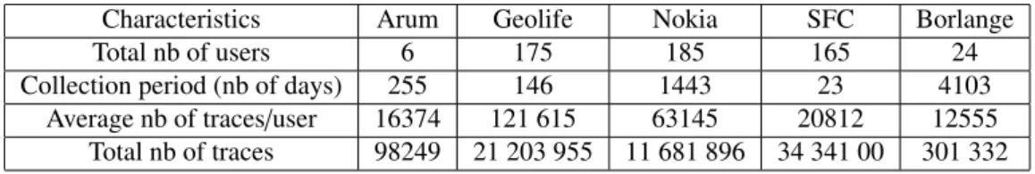
Table 4 summarizes the main characteristics of the datasets described above, namely the total number of users in the dataset, the collection period measured in the number of days as well as the average number of traces per user and the total number of traces in the dataset.

Characteristics Arum Geolife Nokia SFC Borlange

Total nb of users 6 175 185 165 24

Collection period (nb of days) 255 146 1443 23 4103

Average nb of traces/user 16374 121 615 63145 20812 12555

Total nb of traces 98249 21 203 955 11 681 896 34 341 00 301 332

Conducting an analysis of the distribution of the average number of traces per user, we have observed that there is a high variance with a large gap between the users with a small number of traces compares to the one with a high number of traces. For instance in Figure 3, we have shown the distribution of the users according to their number of traces for the Geolife and Nokia datasets. While these distributions are peaked around the category of users that have between 1000 and 10000 traces, the other categories of users also contains a significant number of users. With respect to the other datasets (Arum, SFC and Borlange), they are close to be uniformly distributed with the exception of the SFC dataset, which also displays a peak distribution.

0   20   40   60   80   100   120   [0  -­‐  10^2  >   [10^2  -­‐  10^3    >   [10^3  -­‐  10^4>   [10^4  -­‐  10^5>   [10^5  -­‐  10^6>   [10^6>   Num be r  of  use rs   Geolife   Nokia  

Figure 3: Distribution of the users according to their number of traces for the Geolife and Nokia datasets.

For each individual, we split his trail of mobility traces (chronologically ordered) into two disjoint parts of ap-proximately the same size. The first half of the original data forms the training set, and will be used as the adversary background knowledge, while the second half constitutes the testing set on which the de-anonymization attack is conducted. For instance, if the original trail of one individual is composed of n mobility traces {mt1, mt2, . . . , mtn}, it

will be split into a training set {mt1, mt2, . . . , mtn

2} and a testing set {mtn2+1, mtn2+2, . . . , mtn} (for illustration purpose we assume that n is an even number). Therefore, the objective of the adversary is to de-anonymize the individuals of the testing set by linking them to their corresponding counterparts in the training set. For simplicity reason, we assume thereafter that the training and the testing set are composed of the same n persons while in general this might not be the case (e.g., the testing set could only contain a small fraction of the users of the training set). Of course, dividing the training and test sets based on the number of traces may not guarantee that the length (i.e., number of days) of the period they covered is exactly the same.

In order to evaluate the impact of the size of the training set on the construction of a MMC, we have varied its size between 10% to 50% of the total number of traces, trying all slices by range of 10%. The value of 50% corresponds to the original “full” training dataset composed of the first half of the trail of traces. We choose to use the stationary distance (cf. Section 4.1) as a direct measure of the similarity between the MMC learnt on the reduced training set and the one learnt on the full training set. More precisely, a small stationary distance between the reduced training MMC and the full training MMC means that the two models are quite similar and thus that there was enough information contained in the considered training set to build a “representative MMC”. From Figure 4, we can observe that the more traces are used to build the training MMC, the smaller the stationary distance becomes between the reduced training MMC and the full training MMC. In particular, it seems that we need at least 30% of the total of the mobility traces to build a compact and representative MMC model.

In the following, we first focus on the Geolife dataset in order to analyze and understand the behavior of the de-anonymizers and distances.

40 50 60 70 80 90 0 10 20 30

Training (40%) Training (30%) Training (20%) Training (10%) Nokia GeoLife

Figure 4: Stationary distance between the “reduced” training set and the “full” training set for the Geolife and the Nokia datasets, when the size of the training set varies between 10% to 50% of the total number of traces.

6.2. Fine-tuning clustering algorithms and de-anonymizers

The states of a MMC are extracted by running a clustering algorithm on the mobility traces of an individual. Therefore, the MMC generated (and by extension the success of the de-anonymization attack) is highly dependent on the clustering algorithm used and the accuracy of this algorithm, which may itself vary depending on the values of its parameters. The first step of our analysis consists in determining the parameters that leads to the best accuracy for the DJ-clustering algorithm.

Depending on the chosen values for the parameters, not all users of the original Geolife dataset will lead to the generation of a well-formed MMC. For instance, when the parameters of the clustering algorithm are too “conserva-tive”, some users will not have enough mobility traces to identify frequent POIs, which results in their MMC being composed of only one state. On the contrary, choosing parameters that are too “relaxed” leads to the identification of a high number of POIs thus conducting to a MMC with too many states, which is detrimental to the success of the de-anonymization attack. Thus, the main objective of the tuning phase is to find the good set of parameters for the clustering algorithm that maximize the number of users in the training set whose MMCs does not consist in only one state while keeping the average number of POIs identified per user in an acceptable range.

First, we vary the three parameters of the clustering algorithm (MinPts, r and the minimal number of days) and count the number of MMC generated that have more than one state. We found that these parameters are themselves highly correlated with the duration of the collection period and the sampling rate used. Table 5 summarizes the values of the clustering parameters used in the following experiments obtained after this validation process.

Data set MinPts r(km) Minimal nb of days

Arum 40 0.05 30

Geolife 20 0.5 10

Nokia 10 0.05 10

SFC 20 0.05 10

Borlange 2 0.05 10

Table 5: Validated clustering parameters.

Once the parameters of the clustering algorithm have been tuned, we have assessed the efficiency of the simple and weighted voting de-anonymizers. In particular for the simple voting method, we first studied the influence of

the number of candidates proposed by the minimal distance de-anonymizer used on each distance metric (stationary, matching, proximity and density-based). Each instance of this de-anonymizer proposes the n candidates that have the smallest distances in a row sorted in increasing order. The simple vote de-anonymizer is applied to this list of candidates in order to output a single prediction. Figure 5 illustrates the success rate of this attack as a function of the number of candidates (more precisely as the percentage of true positives obtained over the total number of individuals) and the number of users that have well-formed MMCs (i.e., MMCs that have more than one state). This experiment was conducted on the Geolife dataset with the sampling rate varying in the range {10s, 30s, 60s, 120s}.

0%   5%   10%   15%   20%   25%   30%   35%   40%  

5s  (81  users)   10s  (77  users)   30s  (71  users)   60s  (67  users)   120s  (59  users)  

Su cc es s   ra te  (%)  

Sampling  rate  in  seconds  

1  candidate     2  candidates   3  candidates   4  candidates  

Figure 5: Success rate with the simple vote function.

0%   5%   10%   15%   20%   25%   30%   35%   40%  

5s  (81  users)   10s  (77  users)   30s  (71  users)   60s  (67  users)   120s  (59  users)  

Su cc es s   ra te  (%)  

Sampling  rate  in  seconds  

Linear   Exponen;al  

Figure 6: Success rate of the linear/exponential weighted votes.

From Figure 5, we can observe that the number of users considered that have a well-formed MMC decreases as the sampling rate increases, because a low sampling rate results in fewer mobility traces to build MMCs. We can also observe that the success rate of the attack decreases as the number of candidates increases, which is not surprising as a higher number of candidates renders the task of the de-anonymizer more complex that when they are few candidates. For instance, the success rate of the attack when 4 candidates are generated by each distance metric is never more than 15%. Therefore, we can conclude that for the simple vote method considering only one candidate per distance is sufficient.

However, in some situations it is helpful to consider more than one candidate per distance metric but their weight should be set to be different values, which is the main idea behind the weighted vote de-anonymizer. In our exper-iments, we have compared two different ways to weight candidates, one based on linear weights and the other on exponential ones to determine the most effective one (Figure 6). In a nutshell, the linear method assigns weights in a decreasing linear form and the exponential method assigns weights in a decreasing exponential form starting at 2n_,

nbeing the number of candidates. Table 6 illustrates the assigned weights for these two methods, while Figure 6 compares the success rate of the weighted vote de-anonymizer using both weighting systems for different sampling rates. From these experiments, we can observe that the exponential method seems to be more efficient as its success rate is about 5% better than with the linear method. Moreover, this de-anonymizer seems to be robust to data sampling with different rates.

Candidate Linear weight Exponential weight

1 n 2n

2 n −1 2n−1

. . . .

n 1 2

6.3. Measuring the efficiency of de-anonymizers

To measure the success rate of the proposed de-anonymizers, we have sampled the Geolife dataset at different rates and observed the influence of the sampling on the success rates of the de-anonymizers. Figure 7 shows that the success rate of the attack with the minimal stationary distance and the minimal proximity distance varies from 20% to 40%, but that the best performing predictor is stat-prox with results ranging from 35% to 40%. By studying how successfully identified users tend to be the same across the different experiments, we have observed that a significant fraction of them tends to be re-identified with success independently of the sampling conditions. We believe that for these particular users their mobility behaviors is so regular that they are highly resilient to downsampling.

0%   5%   10%   15%   20%   25%   30%   35%   40%   45%   50%  

5s  (81  users)   10s  (77  users)   30s  (71  users)     60s  (67  users)   120s  (59  users)   Sta6onary     Proximity     Matching   Density  based     Maxgap     Vote     W_vote   Stat_prox  

Figure 7: Success rate of the different de-anonymizers on the Geolife dataset. 0   0,1   0,2   0,3   0,4   0,5   0,6   0,7   0,8   0,9   1   0   0,1   0,2   0,3   0,4   0,5   0,6   0,7   0,8   0,9   1   TP R   FPR  

Sta0onary   Matching   Proximity   Max_gap  

Stat_prox   Density  based   Vote   W_vote  

Figure 8: ROC curve for the different de-anonymizers on the Geolife dataset.

At this point of the experiments, it seems important to be able to compare precisely the de-anonymizers. Indeed, the success rate of a de-anonymization attack is not the only aspect that should be considered. For instance, for an adversary a possible strategy is to focus on weak individuals that offer a high probability of success for the attack rather than being able to de-anonymize the entire dataset. Measuring the probability of success of the inference attack for a given individual is similar to have some kind of confidence measure for a given de-anonymization candidate. Deriving this confidence measure is quite intuitive for our de-anonymizers. Indeed, for the minimal distance ones, the smaller is the distance, the higher the confidence.

In order to compare the performance of the de-anonymizers, we rely on the notion of Receiver Operating Charac-teristic(ROC) curve [33]. In a nutshell, a ROC curve is a graphical plot representing the sensitivity (i.e., as measured by the true positives rate versus false positives rate) for a classifier. In our case, the ROC curve is built based on the confidence of the de-anonymizer. More precisely, for each candidate of the testing set, the distance between this candidate and each of the MMCs of the training set is computed. Afterwards, these distances are sorted by increasing order with the idea that the smaller the distance (or the higher the votes) the more confidence one can have in the result. These results sorted by confidence are then used to build the ROC curve in order to have the true positives at the beginning. The intuition behind this curve is that between two de-anonymizers achieving the same success rate, one should favor the one displaying the highest confidence. In Figure 8, the ROC curve shows the true positives rate (TPR) versus the false positives rate (FPR) for the best performing de-anonymizers, with the candidates sorted by ascending distance. This ROC curve further confirms that the stat-prox de-anonymizer is the best alternative among the de-anonymizers we designed.

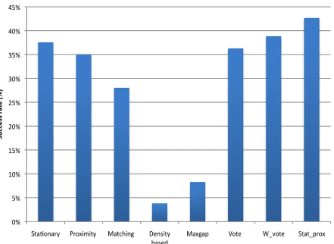
Our approach performs fairly well for the Geolife dataset as the achieved success rate is between 35% and 45% for the stat-prox de-anonymizer (Figure 7). In order to further validate the approach, we applied it on the Nokia dataset. This dataset has 195 users, among which we can generate a “valid” MMC composed of more than one POI for 157 users using the parameters described previously. As shown on Figure 9, the success rate varies between 35% and 42%, with the best score obtained again by the stat-prox de-anonymizer.

0%   5%   10%   15%   20%   25%   30%   35%   40%   45%  

Sta,onary   Proximity     Matching     Density  

based   Maxgap   Vote     W_vote   Stat_prox  

Su cc es s   ra te  (%)      

Figure 9: Success rate of the de-anonymizers on the Nokia dataset.

6.4. Fair comparison with prior work

In this section, we have presented various experiments on de-anonymization attacks that lead to the definition of an heterogeneous de-anonymizer called stat-prox, which obtains a success rate between 42% and 45% on different datasets. While at first glance, this performance may seem to be poorer than the one achieved by the predictors of Ma et al. [16], which goes up to 60% to 90%, and the predictors of Freudiger and co-authors [17] that have a re-identification rate of70%, we believe that these results are not directly comparable because we clearly differentiate between the training set and the testing set, while these authors perform the learning and the testing on the same dataset, thus inducing a strong experimental bias.

Indeed, our mobility models are built out of the training set, which is disjoint from the test set, whereas one of the adversary model of Ma et al. directly extracts mobility traces forming the test set from the training set. Moreover in our case, the training data is temporally separated from the test data (i.e., the training and the test have been recorded at different non-overlapping periods of time) because the whole dataset has been split into two temporally disjoint parts, whereas the second adversary model of Ma et al. picks the information it uses to de-anonymize within the same period as the test data is recorded. Therefore, our approach is quite different from them as our attack consists first in collecting mobility data from an individual, before trying to identify this individual in a so-called anonymized dataset, while their attack aims at gathering location data at the same time at which the de-anonymization attack occurs. In addition, one important parameter of their attack is the number of timestamped location data collected, which can be compared to the number of states we have in our mobility model. On average and depending on the dataset considered, we have between 4 and 8 states per MMC, which correspond to a compact representation of the mobility behavior of an individual. When restricted to such limited of information in terms of the number of timestamped location data, the attacks proposed by Ma et al. do not perform well, with a de-anonymization rate between 10% to 40%. Similarly in the work of Freudiger and co-authors, mobility samples are taken from home/work, POIs or frequent visited places without any distinction between training or testing sets, which again introduces an evaluation bias. For instance, when 90% of the samples are taken either from home or work, the success rate of the re-identification is around 75% while a uniform random sampling leads to a success rate for the re-identification of 10%.

For comparison purpose, we conducted the de-anonymization attack without separating the training and testing sets. The results obtained by related work and for the stat-prox de-anonymizer in this setting using different datasets are summarized in Figure 10. These experiments are, as expected, so biased that they lead to a success rate close to 100% for all the datasets. Once again, we do not pretend that our de-anonymization attack would achieve a success rate of nearly 100% and beat all the previous methods if tested in the same conditions (for instance in some settings the test set was only a subset of the training set as it was sampled from it). We are merely pointing out that for fairness issues, it is important to compare de-anonymizers using the same setting and that in order to reduce the experimental bias, the training and testing set should be clearly separated (which is not the case in almost all the previous works).

0%   10%   20%   30%   40%   50%   60%   70%   80%   90%   100%   ARUM                                                        

(5  users)   (113  users)  GeoLife                                                  (161  users)  Nokia                                                      San  Francisco  Cabs                (137  users)   (24  users)  Borlange                                                        

Stat-­‐prox   Freudiger  et  al.   Ma  et  al.  

Figure 10: Success rate of the stat-prox de-anonymizer when the training and testing sets are the same.

7. Conclusion

In recent years, several privacy breaches related to location data have reached the headlines. For instance, the German deputy Malte Spitz sued Deutsche Telekom to obtain the last six months of location data generated from his phone [34]. Then, he published this data in the form of an interactive map showing that the combination of location data with contextual information could lead to a serious privacy breach. Another example of privacy buzz was the article about telephone constructors [35] published in The Wall Street Journal revealing that Apple and Google collect on a large scale location data using unique identifiers in order to develop novel location-based services.

The classical argument used by data collectors use is that by itself location data is anonymous and thus can be collected from users without violating their privacy. Unfortunately, as shown by our work in this paper this argument is fallacious. More precisely, we have demonstrated that geolocated datasets gathering the movements of individuals are particularly vulnerable to a form of inference attack called the de-anonymization attack. More precisely, we have shown that the de-anonymization attack can re-identify with a high success rate the individuals whose movements are contained in an anonymous dataset provided that the adversary can used as background information some mobility traces of the same individuals that he has been able to observe during the training phase. From these traces, the adversary can build a MMC that models in a compact and precise way the mobility behavior of an individual. We designed novel distances quantifying the similarity between two MMCs and we described how these metrics can be combined to build de-anonymizers. The de-anonymization attack is very accurate with a success rate of up to 45% on large-scale real datasets and this even if the mobility traces are sanitized by downsampling them (e.g., every 2 minutes instead of every 10 seconds).

In summary, the mobility behavior of an individual is far from being random [9] and tends to be unique thus acting as a signature of an individual [27]. For instance, even the pair home/work could act as a quasi-identifier [7]. In addition to location data, the knowledge of the social network, as shown by the works of Srivatsa and Hicks and Sharad and Danezis, can be used as side information to help in performing the de-anonymization. However, it might be possible to mitigate this risk of re-idenfication by sanitizing the social graph before releasing it [36].

In the future, we are planning to extend the current work by following several avenues of research. For instance, one of our research objective is to discover among different clustering algorithms, the one that best fits our needs while being also robust with respect to small changes in the inputs (e.g., small spatial and temporal perturbation). In a different direction, we will also explore how more complex geo-sanitization mechanisms, such as spatial cloaking techniques [37] or mix zones [38], can help to reduce the success rate of the de-anonymization attack.

References

[1] M. Piorkowski, N. Sarafijanovic-Djukic, M. Grossglauser, CRAWDAD data set epfl/mobility (v. 2009-02-24), Downloaded from http://crawdad.cs.dartmouth.edu/epfl/mobility (February 2009).