HAL Id: hal-01511903
https://hal.archives-ouvertes.fr/hal-01511903
Submitted on 21 Apr 2017
HAL is a multi-disciplinary open access
archive for the deposit and dissemination of
sci-entific research documents, whether they are
pub-lished or not. The documents may come from
teaching and research institutions in France or
abroad, or from public or private research centers.
L’archive ouverte pluridisciplinaire HAL, est
destinée au dépôt et à la diffusion de documents
scientifiques de niveau recherche, publiés ou non,
émanant des établissements d’enseignement et de
recherche français ou étrangers, des laboratoires
publics ou privés.
Sylvain Cussat-Blanc, Jean Disset, Stephane Sanchez
To cite this version:
Sylvain Cussat-Blanc, Jean Disset, Stephane Sanchez. Dangerousness Metric for Gene Regulated Car
Driving. 19th European Conference on the Applications of Evolutionary Computation
(EvoApplica-tions 2016), part of EvoStar 2016, Mar 2016, Porto, Portugal. pp. 620-635. �hal-01511903�
Open Archive TOULOUSE Archive Ouverte (OATAO)
OATAO is an open access repository that collects the work of Toulouse researchers and
makes it freely available over the web where possible.
This is an author-deposited version published in :
http://oatao.univ-toulouse.fr/
Eprints ID : 17068
The contribution was presented at EvoApplications 2016 :
http://www.evostar.org/2016/cfp_evoapps.php
To cite this version :
Cussat-Blanc, Sylvain and Disset, Jean and Sanchez,
Stephane Dangerousness Metric for Gene Regulated Car Driving. (2016) In:
19th European Conference on the Applications of Evolutionary Computation
(EvoApplications 2016), part of EvoStar 2016, 30 March 2016 - 1 April 2016
(Porto, Portugal).
Any correspondence concerning this service should be sent to the repository
administrator:
[email protected]
Gene Regulated Car Driving
Sylvain Cussat-Blanc, Jean Disset, and St´ephane Sanchez
University of Toulouse - IRIT - CNRS - UMR5505 21 all´ee de Brienne, 31042 Toulouse, France
{cussat, disset, sanchez}@irit.fr
Abstract. In this paper, we show how a dangerousness metric can be used to modify the input of a gene regulatory network when plugged to a virtual car. In the context of the 2015 Simulated Car Racing Cham-pionship organized during GECCO 2015, we have developed a new car-tography methodology able to inform the controller of the car about the incoming complexity of the track: turns (slipperiness, angle, etc.) and bumps. We show how this dangerousness metric improves the results of our controller and outperforms other approaches on the tracks used in the competition.
Keywords: Gene regulatory network, virtual car racing, dangerousness measure
1
Introduction
The Simulated Car Racing competition (SCR1) aims to design a controller in
order to race competitors on various unknown tracks. This competition is based on The Open-source Racing Car Simulator (TORCS2). Both scripted and
evo-lutionary approaches can be used to control the virtual car. Within the frame of the 2015 competition that was held during GECCO2015, we have improved the approach based on gene regulation evolved with a genetic algorithm firstly presented at the previous edition in 2013 [21]. The SCR competition involves vir-tual car driver competing on 12 tracks, each of them having different properties (shape, track adherence, etc.). The virtual drivers can be hand-written scripts, optimized scripts or learning agents. For each track, the competitors first run alone for 5 laps (warm-up) during which they can learn the track. Then, the competitors run for a qualifying session during which they have to race against the clock in 5 laps. This qualifying session determines the starting order of the final round: the race. During this stage, all the competitors are running at the same time for 5 laps. The competitors are evaluated on this race based on the Formula One point system. The championship is composed of 12 of these races and the winner is the driver with the maximum number of points.
1
http://cs.adelaide.edu.au/∼optlog/SCR2015/index.html 2
Amongst the existing controllers for virtual car racing games that use an evo-lutionary process to optimize the driver behavior, we can broadly consider two kind of controllers. The first kind are indirect controllers where the inputs are not directly linked to the outputs of the virtual racing car. The inputs are com-puted and transmitted to driving policies based on hand-coded rules or heuristics that manage steering and throttle controls. Usually, these controllers optimize their driving policies with an evolutionary algorithm [4,18,19]. These kind of controllers are efficient and they have been at the top of the SRC competition since 2009. The second kind of controllers are direct controllers where sensors are directly mapped to the car effectors. These direct controllers actually learn how to drive the car using its sensors and actuators. They can be based on evolved artificial neural networks [24,2,23,22,5] or genetic programming [1]. These meth-ods usually produced either very fast controllers but specialized on one specific track or slower more generic drivers. Because evolving a direct controller from scratch that can drive on-track and manage all car controls and race events is difficult, these controllers are sometimes mixed with hand-coded policies that modify the controller outputs to handle crash recovery or opponents, or that manage specific controls such as gear handling.
The controller we develop is a direct controller. Instead of designing complex hand-coded heuristics, we prefer to evolve the controller to drive the car by using a standard genetic algorithm. In this work, the controller is based on a Gene Regulatory Network (GRN). In order to optimize this GRN, we have used an incremental evolution (as in [24,4]) based on different fitnesses that gradually refine the controller’s behavior. The improvement we detail in this paper is related to the first stage (warm-up) but it impacts the behavior of the driver on both other stages. It consists in modifying the GRN inputs depending on an on-the-fly dangerousness measure of the track. Based on that, the GRN modify its behavior in order to slow down or speed up based on the current situation of the car (position on the track, sliding of the car, etc.).
The paper is organized as follows. Section 2 presents gene regulatory networks in general, describing the existing computational models and the problems they are currently handling. This section also introduces the computational model we have used in this work. Section 3 summarizes how the GRN is connected to the car sensors and actuators and how the GRN is incrementally trained with a genetic algorithm to produce a basic driver. Then, section 4 details our learning approach of the tracks, the dangerousness measure we produce and how it influences the inputs of the gene regulatory network. Section 5 proposes an experimental validation of our approach by evaluating the GRNDriver with and without the dangerousness measure against the drivers involved in the 2015 edition of the SCR competition.
2
Gene regulatory network
Gene Regulatory Networks (GRN) are biological structures that control the in-ternal behavior of living cells. They regulate gene expression by enhancing and
inhibiting the transcription of certain parts of the DNA. For this purpose, the cells use protein sensors dispatched on their membranes; these provide crucial information to guide the cells through their cycle. Many modern computational models of these networks exist. They are used both to simulate real gene regu-latory networks [20,3,11] and to control agents [10,12,17,14].
When used for simulation purpose, a GRN is usually encoded within a bit string, as DNA is encoded within a nucleotide string. As in real DNA, a gene sequence starts with a particular sequence, called the promoter in biology [16]. In the real DNA, this sequence is represented with a set of four protein: TATA where T represents the thymine and A the Adenine. In [20], Torsten Reil is one of the first to propose a biologically plausible model of gene regulatory networks. The model is based on a sequence of bits in which the promoter is composed of the four bits 1010. The gene is coded directly after this promoter whereas the regulatory elements are coded before the promoter. To visualize the properties of these networks, he uses graph visualization to observe the concentration vari-ation of the different proteins of the system. He points out three different kinds of behavior from randomly generated gene regulatory networks: stable, chaotic and cyclic. He also observes that these networks are capable of recovering from random alterations of the genome, producing the same pattern when they are randomly mutated. In 2003, Wolfgang Banzhaf formulates a new gene regulatory network heavily inspired from biology [3]. He uses a genome composed of mul-tiple 32-bit integers encoded as a bit string. Each gene starts with a promoter coded by any integer ending with the sequence “XYZ01010101”. This sequence occurs with a 2−8 probability (0.39%). The gene following this promoter is then
coded in five 32-bits integers (160 bit) and the regulatory elements are coded upstream to the promoter by two integers, one for the enhancing and one for the inhibiting kinetics. Banzhaf’s model confirms the hypothesis pointed out by Reil’s one; the same properties emerges from his model.
From these seminal models, many computational models have been initially used to control the cells of artificial developmental models [11,10,14]. They sim-ulate the very first stage of the embryogenesis of living organisms and more particularly the cell differentiation mechanisms. One of the initial problem of this field of research is the French Flag problem [26] in which a virtual organism has to produce a rectangle that contains three strips of different colors (blue, white and red). This simulates the capacity of differentiation in a spatial environ-ment of the cells. Many models addressed this benchmark with cells controlled by a gene regulatory network [15,14,6]. More recently, gene regulatory networks have proven their capacity to regulate complex behaviors in various situations: they have been used to control virtual agents [17,13,9] or real swarm or modular robots [12,8].
2.1 Our model
The gene regulatory network used to control a virtual car in this work is based on Banzhaf’s model. It has already been successfully used in other applications.
It is capable of developing modular robot morphologies [8], controlling cells de-signed to optimize a wind farm layout [25] and controlling reinforcement learning parameters in [7]. This model has been designed for computational purpose only and not to simulate a biological network.
This model is composed of a set of abstract proteins. A protein a is composed of three tags:
– the protein tag ida that identifies the protein,
– the enhancer tag enha that defines the enhancing matching factor between
two proteins, and
– the inhibitor tag inha that defines the inhibiting matching factor between
two proteins.
These tags are coded with an integer in [0, p] where the upper bound p can be tuned to control the precision of the network. In addition to these tags, a protein is also defined by its concentration that will vary over time with particular dynamics described later. A protein can be of three different types:
– input, a protein whose concentration is provided by the environment, which regulates other proteins but is not regulated,
– output, a protein with a concentration used as output of the network, which is regulated but does not regulate other proteins, and
– regulatory, an internal protein that regulates and is regulated by others pro-teins.
With this structure, the dynamics of the GRN are computed by using the protein tags. They determine the productivity rate of pairwise interaction be-tween two proteins. For this, the affinity of a protein a for another protein b is given by the enhancing factor u+ab and the inhibiting factor u−abcalculated as follows:
u+ab= p − |enha− idb| ; u−ab= p − |inha− idb| (1)
The proteins are then compared pairwise according to their enhancing and inhibiting factors. For a protein a, the total enhancement ga and inhibition ha
are given by: ga= 1 N N X b cbeβu + ab−u + max ; h i= 1 N N X b cbeβu − ab−u−max (2)
where N is the number of proteins in the network, cb is the concentration of
the protein b, u+
max is the maximum observed enhancing factor, u−max is the
maximum observed inhibiting factor and β is a control parameter which will be detailed hereafter. At each timestep, the concentration of a protein a changes with the following differential equation:
dca
dt =
δ(ga− ha)
where Φ is a normalization factor to ensure that the total sum of the output and regulatory protein concentrations is equal to 1. β and δ are two constants that influence the reaction rates of the network. β affects the importance of the matching factors and δ is used to modify the production level of the proteins in the differential equation. In summary, the lower both values are, the smoother the regulation is; the higher the values are, the more sudden the regulation is.
3
Using a GRN to drive a virtual car
3.1 Linking the GRN to the car sensors and actuators
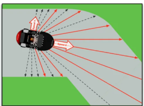
The GRN can be seen as any kind of computational controller: it computes inputs provided by the problem it is applied to and it returns values to solve the problem. To use the gene regulatory network to control a virtual car, our main wish is to keep the connection between the GRN and the car sensors and actuators as simple as possible. In our opinion, the approach should be able to handle the reactivity necessary to drive a car, the possible noise of the sensors and unexpected situations. The car simulator provides 18 track sensors spaced 10◦ apart and many other sensors such as car fuel, race position, motor speed,
distance to opponents, etc. However, in our opinion, all of the sensors are not required to drive the car. Reducing the number of inputs directly reduces the complexity of the GRN optimization. Therefore, we have selected the following subset of sensors provided by the TORCS simulator:
– 9 track sensors that provide the distance to the track border in 9 different directions,
– longitudinal speed and transversal speed of the car.
Figure 1 represents the sensors used by the GRN to drive the car. Before being computed by the GRN, each sensor value is normalized to [0, 1] with the following formula:
norm(v(s)) = v(s) − mins maxs− mins
(3) where v(s) is the value of sensor s to normalize, minsis the minimum value of
the sensor and maxs is the maximum value of the sensor.
Once the GRN input protein concentrations are updated, the GRN’s dy-namics are run one time in order to propagate the concentration modification to the whole network. The concentrations of the output proteins are then used to regulate the car actuators. Four output proteins are necessary: two proteins oland or for steering (left and right), one protein oafor the accelerator and one
Speed X Sp e e d Y 31 3131313131 GRN Driver GRN Driver
Fig. 1: Sensors of the car connected to the GRN. The red plain arrows are used track sensors whereas the gray dashed ones are the track sensors also available in the simulator but not used by the GRN. The plain arrows Speed X and Speed Y are respectively the longitudinal and the transversal car speeds.
3.2 GRN genome
Before it can drive, the regulatory network needs to be optimized. In this work, we use a standard genetic algorithm to optimize the GRN’s protein tags, en-hancing tags and inhibiting tags. The GRN can be easily encoded in a genome. The genome contains two independent chromosomes. The first one is defined as a variable length chromosome of indivisible proteins. Each protein is encoded with three integers between 0 and p that correspond to the three tags. In this particular work, p is set at 32 and the genome proteins are organized with the input proteins first, followed by the output proteins and then regulatory pro-teins. The inputs and outputs presented in the previous section will be always be linked to the same protein.
This chromosome requires particular crossover and mutation operators: – a crossover can only occur between two proteins and never between two tags
of the same protein. This ensures the integrity of both subnetworks when the GRN is subdivided into two networks. When assembling another GRN, local connections are kept with this operator and only new connections between the two networks are created.
– three mutations can be equiprobably used: add a new random regulatory protein, remove one protein randomly selected in the set of regulatory pro-teins, or mutate a tag within a randomly selected protein.
A second chromosome is used to evolve the dynamics variables β and δ. This chromosome consists of two double-precision floating point values and uses the standard mutation and crossover methods. These variables are evolved in the in-terval [0.5, 2]. Values under 0.5 produce unreactive networks whereas values over 2 produce very unstable networks. These values are chosen empirically through a series of test cases.
3.3 Incremental evolution
In order to optimize the GRN to drive a car, we use an incremental evolution in three stages3. This section summarizes these three stages. More details can be
found in [21].
The first stage consists of training the GRN to drive as far as possible, with a minimum speed, on one track. We use CGSpeedway, which is simple with long turns and straight lines. Each tested GRNDriver is rewarded when going farther and faster with an innovative ticket system. The ticket represents the maximum time the GRNDriver must take to cover a sector of a certain distance. Furthermore, the ticket’s value is reduced each time the GRNDriver validates a sector: the farther the GRN goes on the track, the faster it must drive. The
3
During these stages, the same parameters have been used to tune the genetic algo-rithm. Only the fitness function is modified. The genetic algorithm parameters are: Population size: 500; Mutation rate: 15%; Crossover rate: 75%; GRN Size: [4, 20] regulatory proteins plus inputs and outputs.
fitness is given by the distance covered by the GRNDriver without getting out of the track or getting out of time on a sector. This first stage builds a basic network with which the GRNDriver can drive endlessly on this particular track. It can also drive on most of the tracks but hard turns, never encountered in CGSpeedway, are still problematic.
In order to generalize the network to any possible track, we evolved the previous GRN a second time with the same evolutionary process but on three different tracks. The tracks used are CGSpeedway (in order not to lose the driving capabilities of the previous GRN), Alpine and Street. The fitness function is the sum of the fitnesses of the first evolution stage successively applied to the three tracks. At the end of this evolution, the best GRN is able to drive on every possible track. It drives very safely, going at a suitable speed to go through every kind of turn and braking when it detects a turn.
The final stage of evolution consists in removing all possible imperfection of the best GRN obtained previously. We observed a few oscillatory behavior, very common with GRNs, that could be a problem in a racing car championship. To minimize the oscillatory behaviors, we evolve the best GRN one last time. This time we add to the fitness function another test case that penalizes the continuous oscillations of the car on straight lines and long turns or fast multiple steering changes from full right to full left. As with the ticket system used in the previous fitness functions, we simply stop the evaluation if we detect oscillatory behaviors.
4
Influencing the GRN with a dangerousness measure
In order to make the previously evolved GRN fast enough to win a car racing competition, we have designed a dangerousness measure that allows the GRN to anticipate the incoming complexity of the track. This measure needs a full cartography (turns, slipperiness, etc.) of the track and modify the longitudinal speed input of the GRN. This sections details these two parts.
4.1 Track cartography
The cartography consists in recording a maximum of information about a track during one lap. Therefore, we have scripted a driver that strictly follows the middle of the track at a limited speed of 90km/h. To do so, the behavior is decomposed as follows:
– Steering wheel. The angle of the wheel is given by the angle of the car with the track: if the car longitudinal axis is not aligned with the track tangent, the car driver must turn the wheel in the corresponding direction. This wheel angle direction is corrected with the track position in order to avoid any possible derivation of the car: if the car is shifted to the left (respectively right) hand side of the track, the wheel angle is augmented (respectively reduced) in order to recenter the car.
– Gas and brake pedals. The gas/brake pedals are regulated so that the car speed stay as close as possible to the target speed. To do so, the following formulas are used to compute the gas pedal value g and the brake pedal value b: g = max(0, th) (7) b = min(0, −th) with th = 2 1 + exp(sc− st) − 1 where sc is the car current speed, stis the target speed.
This simple cartographic driver has been made so that the car can pass through all possible curves fast enough to produce some transversal speed (slides). This is important in order to evaluate in each turn the quality of the track and therefore the speed limits of the car. While driving, the script identifies track sectors according to the wheel angle and Z-axis speed. Sectors can be of following types:
– left if the left front sensor is greater than the right front sensor and actual steering is greater than 0.025rad (steering left),
– right if the right front sensor is greater than the left front sensor and actual steering is smaller than -0.025rad (steering right),
– jump if the Z-axis speed is smaller than -12.5km/h, – straight otherwise.
At each time step of the cartography, a new sector is created when the sector type is different to the sector type at the previous time step. This allows subdivision of the tracks to as a series of sectors. In each sector, the following values are stored:
– the sector length ls,
– sum of transversal speeds sy,
– sum of Z-axis speeds sz,
– sum of wheel angles wa.
With these data, two dangerousness measures are calculated for each sectors: – the turn dangerousness, which expresses the turn complexity, given by |wa−sy| ls ,
– the jump dangerousness, which expresses the jumping risk of the car, given by 50|sz|
ls .
These measures are used by the GRN to regulate its speed before and during the turn. Before being used by the GRN, the track cartography is first filtered in order to remove micro sectors generated by sensor noise. To do so, all straight sectors which length is smaller than 50 meters are removed. Their data are reallo-cated to the neighbor sectors and their dangerousness measures are recalculated. The turn dangerousness measure is refined during the 4 last laps of the warm-up and the qualifying session in order to eliminate all possible risk of accident.
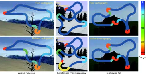
0 800 400 200 600 + Danger
Wildno-mountain Limalonges-mountain-snow Makiewec-hill
Raw cartography
Refined cartography Refined cartography Raw cartography
Raw cartography
Refined cartography
Fig. 3: Examples of cartographies obtained, before refining (upper figures) and after (lower ones).
When the GRNDriver gets off the track, the dangerousness value of the sector is increased so that the same mistake is avoided during the next laps. Figure 3 shows both the turn dangerousness measure obtained right after the cartography stage (upper figures) and the refined cartographies at the end of the qualifying session (lower figures). We can observe that the refining is necessary in some turns, under evaluated by the initial cartography (first two tracks: Wildno and Limalonges). In particular, this is necessary after long straights to build a braking zone which cannot appear with the low speed of the driver during cartography. 4.2 Influence on the GRN inputs
In order to regulate the GRNDriver speed, we have decided to distort the car longitudinal speed sensor. Whereas most other approaches manipulated directly the output of the controller, we have decided to modify its input so that the GRNDriver keeps full control of the situation based on its full perceptions. For example, even if the dangerousness measure is low, the GRN can decide not to accelerate because the current car state is unstable (the car could be sliding, on a bad track position, etc.). To distort the longitudinal speed sensor, a speed regulator coefficient is applied to the direct sensor value. The aim of the coeffi-cient is to let the GRN think the car is going slower than it really does when the dangerousness is low and faster when the dangerousness is high. This encourages the GRN either to speed up or slow down the car. To do so, the GRNDriver uses the incoming sectors (including the one it is currently in) up to the sector at a distance of 0.002 ∗ s2
x, where sxis the current longitudinal speed. This allows the
GRNDriver to regulate the dangerousness estimation according to the car speed. With these sectors, the turn dangerousness dt and the jump dangerousness dj
Based on the global dangerousness, different cases scenarios are identified to compute the speed regulator coefficient Cs:
Cs= 0.5 if si is straight and dg< tn
0.66 if si is not straight and dg< tl
0.66 if si is not straight, dg< th and dist(si) > 0.37 ∗ ls
2 if si is not straight, dg< tm, sx> 135km/h and dist(si+1) < s2x/700
2 if si+1 is jump,sx> 170 and dist(si+1) < s2x/800
5 if si is straight, dg> th, sx> 120km/h and dist(si+1) < s2x/600
5 if si is straight, dg< th, sx> 135km/h and dist(si+1) < s2x/850
0.9 otherwise
(8) where
– si is the current sector and si+1is the next sector,
– dg is the current global dangerousness,
– tn= 150 is the no dangerousness threshold, tl= 250 is the low dangerousness
threshold, tm= 400 is the medium dangerousness threshold and th= 800 is
the high dangerousness threshold,
– dist(si) (resp. dist(si+1) is the distance to the beginning of the current (resp.
next) sector,
– sx is the car current longitudinal speed.
In these formulas, the condition dist(si+1) < s2x/y, with y = 600, 700, 800 or 850,
is used to evaluate the braking distance necessary to speed the car down to the target speed. All the parameters involved in this formula have been empirically chosen through test. A broader study could improve the approach and its results. This speed regulator coefficient Csis then simple multiplied to the car
lon-gitudinal speed sx to provide the car speed input c(iSx) of the GRN:
c(iSx) = norm(sx∗ Cs) (9)
This input is sufficient to modify because it is strongly linked to the acceleration output protein: other proteins are too (such as the front track sensor) but are harder to modify due to their implications in the driving. Modifying a track sensor might generate bad behavior when the GRNDriver is sliding in a turn for example. The modification of the car speed input seams to be the more direct and efficient way to impact the GRNDriver speed behavior.
5
Comparative study
In order to evaluate the dangerousness measure approach, we have compared its benefits on the GRNDriver to other approaches submitted to the competition4
4
The source code and a short description of these approaches are available on the competition website: http://cs.adelaide.edu.au/∼optlog/SCR2015/
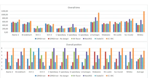
!"!! #!!"!! $!!"!! %!!"!! &!!"!! '!!!"!! '#!!"!! ()*+,-.# /01,2-3453 6+07.' 6+07.8 9.:*--2;4< =.>*--2;4< ?.>*--2;4< @+A4)1,B-> C4D1;+-5 E,.54>7)- :55.7045D# F+)2,1
GH-04))I7+A-?JE60+H-0 ?JE60+H-0I. E1I24,B-0 C0IJ45-0 E--2$:: :,4D-G+) =9.:J9
! " # $ % & '
()*+,-.# /01,2-3453 6+07." 6+07.$ 8.9*--2:4; <.=*--2:4; >.=*--2:4; ?+@4)1,A-= B4C1:+-5 D,.54=7)- 955.7045C# E+)2,1 (F-04A-GF-04))H*1=+7+1,
>ID60+F-0 >ID60+F-0H. D1H24,A-0 B0HI45-0 D--2%99 9,4C-G+) <8.9I8
Fig. 4: The upper plot presents the overall time to cover the 5 laps in qualifying mode. The lower one presents the position of the drivers according to the overall time.
on the 12 tracks used during the competition. With this aim in mind, we have compared the GRNDriver with and without the speed regulator coefficient as well as the other approaches using the first two stage of the competition rules:
1. the drivers are run in warm-up mode during 5 laps in order to learn the track.
2. they are then run in qualifying mode for 5 more laps.
In this comparative study, only the results of the qualifying session are presented. Because the focus of the paper is the dangerousness measure we have introduced this year, the results of the race are not presented in this paper. However, they are also available on competition website. All the runs have been made with noisy sensors.
Figure 4 presents the overall time taken by the competitors to cover 5 laps and their position. Times (upper chart) are very close between competitors and it is hard to evaluate which approach is better than the other. However, when looking to position (lower chart), we can observe that the GRNDriver is most of the time first with the dangerousness measure on and second when switched off. This can be viewed with the last bars labelled “Average” which represent the positions of the drivers averaged over the tracks. The GRNDriver with the dangerousness measure finishes on average 2.25, the GRNDriver without dangerousness measure finishes on average 2.83 and the next closer competitor, Mr. Racer, finishes 3.33. When only comparing the GRNDriver with and without the dangerousness metric, we can observe that the dangerousness measures improve the results of the GRNDriver on 8 out of 12 tracks. The Wildno track seams to be problematic for this approach, the GRNDriver with dangerousness measure having lower
GRNDriver GRNDriver with without dangerousness dangerousness measure measure Lap 1 117.75 88.24 Lap 2 96.25 79.86 Lap 3 102.63 79.82 Lap 4 97.85 80.12 Lap 5 103.04 80.12
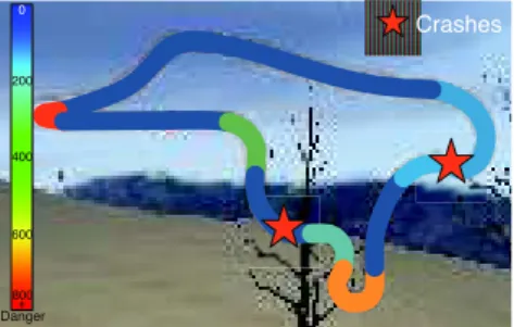
Fig. 5: Lap time of the GRNDriver with and without the dangerousness measure on Wildno. 0 800 400 200 600 + Danger Crashes
Fig. 6: The GRNDriver crashes in two sequences of turns (red stars) when the dangerousness measure is activated because it makes the GRN-Driver braking in a curve.
performances than expected. This bad performance implies a poor ranking on this particular track. Table 5 provides the time of each lap on the Wildno track for the GRNDriver with and without dangerousness measure. The table shows a big instability of the driver over the laps. The GRNDriver with dangerousness measure actually gets out off the track often, which is unproductive. On this particular track the dangerousness measure seams to be too optimistic and makes the car hard to control for the GRN. More precisely, figure 6 shows where the GRNDriver with dangerousness measure crashes on the track: it is always in the middle of a sequence of turns. The dangerousness metric forces the GRN to brake in the turn which leads to a spin. However, the GRNDriver without dangerousness measures finishes the qualifying session in first position (see figure 4). Wildno is a complex mountain track with a complex track to manage: a safe approach of this track looks to be more productive than an aggressive one.
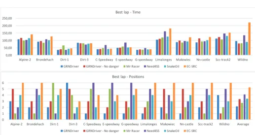
Figure 7 shows the best time of the same 5-laps qualifying session. The bene-fits of the dangerousness measure are here undeniable, the GRNDriver with this feature making 10 times out of 12 better best time than without it. This is an important measure because the best lap corresponds to a lap at the very end of the learning curve of the dangerousness measure. It corresponds to the data that will be used during the race session against other approaches: being faster on one lap is decisive at this point. When looking at the average ranking of the GRN-Driver with and without the dangerousness measure, we observe that enabling it allows the GRNDriver to overtake Mr Racer, which is the closest opponent to the GRNDriver. This shows, in race condition regarding to the cartography of the track, the significance of this feature.
6
Conclusion
In this paper, we have presented an improved version of our learning procedure of a track used to influence the inputs of a gene regulatory network that drives
!"!! #!"!! $!!"!! $#!"!! %!!"!! %#!"!! &'()*+,% -./*0+1231 4).5,$ 4).5,6 7,8(++092: ;,<(++092: =,<(++092: >)?2'/*@+< A2B/9)+3 C*,32<5'+ 833,5.23B% D)'0*/ -+<5E '2(E, F)?+
=GC4.)H+. =GC4.)H+.E, C/E02*@+. A.EG23+. C++0I88 8*2B+J)' ;7,8G7
! " # $ % & '
()*+,-.# /01,2-3453 6+07." 6+07.$ 8.9*--2:4; <.=*--2:4; >.=*--2:4; ?+@4)1,A-= B4C1:+-5 D,.54=7)- 955.7045C# E+)2,1 (F-04A-/-=7G )4*G. H1=+7+1,=
>ID60+F-0 >ID60+F-0G. D1G24,A-0 B0GI45-0 D--2%99 9,4C-J+) <8.9I8
Fig. 7: The upper plot presents the best time of the 5-laps qualifying session. The lower one presents the position of the drivers according to the best lap.
a simulated racing car. We have designed a dangerousness metric that evaluates the dangerousness of the track and helps the GRN to regulate the car speed in function of the turn difficulties (slipperiness, angle, etc.) and the possible jumps due to track bumps. We show the quality of this metric by comparing the GRNDriver with and without its influence on the 12 tracks used in the Simulated Car Racing Championship. In particular, we show that it greatly improves the best lap time of the GRNDriver, which is crucial when opposed to other drivers during a race session. At the end, the GRNDriver won the 2015 edition of the SCRC both because of the generalization capacity of the GRN (able to drive fast on any kind of track with no re-optimization) and because of the improvement brought by the dangerousness method.
To improve this work, multiple options have to be investigated. Our goal is to design a driver with as much automatic learning as possible. First, the use of the GRN as a racing driver requires the design of a track learning method to speed up the wise GRNs we generally obtain by evolution. We would like to teach the GRN to go faster by the use of a hierarchical architecture: a second GRN, pre-optimized on multiple tracks and reoptimized during the warm-up stage, could modify the inputs and/or the outputs of the driving GRN according to the current car state. The specialization capacity of the GRN observed in the first evolutionary step could be helpful during this warm-up stage.
This GRNDriver must also be improved in order to correctly handle oppo-nents. For now, the perception of the GRN is modified by a hand-written script in order to overtake or avoid an opponent detected to close to the car. This approach is innovative in comparison to most other approaches because they usually directly impact the car actuators. Modifying the inputs instead of the output keeps the controller as the center piece of the algorithm. However, we
want the GRN to learn to handle this move by itself because most overruns are currently due to this script. Having all the information the car can detect and letting the GRN decide the best move could reduce this issue.
The application of such an approach to a real car driving is still problem-atic because of the difficulty to prove the security of this approach: in order to drive a real car, it is necessary to strictly prove the algorithm. It is currently mathematically complex to make it on a gene regulatory network because of the complexity of the generated network. However, this approach could be exploited as a controller in a car racing game: multiple GRNs could evolve in parallel with the player, making non-scripted controllers with a large diversity. It could improve the interest of the game by producing different strategies to which the player would have to face.
References
1. A. Agapitos, J. Togelius, and S. M. Lucas. Evolving controllers for simulated car racing using object oriented genetic programming. In Proceedings of the 9th an-nual conference on Genetic and evolutionary computation, pages 1543–1550. ACM, 2007.
2. C. Athanasiadis, D. Galanopoulos, and A. Tefas. Progressive neural network train-ing for the open ractrain-ing car simulator. In Computational Intelligence and Games (CIG), 2012 IEEE Conference on, pages 116–123. IEEE, 2012.
3. W. Banzhaf. Artificial Regulatory Networks and Genetic Programming. In R. L. Riolo and B. Worzel, editors, Genetic Programming Theory and Practice, chapter 4, pages 43–62. 2003.
4. M. V. Butz and T. D. L¨onneker. Optimized sensory-motor couplings plus strategy extensions for the torcs car racing challenge. In Proceedings of the 5th international conference on Computational Intelligence and Games, CIG’09, pages 317–324, Pis-cataway, NJ, USA, 2009. IEEE Press.
5. L. Cardamone, D. Loiacono, and P. L. Lanzi. Learning to drive in the open racing car simulator using online neuroevolution. Computational Intelligence and AI in Games, IEEE Transactions on, 2(3):176–190, 2010.
6. S. Cussat-Blanc, N. Bredeche, H. Luga, Y. Duthen, and M. Schoenauer. Artificial gene regulatory networks and spatial computation: A case study. In Proceedings of the European Conference on Artificial Life (ECAL’11). MIT Press, Cambridge, MA, 2011.
7. S. Cussat-Blanc and K. Harrington. Genetically-regulated neuromodulation facili-tates multi-task reinforcement learning. In Proceedings of the 2015 on Genetic and Evolutionary Computation Conference, pages 551–558. ACM, 2015.
8. S. Cussat-Blanc and J. Pollack. Cracking the egg: Virtual embryogenesis of real robots. Artificial life, 20(3):361–383, 2014.
9. S. Cussat-Blanc, S. Sanchez, and Y. Duthen. Simultaneous cooperative and con-flicting behaviors handled by a gene regulatory network. In Evolutionary Compu-tation (CEC), 2012 IEEE Congress on, pages 1–8. IEEE, 2012.
10. R. Doursat. Organically grown architectures: Creating decentralized, autonomous systems by embryomorphic engineering. Organic Computing, pages 167–200, 2008. 11. P. Eggenberger Hotz. Combining developmental processes and their physics in an artificial evolutionary system to evolve shapes. On Growth, Form and Computers, page 302, 2003.
12. H. Guo, Y. Meng, and Y. Jin. A cellular mechanism for multi-robot construc-tion via evoluconstruc-tionary multi-objective optimizaconstruc-tion of a gene regulatory network. BioSystems, 98(3):193–203, 2009.
13. M. Joachimczak and B. Wr´obel. Evolving Gene Regulatory Networks for Real Time Control of Foraging Behaviours. In Proceedings of the 12th International Conference on Artificial Life, 2010.
14. M. Joachimczak and B. Wr´obel. Evolution of the morphology and patterning of artificial embryos: scaling the tricolour problem to the third dimension. In Advances in Artificial Life. Darwin Meets von Neumann, pages 35–43. Springer, 2011. 15. J. Knabe, M. Schilstra, and C. Nehaniv. Evolution and morphogenesis of
differ-entiated multicellular organisms: autonomously generated diffusion gradients for positional information. Artificial Life XI, 11:321, 2008.
16. R. Lifton, M. Goldberg, R. Karp, and D. Hogness. The organization of the histone genes in drosophila melanogaster: functional and evolutionary implications. In Cold Spring Harbor symposia on quantitative biology, volume 42, pages 1047–1051. Cold Spring Harbor Laboratory Press, 1978.
17. M. Nicolau, M. Schoenauer, and W. Banzhaf. Evolving genes to balance a pole. In A. I. Esparcia-Alcazar, A. Ekart, S. Silva, S. Dignum, and A. S. Uyar, editors, Proceedings of the 13th European Conference on Genetic Programming, EuroGP 2010, volume 6021 of LNCS, pages 196–207, 2010.
18. E. Onieva, D. A. Pelta, J. Alonso, V. Milan´es, and J. P´erez. A modular paramet-ric architecture for the torcs racing engine. In Proceedings of the 5th international conference on Computational Intelligence and Games, CIG’09, pages 256–262, Pis-cataway, NJ, USA, 2009. IEEE Press.
19. J. Quadflieg, M. Preuss, and G. Rudolph. Driving faster than a human player. In Proceedings of the 2011 international conference on Applications of evolutionary computation-Volume Part I, pages 143–152. Springer-Verlag, 2011.
20. T. Reil. Dynamics of gene expression in an artificial genome-implications for bio-logical and artificial ontogeny. Lecture notes in computer science, pages 457–466, 1999.
21. S. Sanchez and S. Cussat-Blanc. Gene regulated car driving: using a gene regulatory network to drive a virtual car. Genetic Programming and Evolvable Machines, 15(4):477–511, 2014.
22. K. Stanley, R. Sherony, N. Kohl, and R. Miikkulainen. Neuroevolution of an auto-mobile crash warning system. In In Proceedings of the Genetic and Evolutionary Computation Conference (GECCO), 2005.
23. K. O. Stanley and R. Miikkulainen. Evolving neural networks through augmenting topologies. Evolutionary Computation, 10, 2002.
24. J. Togelius and S. M. Lucas. Evolving robust and specialized car racing skills. In Evolutionary Computation, 2006. CEC 2006. IEEE Congress on, pages 1187–1194. IEEE.
25. D. Wilson, E. Awa, S. Cussat-Blanc, K. Veeramachaneni, and U.-M. O’Reilly. On learning to generate wind farm layouts. In Proceeding of the fifteenth annual conference on Genetic and evolutionary computation conference, pages 767–774. ACM, 2013.
26. L. Wolpert. Positional information and the spatial pattern of cellular differentia-tion. Journal of theoretical biology, 25(1):1, 1969.