HAL Id: hal-01088626
https://hal-mines-nantes.archives-ouvertes.fr/hal-01088626
Preprint submitted on 28 Nov 2014
HAL is a multi-disciplinary open access archive for the deposit and dissemination of sci-entific research documents, whether they are pub-lished or not. The documents may come from teaching and research institutions in France or
L’archive ouverte pluridisciplinaire HAL, est destinée au dépôt et à la diffusion de documents scientifiques de niveau recherche, publiés ou non, émanant des établissements d’enseignement et de recherche français ou étrangers, des laboratoires
Optimization of customer orders routing in a
collaborative distribution network
Fabien Lehuédé, Olivier Péton, Xin Tang
To cite this version:
Fabien Lehuédé, Olivier Péton, Xin Tang. Optimization of customer orders routing in a collaborative distribution network. 2014. �hal-01088626�
Optimization of customer orders routing
in a collaborative distribution network
´
Ecole des Mines de Nantes Rapport Interne 14/6/AUTO
october 2014
Fabien Lehu´ed´e, Olivier P´eton, Xin Tang ´
Ecole des Mines de Nantes, IRCCyN (UMR CNRS 6597) 4 rue Alfred Kastler, 44300 Nantes, France Tel.: +33-251-858-321 Fax: +33-251-858-349 fabien.lehuede, olivier.peton, [email protected]
Abstract
This paper presents a sequential approach for the assessment of a multi-layered distribution network from a cluster of collaborating suppliers to a large set of cus-tomers. The transportation network includes three segments: suppliers routes from suppliers to a consolidation and distribution center, full truckload routes toward regional distribution centers, and less-than-truckload distribution toward final cus-tomers. In every shipping date, the optimization problem consists of assigning customers to regional distribution centers and determining the routes of vehicles through the whole distribution network. This problem is first modeled as a Mixed Integer Linear Problem (MILP). Then, we propose to decompose it into three smaller MILPs that are solved sequentially in order to quickly provide a good approximate solution. The experiments on real data show that the decomposition method pro-vides near optimal solutions within a few minutes while the original model would require hours of calculation.
Keywords: Horizontal collaboration, mixed integer linear programming, distri-bution network design, load plan
1
Introduction
Horizontal collaboration in a supply chain is characterized by a pooling of resources between manufacturers rather than manufacturers collaborating with logistics service providers or 4PLs (vertical collaboration) [15]. Companies which resort to horizontal collaboration have to overcome many cultural, organizational and technical barriers, among which the fear for information disclosure, the difficulty to establish relationships of trust, the need for new IT tools or legal aspects. Competing companies are often reluctant to share strategic internal resources. External operations such as the supply or distribution of goods are often natural candidates for horizontal collaboration. They
can be easily outsourced and shared with other manufacturers, including competing companies.
Pooling the transportation of goods represents a cost reduction opportunity in two ways. Firstly, Less-Than-Truckload (LTL) shipments of each collaborating company can be consolidated into Full TruckLoad (FTL) shipments, which turns out to be much cheaper. Secondly, whenever FTL shipments are not possible, the cost of LTL consoli-dated shipments is cheaper than small-sized separated shipments, due to economies of scale. From the organizational point of view, collaborative logistics is also a mean to sign long-term partnership agreements with a few reliable Logistic Service Providers (LSP) and to guarantee a regular service, rather than looking for one-shot transportations everyday with multiple carriers. Finally, from the customers point of view, common deliveries instead of several small volume deliveries improve the quality of service.
However, horizontal collaboration comes at various costs and impediments [10]. The first obvious difficulty is the need to synchronize the material flows in order to organize common deliveries. This requires organizing pickup routes between the collaborating companies or to create a shared consolidation center. This new facility induces additional logistics costs and break bulk which did not exist before. In practice, it is very hard to estimate a priori if the cost of collaboration is compensated by the resulting cost reduction. Thus, only non negligible savings are worth the increased system complexity. In this paper, we consider a cluster of companies which aim at establishing horizontal collaboration for the delivery of their goods from one production region to a set of customers spread across a wide area. The main objective of this collaboration is to build pooled load plans that cut expenditure on the distribution costs through volume consolidation. The second objective is to improve the quality of service to customers by synchronizing the deliveries.
A global objective of the paper is to assess a collaborative logistic network composed of one consolidation and distribution center (CDC) and several regional distribution cen-ters (RDC). In particular, one has to check whether a grand coalition, i.e. a coalition in-volving all players, is viable from an economic point of view. For confidentiality reasons, we cannot provide numerical results concerning the quantitative benefits of collabora-tive distribution and the cost allocation mechanism. We rather focus on the modeling of the distribution optimization in the collaborative network and the decomposition of the original model into three subproblems.
The contribution of this paper is two-fold. We propose a mixed integer linear pro-gramming (MILP) modeling for a rich horizontal collaboration case which includes sev-eral layers of facilities, multiple transportation segments and structure costs. Minimizing the cost of daily load plans is difficult due to the variety of all possible material flows through the logistics network and the simultaneous use of FTL and LTL routes with different cost structures. Since the global MILP model is intractable in practice, we propose a decomposition approach which defines three independent subproblems which are solved sequentially. This approach is tested on a real-life case study with 7 suppliers and more than 5000 customers. A computational study evaluate the performance of the decomposition approach. We show that this approach solves large instances almost
optimally with a drastic time reduction. Since the collaborative routing problem must be solved everyday with different customer orders, this time reduction is a key issue.
The remainder of the paper is organized as follows. In Section 2, we detail the main settings of the considered optimization problem. Section 3 reviews relevant literature and helps positioning the current study in the abundant literature about collaborative transportation systems. The formal description of the MIP model is introduced in Section 4. Section 5 presents our decomposition approach into three main sub-problems. The numerical experiments on a real-life case study are presented in Section 6. Finally, we make concluding remarks in Section 7.
2
Problem settings
2.1 Independent deliveries
Before introducing the collaborative distribution network, let us first describe a non-collaborative case in which several suppliers deliver goods through independent distribu-tion systems. Figure 1 represents such a system with four suppliers and their respective customers.
Customer Supplier LTL shipment
Figure 1: A non-collaborative distribution network
Although the figure represents the itineraries by direct arcs between the suppliers and their customers, the suppliers do not control the actual itinerary of their products. LSPs generally resort to their own logistics network. In this case, long-haul shipments are generally sent to a break-bulk terminal where they are consolidated with freight from other sources [13]. The exact itinerary of trucks, possible consolidation with other shipments and the number of cross-dock operations are not communicated to suppliers. Moreover, customers who order to more than one supplier, or neighboring customers who order to a common supplier are likely to be delivered by a common truck. Although shipments are frequently consolidated, they are charged separately to each supplier.
2.2 The collaborative network
Pooling the distribution enables the suppliers to benefit from economies of scale when goods are gathered in common vehicles. In many collaborative distribution projects, manufacturers consolidate their respective shipments into a single warehouse operated by an LSP which uses its own logistics network to reach the customers. Thus, the scope of collaboration is limited to the upper layer of the distribution network. The shippers generally still ignore the real itinerary of their shipments.
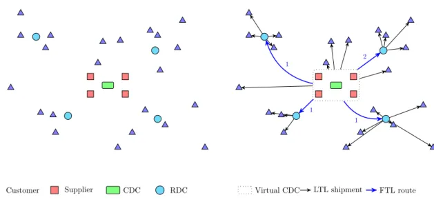
In this paper, we consider an economic sector in which the product distribution is free of charge for the customers. Thus, the collaborating companies want to maintain control of the distribution process and costs. In particular, they want to use only a few predefined distribution centers between their gates and the customers. This requirement is especially relevant if the product can be damaged by logistic operations. Figure 2 represents the multi-layered logistics network considered in our study. It is composed of four types of facilities:
• a set of suppliers: collaborating production centers which are the sources of all material flows,
• one consolidation and distribution center (CDC) which acts as the main collabo-rative warehouse at the suppliers gate,
• a set of regional distribution centers (RDC) which are end-of-line facilities in the collaborative network,
• a large set of customers who are the destinations of all product flows.
The capacity of the CDC and the RDCs is considered to be non-binding since there is only temporary storage.
Customer Supplier CDC RDC LTL shipment FTL route Supplier route
2.3 Supplier routes, FTL routes and LTL shipments
As shown in Figure 2, customer orders are consolidated and delivered to the customers through a sequence of three successive transportation segments called supplier routes, FTL routes and LTL shipments.
2.3.1 Supplier routes
Consolidation of shipments at the CDC requires local routes between the suppliers and the CDC. We call these routes supplier routes. Supplier routes pick up products from one or several suppliers and deliver them to the CDC. Since the number of collaborating companies is generally small, the potential number of supplier routes can be easily enu-merated. Moreover, supplier routes which are too long, raise scheduling incompatibilities or contain too many stops can be automatically discarded.
If the suppliers form a geographical cluster, the length of a supplier route is short (in our case between 5km to 80km). The cost of supplier routes is then mainly determined by fixed costs related to the driver, the vehicle and stopover costs at any intermediate stops (see e.g. [20] and [29]). In particular, we assume that it is independent of the number of units transported.
2.3.2 Full truckload routes
The use of FTL routes implicitly assumes that enough shipment have been consolidated, making it possible to fill a full truckload vehicle and send it to an RDC. FTL routes can start at the CDC or at a supplier and go directly to an RDC. Adding a pick up at an intermediate supplier or the CDC is also admitted, but this raises an additional stopover cost. In practice, many carriers will not accept routes with too much out-of-route distance [6], so that the set of potential FTL out-of-routes can be easily enumerated.
Each FTL route can be decomposed into a pickup leg, which is the part of the route where trucks are loaded (in the production area) and a long-haul leg between the last pickup point and an RDC.
The cost of the long-haul leg of an FTL route is assumed constant and known in advance. At least it can be approximated with good precision from previous experience of the companies.
The cost of a pickup leg is the sum of a cost proportional to the distance traveled and a constant stopover cost for each location visited after the starting point. Since all pickup legs can be easily enumerated, the mathematical model considers the set of all pickup legs, each one having a given known cost.
2.3.3 Less-than-truckload shipments
LTL shipments concern the distribution to final customers. These shipments are oper-ated by local transport companies. In practice, the distribution to final customers can be consolidated with goods supplied by other companies. The itineraries are designed
by the local operators and not controlled by the collaborating suppliers. This is why it is called LTL shipment.
We assume that all customer order are less-than-truckload quantities. In real life, there exist some exceptional orders which exceed one truckload. These orders are shipped directly from the supplier to the customer and are not considered here. There can also be some special operations that cannot be pooled with other orders. These orders are not considered by the present study.
We impose a single sourcing constraint: each customer is delivered from only one source, which can be a supplier, the CDC or an RDC. This prevents multiple deliveries of some customers on the same day and thus increases the quality of service. Note that from one day to another, one customer can be assigned to distinct distribution centers. This enables some flexibility by distributing the workload between the whole set of facilities.
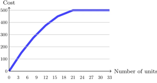
LTL shipments are delivered by vehicles which exact itinerary is unknown. As ex-plained in [21], the cost of an LTL shipment depends on the service provided by the local carrier and not on the usage of its resources. The cost increases non linearly with the number of units transported and incorporates discount rates, as represented in Figure 3.
0 100 200 300 400 500 0 3 6 9 12 15 18 21 24 27 30 33 Cost Number of units
Figure 3: Cost of an LTL shipment
Note that the cost of all LTL shipments are charged independently of each others, even if the customer orders are delivered by the same vehicle. We assume that this cost already integrate the possible handling costs at the RDC.
2.4 The collaborative load plan design problem (CLPDP)
The optimization problem at hand consists of assigning each customer order to one RDC, the CDC or a supplier and designing itineraries for all customer orders through the network. The objective function is to minimize the sum of transportation and handling costs. Since the CDC and the RDCs are used only as cross-docking facilities, there is no inventory cost.
Reduction of transportation costs can also be achieved through time aggregation. For example, if two suppliers send goods to a common customer on Mondays and Tuesdays respectively, there is no possible pooling of these orders. When a short-term storage is
possible, time consolidation is possible. This idea is exploited by [30] in a case where transportation costs depend on the time. The suppliers send one shipment containing all customer orders to a unique consolidation center, which stores the goods and sorts them by destination. This results in a non-linear optimization problem solved with a Lagrangean-based dual solution method.
We assume that the whole set of customer orders is partitioned into independent shipping dates. Volunteer postponement of the shipping in order to consolidate two successive orders is not authorized. However, the customers are driven to place regrouped orders. During the high season, the customer orders are frequent and larger. This reinforces the opportunity for shipping in FTL routes. During the low season, the customer orders are less frequent and generally concern very small shipments. The potential for FTL shipping is almost null, but large savings can be achieved if customers place regrouped orders.
Within each shipping date, the customers are delivered exactly once. Hence, shipping dates allow defining independent instances of the same optimization problem called Col-laborative Load Plan Design Problem (CLPDP). An MILP model for the (CLPDP)is presented in section 4.
3
Related research
Strategic collaboration between stakeholders of an existing supply chain has been studied by numerous authors. Among the multiple facets of collaborative distribution, the scope of the present paper is restricted to the optimization of logistics operations once all preliminary hurdles have been passed. In particular, our study concerns the optimization of the daily distribution operations in a predefined collaborative logistics network. We assume that strategic facility location decisions have met in a preliminary step and cannot be modified. The following subsections review some relevant research related to our work.
3.1 Horizontal cooperation among suppliers
The idea of consolidating customer orders has been existing for a long time, especially in the maritime and airline industry [2, 32]. As pointed out in [24] and [34], horizontal cooperation among carriers has been more studied than cooperation among shippers. See for example [22], [33] or [35].
Every large manufacturer with several production centers close enough to each others and customers scattered around a large geographical area faces the decision to consolidate its shipments. Such a company is described in [6], with a primary goal of saving sales reps time through improvement of the information system and a secondary goal of saving some transportation cost.
Most research about horizontal collaboration focuses on the strategic level, with a main concern of designing the supply chain network. In these model, typical binary decisions concern the location of pooled facilities. Continuous or integer decisions
con-cern the flow of material between facilities. Economic models often come along with the reduction of greenhouse gas emissions and the use of inter-modal transportation. For example, the effect of pooling the supply chains of two major French retailer chains, with the aim of reducing CO2 emissions from freight transport is explored in [28]. This study
yields a relative reduction of CO2 emissions of 14% exclusively with road transport and
52% when combining of road and rail. A collaborative many-to-many collaborative hub network in the Netherlands is studied in [16]. The shipments through the hub network uses inland navigation by barges. One common point with our study is that customer’s demand may be split into a fraction using the hub network (or CDC) and another frac-tion which is shipped directly by companies. A reducfrac-tion of average logistics costs of 14% is reported for freight using the hub network.
Two applications in the area of automotive industry in Europe are presented in [24]. The first application concerns distribution from 7 automotive companies of Romania to a set of destinations all over Europe. The authors propose two scenarios with inter-modal transportation: train + direct delivery by truck or train + transport bundling. The cost reduction is by 14%. The second application concerns the distribution from suppliers in Eastern Spain to Saxony. LTL demands are first consolidated before being carried to Germany. This yields a cost reduction by 15% and a fuel consumption and CO2 emissions reduction by 17%.
Freight consolidation between small companies which generally ship less than truck-load quantities is also studied in [34]. They consider stochastic arrival of suppliers orders and create ad hoc freight consolidation on each route and each time period. They show that coalition outperforms the myopic approach especially when the arrival rate is low. They observe that “for small shippers to obtain savings, the origin and the destination of the shipment must be in relatively close proximity.”
In factory gate pricing (FGP) the products are collected by the retailer at the gates of the suppliers. Seven FGP scenarios are studied in [5], in the area of slow moving dry grocery goods. The use of a consolidation hub between suppliers and synchronization efforts can save up to 26% of the logistics costs. As further research, the authors indicate the possibility of bypassing the retailers distribution centers, optimizing the location of the consolidation hub and dealing with seasonal variations.
3.2 Service network design
The collaborative load plan design problem is related to service network design [8]. One key issue in this domain is to plan the service of a fleet of vehicles and the routing of orders from origins to end-of-line terminals through transshipment centers. This problem often uses several modes of transport. This problem is also called load plan design and has been receiving a lot of attention from the OR community in recent years [3, 9, 12, 13]. This research aims at minimizing LTL freight transportation carrier costs. It mostly concerns transport on very large territories where one trip from a transshipment center to another may take more than one day and the management of assets as well as delay considerations are major issues. The construction of routes with several pickup points is not considered in these applications.
Lindsey et al. [25] consider the problem of transporting products from suppliers to distribution centers using LTL and FTL services in the retail industry. To our knowledge, this work is the only one to consider the design of subcontracted FTL routes with multiple shipment origins and destinations. The problem uses a path based formulation. Restrictions of this problem are solved sequentially and find solutions to large instances within 4h of run-time.
Krajewska and Kopfer [21] define the integrated transportation planning problem (ITPP) as the problem of constructing a load fulfillment plan, assuming a fixed lim-ited size of the owned fleet and predefined types of LTL external carriers. Splitting of customer orders is not allowed.
3.3 Modeling the transportation costs
One of the main incentives for horizontal collaboration is the cost structure charged by the carriers for LTL shipments. As detailed in [36], this cost depends on both tangible and intangible factors. Examples of intangible factors are the degree of competition on the local markets, the desirability of the shipment or the negotiation power of the shipper. In can be also influenced by inevitable empty truck repositioning [14].
One classical approach is to consider a cost structure with incremental discounts, leading to a concave function which can be approximated by a piecewise linear function, as shown in Figure 3. This approximation is practical for optimization purposes but sometimes not realistic. The Modified All-Unit Discount (MAUD) cost structure is based on weight intervals on which decreasing prices are incurred [27]. For example, shipments with less than 30kg are charged $ 30/kg and shipments with more than 45 kg are charged $ 20 / kg. This leads to a non-continuous piecewise affine cost curve with breakpoints. In order to avoid breakpoints and keep the price curve monotonously non-decreasing, the whole interval [30,45] is charged as 45kg for $ 20/kg. Example of MAUD cost structures can be found in [17] or [36] in the context of LTL shipments and in [19] in the context of air transportation. [23] present a compound cost function merging the best use of each category of transport: parcel, LTL or FTL depending on the shipment weight.
3.4 Related topics not included in the present paper
Before solving logistic issues, many management and technological issues must be fixed. Among management aspects, the identification and selection of potential partners [1, 10] and the building of trust within the coalition [16, 18, 24] are crucial success factors. Run-ning a collaborative logistics systems also requires sharing a part of the commercial and logistic information. This often implies using collaborative information and communi-cation technologies [7, 10, 26] which enable building consolidated load plans without disclosing sensitive strategic or commercial information.
Optimization of collaborative transportation practices aims at minimizing the dis-tribution cost or maximizing the profit of the whole coalition. Thus, the cost allocation and the sharing of benefits is a crucial issue generally solved with game theory tools.
The objective is to find a stable coalition, i.e. a business model such that every player individually benefits from the strategic alliance. For each player, there may exist a mini-mum percentage of savings necessary to join the coalition. The influence of this minimal value on the global benefits is measured in [4]. Various profit allocation mechanisms are discussed in [11] and [31].
3.5 Position of the present study
Our study concerns the operational level decisions in the context of shipper collabora-tion. We assume that strategic decisions such as facility location have been already met and we concentrate on the daily allocation of customer to distribution centers and the optimization of material flows in the distribution network.
In our study, the main focus is set on cost minimization. The quality of service to customers and the reduction of CO2 emissions are considered as collateral benefits of
a proper use of the distribution network, but these elements are not integrated in our mathematical model. The main difficult in our study comes from the combination of FTL and LTL shipments in a multi-layered network. Since we assume that a customer order is delivered at once, the cost of an LTL shipment represents only one point on the concave cost function represented in Figure 3. Thus, the delivery cost from one distribution center to a customer is a constant value.
One original feature of our model is that the CDC is seen as a means to facilitate the implementation of the horizontal collaboration, but the transit of goods by the CDC is not mandatory. Customer orders can be shipped directly from suppliers to RDCs or to customers without being processed at the CDC. This avoids break bulk cost. Our study potentially concerns any type of goods provided they can be carried in common vehicles. We also assume that all customer orders can be expressed with a single metric (e.g. a number of pallets or boxes) If several types of containers exist, or if bulk is transported, conversion factors are used to express all quantities with this reference metric.
4
Modeling of the (CLPDP)
We consider a set S of suppliers and a set I of customers. The quantity ordered by customer i ∈ I to a supplier s ∈ S is denoted by qis. We also write qi =Ps∈Sqis. Let J
be the set of distribution centers, which includes the CDC (index 0) and the set J? ⊂ J of RDCs. With each j ∈ J?, we associate an FTL route operated by a homogeneous fleet Kj of vehicles with capacity Qk. The complete set of vehicles on FTL routes is
denoted by K =S
j∈J?Kj. We denote by Λ the set of all possible pickup legs. Subsets
Λs⊂ Λ and Λ0 ⊂ Λ denote the pickup legs that visit supplier s ∈ S and the pickup legs
that visit the CDC, respectively. Finally, we denote as Γ the set of all possible supplier routes. A supplier route γ ∈ Gamma is operated by a homogeneous fleet of vehicles with capacity Qγ.
The transportation and handling costs as defined as follows. cdist
ij is the distribution
customer orders cannot be split in several LTL shipments, so that the cost cdist ij is a
constant value. The cost of an FTL route includes the cost cftl
j of the long-haul leg and
the cost cpl
λ of the pickup leg λ ∈ Λ. The cost of a supplier route γ ∈ Γ is denoted by
csr
γ . The unitary handling cost at the CDC is denoted by h. Handling costs must be
payed for all products that are unloaded at the CDC.
The mixed integer linear program has four sets of binary or integer decision variables. First, for all i ∈ I and j ∈ J , xij= 1 if customer i is served by the distribution center
or supplier j ∈ J ∪ S, and 0 otherwise. For all k ∈ K, lk = 1 if FTL vehicle k is used,
0 otherwise. In addition, vkλ = 1 if FTL vehicle k ∈ K takes pickup leg λ ∈ Λ, and
0 otherwise. The integer variable nγ indicates the number of vehicles on supplier route
γ ∈ Γ. Three sets of continuous positive variables model the material flow through the network. The variable wkλis represents the number of units shipped from supplier s ∈ S to customer i ∈ I and carried by vehicle k ∈ K on pickup leg λ ∈ Λ. For each supplier s ∈ S, the variable usγ ∈ [0, Qγ] is the number of units loaded at supplier s on supplier
route γ ∈ Γ. The variable u0sk ∈ [0, Qk] is the quantity supplied by s that is loaded onto an FTL vehicle k ∈ K at s and unloaded at the CDC (in this case, the FTL route has some residual capacity which is used as a supplier route).
The (CLPDP) problem can be modeled as follows:
min z =X γ∈Γ csr γ nγ+ X λ∈Λ X k∈K cpl λ vkλ+ X j∈J? X k∈Kj cftl j lk+ X i∈I X j∈J ∪S cdist ij xij+h X s∈S (X k∈K u0sk+X γ∈Γ usγ) (1)
s.t. X j∈J ∪S xij = 1 ∀i ∈ I (2) X k∈Kj X λ∈Λ wiskλ= qisxij ∀s ∈ S, ∀i ∈ I, ∀j ∈ J? (3) X s∈S X i∈I X λ∈Λ wiskλ≤ Qklk ∀k ∈ K (4) X λ∈Λ vkλ= lk ∀k ∈ K (5) wiskλ ≤ vkλqis ∀k ∈ K, ∀i ∈ I, ∀s ∈ S, ∀λ ∈ Λs∪ Λ0 (6) u0sk+X i∈I wkλis ≤ Qkvkλ ∀s ∈ S, ∀k ∈ K, ∀λ ∈ Λs∩ Λ0 (7) X γ∈Γs usγ + X k∈K u0sk = X i∈I qisxi0+ X λ∈Λ0\Λs X k∈K X i∈I wkλis ∀s ∈ S (8) X s∈S usγ ≤ Qγnγ γ ∈ Γ (9) xij ∈ {0, 1} ∀i ∈ I, ∀j ∈ J ∪ S (10) lk∈ {0, 1} ∀k ∈ K (11) vkλ∈ {0, 1} ∀k ∈ K, ∀λ ∈ Λ (12) nγ∈ N ∀γ ∈ Γ (13) wiskλ ∈ [0, qis] ∀i ∈ I, ∀λ ∈ Λ (14) u0sk ∈ [0, Qk] ∀s ∈ S, ∀k ∈ K (15) usγ ∈ [0, Qγ] ∀s ∈ S, ∀γ ∈ Γ. (16)
The objective function (1) contains five components corresponding to the supplier routes, the base cost of FTL route, the pickup legs, the LTL shipment and the cross-docking at the CDC. Constraints (2) state that each customer must be delivered from one unique distribution center or supplier. Conservation flow constraints (3) state that the whole quantity of goods arriving at an RDC is shipped to the customers served by this RDC. Constraints (4) are capacity constraints for FTL vehicles. Constraints (5) state that an utilized pickup leg (lk = 1) should be associated with a vehicle k ∈ K.
Constraints (6) state that if vehicle k ∈ K does not visit a pickup leg λ ∈ Λ, then wiskλ must be 0. Constraints (7) state that some residual capacity on a pickup leg going from a supplier s to the CDC may be used to transport goods to the CDC. Constraints (8) model flow conservation of supplier s products at the CDC: the incoming flow is the quantity transported by supplier routes and on the residual capacity of FTL vehicles. The outgoing flow corresponds to shipments from the CDC and loading in FTL vehicles.
Constraints (9) state that the flow on a supplier route γ is limited by the number of vehicles on this route and their capacities. The following constraints define the nature and the domain definition of all variables.
5
Decomposition method
The main idea of our decomposition approach is to sequentially set the value of all deci-sions variables. This leads to three steps, each of them being modeled by a mixed integer linear problem. These MILPs are much easier to solve than the original (CLPDP), so that it is hoped that the decomposition yields good feasible solutions within an accept-able calculation time.
In the first step, we solve a subproblem called (SP1) which allocates customers to distribution centers (variables xij) and determines the number of vehicles on each FTL
route (variables lk). Then, one subproblem (SP2) is solved separately for each RDC. It
determines the pickup leg of each FTL vehicle (variables vkλ) and dispatches customer
orders in these vehicles (variables wkλis ). Finally, subproblem (SP3) designs supplier routes to consolidate orders at the CDC (variables nγ and u0sk). The three subproblems
are described in sections 5.1, 5.2 and 5.3.
5.1 Subproblem (SP1): customer allocation and design of FTL routes
The Figure 4 represents the input (left part) and the output (righ part) of subproblem (SP1). In this step, all suppliers and the CDC are aggregated into a virtual CDC. The main consequence is that FTL routes have no pickup leg anymore, so that there is only one possible FTL route between the virtual CDC and each RDC. Moreover, the cost of the FTL route to j ∈ J∗ is limited to the cost cftl
j of the long-haul leg.
In the output of subproblem (SP1), customers are assigned either to one RDC or to the virtual CDC and the number of FTL vehicles required on each FTL route is determined.
1
1
2
1
Customer Supplier CDC RDC Virtual CDC LTL shipment FTL route
Figure 4: Subproblem (SP1) input and output
5.1.1 Modeling of subproblem (SP1)
We denote by ˜J the set of distribution centers where the CDC has been replaced by the virtual CDC. For each customer i ∈ I, the shipment cost ˜cdist
i0 from the virtual CDC
is redefined as follows: if customer i has a demand for only one supplier s ∈ S then ˜
cdist
i0 = cdistis , otherwise, ˜cdisti0 = cdisti0 . For each customer i ∈ I and each j ∈ ˜J , we use
the boolean variable ˜xij, which is equal to 1 if customer i is served by j, 0 otherwise.
For all j ∈ J?, the positive integer variable yj denotes the number of FTL trucks that
have to be sent to j. (SP1) can then be modeled as follows:
min z1 = X j∈J? cftl j yj + X i∈I X j∈ ˜J cdist ij x˜ij (17) s.t. X j∈ ˜J ˜ xij = 1 ∀i ∈ I (18) X i∈I qix˜ij ≤ Qyj ∀j ∈ J? (19) yj ∈ N, ∀j ∈ J? (20) ˜ xij ∈ {0, 1} ∀i ∈ I, j ∈ ˜J . (21)
This optimization problem can be modeled as a capacitated facility location problem where each FTL route can be seen as a capacity to serve customers from an RDC. The objective function (17) minimizes the cost of FTL routes and LTL shipments. Con-straints (18) state that each customer should be delivered by one facility. ConCon-straints
(19) computes the number of FTL vehicles needed to transport the orders assigned to each RDC.
5.1.2 Output
The output of (SP1) can be used as follows to fix the variables of model (CLPDP). For each i ∈ I and each j ∈ J?, we set xij = ˜xij. For a customer i assigned to the
virtual CDC, if customer i has a demand for only one supplier s ∈ S, then the orders are all shipped from s (xis = ˜xi0= 1). If customer i orders to at least two suppliers, it
is assigned to the CDC (xi0= ˜xi0= 1).
For each j ∈ J?, we create a set ˜Kj ⊆ Kj of vehicles, with | ˜Kj| = yj. The decision
variable lk of the (CLPDP) is set to 1 for all k ∈ ˜Kj and to 0 otherwise.
5.2 Subproblem (SP2): design of FTL routes and load planning
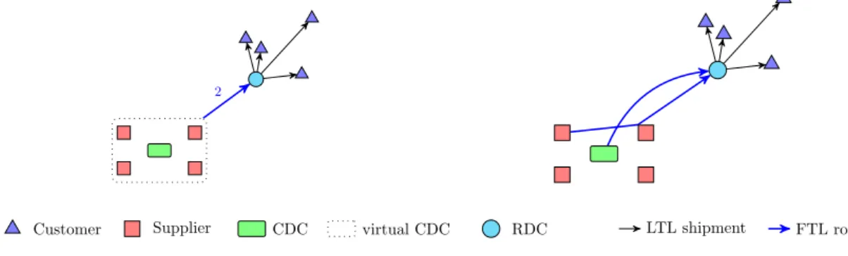
In the second step, one distinct instance of subproblem (SP2) is solved for each RDC. Figure 5 illustrates the input and output of subproblem (SP2) corresponding to the north east RDC denoted j. The problem consists of (i) determining the pickup leg that should be assigned to each of the | ˜Kj| FTL vehicles that serve j; (ii) for each customer i
that has a demand qis to a supplier s, the portion of this demand carried by each vehicle.
2
Customer Supplier CDC virtual CDC RDC LTL shipment FTL route
Figure 5: Subproblem (SP2) input and output for a given RDC
5.2.1 Subproblem (SP2) notation and assumptions
For a given j ∈ J?, the solution of subproblem (SP1) yields a set ˜Kj of FTL vehicles
that serve j. We also define the set Ij of customers assigned to j.
(SP2) determines the value of binary variables vkλ which are equal to 1 if truck
k ∈ ˜Kj starts with pickup part λ ∈ Λ, and continuous variables wkλis ∈ [0, qis], which
represents the number of units from the order of customer i to supplier s that are transported in vehicle k ∈ ˜Kj on pickup part λ ∈ Λ.
In subproblem (SP2), it is assumed that the residual capacity on a pickup leg from a supplier s to the CDC cannot be used to replace supplier routes (i.e. variables u0sk are ignored). It is also assumed that all supplier routes are direct trips from suppliers to the
CDC. The cost θs of each unit carried on the supplier route between supplier s ∈ S and the CDC is approximated to θs= h + csr γ Qγ. 5.2.2 Modeling of subproblem (SP2)
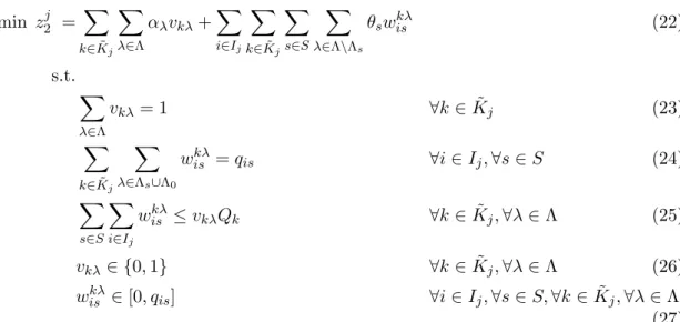
For a given j ∈ J?, we model the subproblem (SP2)j as follows:
min z2j = X k∈ ˜Kj X λ∈Λ αλvkλ+ X i∈Ij X k∈ ˜Kj X s∈S X λ∈Λ\Λs θswiskλ (22) s.t. X λ∈Λ vkλ= 1 ∀k ∈ ˜Kj (23) X k∈ ˜Kj X λ∈Λs∪Λ0 wkλis = qis ∀i ∈ Ij, ∀s ∈ S (24) X s∈S X i∈Ij wiskλ≤ vkλQk ∀k ∈ ˜Kj, ∀λ ∈ Λ (25) vkλ ∈ {0, 1} ∀k ∈ ˜Kj, ∀λ ∈ Λ (26) wiskλ∈ [0, qis] ∀i ∈ Ij, ∀s ∈ S, ∀k ∈ ˜Kj, ∀λ ∈ Λ (27)
The first sum in the objective function (22) represents the cost of the selected pickup legs. The second sum is an estimation of the supplier routes cost for the remaining goods. Constraints (23) state that one unique pickup leg is assigned to each vehicle. Constraints (24) ensure the satisfaction of customers demand, stating that an order from supplier s can be transported in a vehicle that either visits s or the CDC. Constraints (25) state that the sum all of demands on a pickup leg λ ∈ Λ should not exceed the vehicle capacity Qk.
5.3 Subproblem (SP3): selection of supplier routes
Supplier routes are used to transport the goods that must be pickup up at suppliers and delivered to the CDC. Then, these goods can be shipped directly to customers or loaded onto FTL vehicles. Once customer orders have been assigned to distribution centers and all FTL vehicle itineraries are set, (SP3) selects the supplier routes and the number of vehicles on each supplier route.
We recall that when the pickup leg of an FTL route visits a supplier s before visiting the CDC, the residual capacity of the FTL vehicles can be used to ship goods between s and the CDC at no additional cost. Note that an explicit assignment of every customer order to the vehicles on supplier routes is not required here: the model ensures that the capacity on supplier routes is sufficient to supply the CDC.
Customer Supplier CDC RDC LTL shipment FTL route supplier route
Figure 6: Subproblem (SP3) input and output
5.3.1 Subproblem (SP3): input and notation
We denote by qs0 the total load that has to be transported from a supplier s ∈ S to the CDC. According to the results of (SP1) and (SP2), qs0 can be calculated as follows:
q0s=X i∈S qisxi0+ X i∈I X k∈K X λ∈Λ0\Λs wiskλ.
The first sum represents the orders that are shipped from the CDC and the second sum represents the number of units loaded onto FTL vehicles at the CDC.
The set of vehicles that use the pickup leg λs0 ∈ Λs∩ Λ0 from a supplier s ∈ S to
the CDC (e.g. such that vkλs0 = 1) is denoted by K
0
s. The residual capacity on a vehicle
k ∈ Ks0 is denoted by Qks.
For each supplier route γ ∈ Γ, (SP3) determines the value of variable nγ ∈ N
repre-senting the number of vehicles on route γ. For each supplier s ∈ S, it also determines the value of the continuous variables usγ, for all γ ∈ Γ and u0sk, for all k ∈ Ks0. These
variables represent the load from supplier s on supplier route γ and on the residual capacity of FTL vehicle k pickup leg, respectively.
5.3.2 Modeling of subproblem (SP3) min z3 = X γ∈Γ cγnγ (28) s.t. X γ∈Γs usγ+ X k∈K0 s u0sk ≥ qs0 ∀s ∈ S (29) X s∈S usγ ≤ Qγ× nγ ∀γ ∈ Γ (30) nγ ∈ N ∀γ ∈ Γ (31) usγ ∈ [0, Qγ] ∀s ∈ S, ∀γ ∈ Γs (32) u0sk ∈ [0, Qk s] ∀s ∈ S, ∀k ∈ Ks0. (33)
The objective function (28) minimizes the cost of supplier routes. Constraints (29) enforce the total load of each supplier to be transported to the CDC, either by using the residual capacity on FTL pickup legs or through supplier routes. Constraints (30) connects the load on each supplier route to the number of vehicles needed on this route according to the supplier vehicles capacity Qγ.
6
Experiments and case study
In this section, we present numerical experiments on a real-life case study. All models have been coded in Java using the Concert Technology framework of CPLEX 12.6. Tests were run on a PC Intel Core i7-4600U processor 2.1 Ghz with 16 Gb of memory under the System Windows 8.1. For all models solved in this section, the best parameters of CPLEX were determined with the CPLEX tuning tool.
According to an agreement with the suppliers in this study, no cost or indication on savings provided by collaboration can be presented in this paper. We focus on the assessment of the decomposition approach, comparing runtime and gap with the lower bound provided by the solving of the (CLPDP) model.
6.1 The distribution network
The distribution network includes 7 suppliers, 1 CDC, 6 RDCs and 5128 customers. The suppliers form a geographical cluster in Western France: the maximal distance between two facilities is only 60 km. Customers are mainly specialized stores (65%), supermarkets or retail stores (26%), but also resellers, local authorities, schools, etc. They are spread over the whole territory, with an average distance of 380 km to the suppliers. The average quantity per shipment is only 2.6 units. We observe that a few hundreds major regular customers generally order to several suppliers among the 7 collaborating companies. Besides, a large number of customers order very small quantities and many occasional customers order only once or a few times a year.
The set Λ of pickup legs of FTL routes can either include the CDC (1 possibility), one supplier only (|S| possibilities), or one supplier plus another supplier or the CDC (|S| × ((|S| − 1) + 1) possibilities). So, we have |Λ| = 1 + 7 + 7 × 7 = 57 pickup legs. This results in 57 × 6 = 342 feasible FTL routes. The set Γ of supplier routes includes direct trips from a supplier to the CDC (7 possibilities) or trips with one stopover at another supplier before delivering the CDC (|S| × (|S| − 1 possibilities). So, we have |Γ| = 7 + 7 × 6 = 49 supplier routes.
6.2 Data collection
We dispose of an exhaustive recording of one complete year of activity representing 74039 shipments. The number of weekly deliveries is 3 during the high season, 2 during the mid-season and 1 during the low season. This results in 121 shipping dates, and then in 121 instances. The number of units considered in an instance varies between 6 and 6345.
We empirically observed that the cost of LTL shipments from the production area to all customers follows a MAUD cost structure. Unfortunately, since each shipment concerns small discrete quantities, identifying breakpoints and capturing the parameters of the cost curve was impossible in practice due to the lack of data. Moreover, the cost of LTL shipments from RDCs to customers is not known with much precision. In order to generate realistic LTL shipment costs, we aggregated customers from each of the 95 French departments and established a list of 1134 distinct known costs. Then, we followed the approach of [5] and [36] and estimated the costs by means of a regression model. The LTL cost could be expressed with good accuracy as a non-linear function of the number of units and the distance between the origin and the destination.
6.3 Solving model (CLPDP)
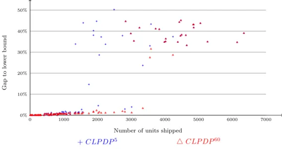
All 121 (CLPDP) instances were solved with a computing time of 5 minutes and 1 hour respectively. The shorter computation time is considered as acceptable for a daily use of the model and simulations of various scenarios. The results related to each computational time are denoted as CLP DP5and CLP DP60respectively. They are presented in Figure
7. Each point in this figure represents the performance of CPLEX on one instance. The horizontal axis represents the total customer demand expressed in number of logistic units. The vertical axis represents the relative gap between the lower bound Zlb and the
upper bound Z provided by the solver. It is computed as (Z − Zlb)/Zlb× 100.
It is clear that only some small instances can be solved to optimality within an acceptable time. When the solving time is increased, the results found on large instances remain really far from the lower bound.
As far as CLP DP5 is concerned, the optimality gap suddenly becomes very large when the number of units exceeds 1300. It is 30.5% on average for instances with more than 1300 units.
Only instance with up to 400 units could be solved to optimality by CLP DP60. The optimality gap increases quickly when the number of units exceeds 2800. It is 34.3% on
0 0% 1000 2000 3000 4000 5000 6000 7000 10% 20% 30% 40% 50%
Number of units shipped
Gap to lo w er b ound + CLP DP5 4 CLP DP60
Figure 7: Results of CLP DP5 and CLP DP60
average on instances with more than 2800 units.
6.4 Results of the decomposition approach
The decomposition into subproblems (SP1), (SP2) and (SP3) was solved with an al-lowed computation time of 5 minutes spread over all models, and then with no time limit. Theses results are denoted as SP5 and SP∗ respectively.
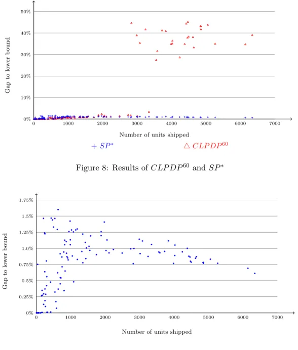
Figure 8 compares the results of CLP DP60 and SP∗. For SP∗, we calculate the relative gap with the lower bound given by CLP DP60. On small instances, the opti-mality gaps of SP∗ and CLP DP60 are comparable. On larger instances, a remarkable
fact is that the size of the instances does not seem to influence the performance of the decomposition approach: very good solutions can be reached even on large instances. Another remark is that the lower bound found by CPLEX while solving the (CLPDP) is actually very close to a feasible solution.
Figure 9 shows the gap between the upper bound provided for SP5 and the lower bound given by CLP DP60. In fact, results found by SP5 and SP∗ are almost identical: they have the same minimal gap (0.0%), average gap (0.75%) and maximal gap (1.6%). Table 1 shows how computation times is spread over the solving of subproblems (SP1), (SP2) and (SP3) in scenarios SP5 and SP∗. The objective of this table is to assess the practical difficulty of each subproblem. Clearly, subproblem (SP2) is the most difficult one with an average required computation time running time of 385.7 seconds and a maximal computation time of 3524 seconds for SP∗. Given that the numerical results of scenarios SP5 and SP∗are almost identical, we observe that optimal solutions of subproblem (SP2) can be found quickly but optimality is hard to prove.
0 0% 1000 2000 3000 4000 5000 6000 7000 10% 20% 30% 40% 50%
Number of units shipped
Gap to lo w er b ound 4 CLP DP60 + SP∗
Figure 8: Results of CLP DP60 and SP∗
0 0% 1000 2000 3000 4000 5000 6000 7000 0.25% 0.5% 0.75% 1.0% 1.25% 1.5% 1.75%
Number of units shipped
Gap to lo w er b ound Figure 9: Results of SP5
Table 1: Computation time in each subproblem (in seconds)
SP∗ SP5
Avg Time Max Time Avg Time Max Time
(SP1) 0.3 4 0.3 3
(SP2) 385.7 3524 53.0 300
6.5 Detailed results
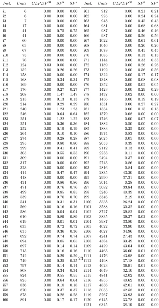
Table 2 details the results found by each algorithm for each instance. Columns la-beled Inst and U nits stand for the name of instance and the number of shipped units. Columns labeled CLP DP60, SP5 and SP∗ represent the relative gap between scenarios CLP DP60, SP5 and SP∗. The relative gaps are calculated between the solution value
Z of each scenario and the best solution value Zbest among the three scenarios. It is
computed as (Z − Zbest)/Zbest× 100. CLP DP60 finds 80 best solutions, SP∗ finds 55
best solutions, out of them 49 are also found by SP5. On 15 instances CLP DP60, SP5
and SP∗ find solutions with identical costs. Table 2 indicates identical value for scenar-ios SP5 and SP∗ on all but 3 instances. In reality, 5 more results slightly differ between both scenario, but with a gap less than 0.01%. We can notice that exactly solving the original model never outperforms the decomposition approach by more than 1.5%. On the contrary, for all large instances, the decomposition approach clearly outperforms scenario CLP DP60.
7
Conclusion
In this paper, we considered the routing of customer orders in a collaborative distribu-tion network for a set of neighbor suppliers who want to reduce their distribudistribu-tion cost. We defined the Collaborative Load Plan Design Problem (CLPDP) which concerns the operational level decisions on each shipping date. It consists of assigning customers to end-of-line distribution centers, determining the material flow along three successive transportation segments: supplier routes, FTL routes and LTL shipments. We intro-duced a mixed integer linear programming formulation for this problem and proposed to decompose it into three subproblems which are sequentially solved. The experiments on a full year of distribution orders showed that model (CLPDP) cannot be solved efficiently by a state-of-the-art solver. On the contrary, the decomposition provides near optimal solutions within a few minutes.
Adding valid inequalities to the (CLPDP) model or finding a stronger formulation would probably help solving it more efficiently, but the lower bound found by CPLEX is already very good. In future research, we intend to extend the present problem by considering several additional assumptions. In many real-life cases, several types of con-tainers are used to ship the products. Customers are located in geographical areas which are given priority levels. These two new rules complicate the load plan. We considered that the long-haul leg of FTL routes visit only one RDC and that its cost is constant. In practice, there can exist long-haul legs with two RDCs and also intermediate costs for a few partial loads. Finally, we assumed an already existing network with imposed RDC locations. We also assumed that the allocation of customer to RDCs could be revised everyday. In many real cases, a preliminary strategic problem is to select the RDCs among a large set of potential candidate locations. For practical reasons, it is safer to set customer-RDC allocation at least for one season. Hence, the optimization of collab-orative distribution networks raises many additional strategic, tactical and operational
Table 2: Relative performance of scenarios CLP DP60, SP∗ and SP5 (gaps in % to the lower bound returned by CLP DP60)
Inst. Units CLP DP60 SP5 SP∗ i1 6 0.00 0.00 0.00 i2 6 0.00 0.00 0.00 i3 7 0.00 0.00 0.00 i4 17 0.00 0.00 0.00 i5 41 0.00 0.75 0.75 i6 41 0.00 0.00 0.00 i7 60 0.00 0.00 0.00 i8 63 0.00 0.00 0.00 i9 67 0.00 0.00 0.00 i10 73 0.00 0.00 0.00 i11 76 0.00 0.00 0.00 i12 124 0.03 0.00 0.00 i13 152 0.00 0.26 0.26 i14 158 0.00 0.00 0.00 i15 168 0.00 0.34 0.34 i16 169 0.00 0.00 0.00 i17 176 0.00 0.27 0.27 i18 208 0.00 1.47 1.47 i19 213 0.00 0.13 0.13 i20 214 0.00 0.29 0.29 i21 240 0.00 1.23 1.23 i22 246 0.00 0.64 0.64 i23 251 0.00 1.22 1.22 i24 251 0.00 0.36 0.36 i25 252 0.00 0.19 0.19 i26 264 0.00 0.10 0.10 i27 274 0.00 0.28 0.28 i28 295 0.00 0.80 0.80 i29 299 0.00 0.41 0.41 i30 305 0.00 0.55 0.55 i31 309 0.00 0.00 0.00 i32 317 0.00 0.00 0.00 i33 323 0.00 0.00 0.00 i34 414 0.00 0.47 0.47 i35 418 0.00 0.00 0.00 i36 431 0.00 0.86 0.86 i37 471 0.00 0.76 0.76 i38 499 0.00 0.85 0.85 i39 539 0.00 0.70 0.70 i40 541 0.00 0.31 0.31 i41 569 0.00 0.16 0.16 i42 586 0.00 0.04 0.04 i43 610 0.00 0.89 0.89 i44 619 0.00 0.01 0.01 i45 633 0.00 0.72 0.72 i46 635 0.00 0.36 0.36 i47 692 0.00 0.74 0.74 i48 694 0.00 0.05 0.05 i49 697 0.00 0.14 0.14 i50 715 0.00 0.16 0.16 i51 742 0.00 0.29 0.29 i52 749 0.00 0.25 0.25 i53 797 0.00 0.14 0.14 i54 808 0.00 0.34 0.34 i55 824 0.00 0.55 0.55 i56 825 0.00 0.64 0.64 i57 836 0.00 0.18 0.18 i58 870 0.00 0.37 0.37 Inst. Units CLP DP60 SP5 SP∗ i61 912 0.00 0.21 0.21 i62 925 0.00 0.24 0.24 i63 948 0.00 0.45 0.45 i64 981 0.00 0.68 0.68 i65 987 0.00 0.46 0.46 i66 987 0.00 0.56 0.56 i67 1022 0.00 0.61 0.61 i68 1046 0.00 0.26 0.26 i69 1078 0.00 0.45 0.45 i70 1085 0.00 0.13 0.13 i71 1144 0.00 0.33 0.33 i72 1189 0.00 0.26 0.26 i73 1192 0.00 0.56 0.56 i74 1322 0.00 0.17 0.17 i75 1348 0.00 0.08 0.08 i76 1352 0.00 0.05 0.05 i77 1423 0.00 0.29 0.29 i78 1437 0.02 0.00 0.00 i79 1456 0.00 0.19 0.19 i80 1531 0.00 0.27 0.27 i81 1554 0.00 0.15 0.15 i82 1579 0.08 0.00 0.00 i83 1746 0.00 0.07 0.07 i84 1882 0.50 0.00 0.00 i85 1883 0.25 0.00 0.00 i86 1974 0.83 0.00 0.00 i87 2025 0.05 0.00 0.00 i88 2053 0.39 0.00 0.00 i89 2112 0.13 0.00 0.00 i90 2238 0.11 0.00 0.00 i91 2494 0.37 0.00 0.00 i92 2743 0.86 0.00 0.00 i93 2816 0.84 0.00 0.00 i94 2835 43.20 0.00 0.00 i95 2990 37.31 0.00 0.00 i96 3014 0.28 0.00 0.00 i97 3082 33.84 0.00 0.00 i98 3246 40.39 0.00 0.00 i99 3346 2.19 0.00 0.00 i100 3558 26.24 0.00 0.00 i101 3588 30.32 0.00 0.00 i102 3727 39.82 0.00 0.00 i103 3835 39.37 0.02 0.00 i104 3987 33.80 0.00 0.00 i105 4022 33.90 0.00 0.00 i106 4027 34.96 0.00 0.00 i107 4241 27.43 0.00 0.00 i108 4384 33.49 0.00 0.00 i109 4429 43.04 0.00 0.00 i110 4463 36.60 0.01 0.00 i111 4476 43.98 0.00 0.00 i112 4498 37.18 0.00 0.00 i113 4623 36.91 0.01 0.00 i114 4649 32.10 0.00 0.00 i115 4841 42.02 0.00 0.00 i116 4855 40.62 0.00 0.00 i117 4856 42.01 0.00 0.00 i118 5055 42.58 0.00 0.00 23
problem which still deserve much research effort.
Acknowledgements: This research was partially funded by the FUI (Fonds unique interminist´eriel) and labeled by the competitive clusters Vegepolys and Nov@log. This support is gratefully acknowledged.
References
[1] Adenso-D´ıaz, B., Lozano, S., Moreno, P.: Analysis of the synergies of merging multi-company transportation needs. Transportmetrica A: Transport Science 10(6), 533–547 (2014)
[2] ´Alvarez-SanJaime, O., Cantos-S´anchez, P., Moner-Colonques, R., Sempere-Monerris, J.J.: Competition and horizontal integration in maritime freight trans-port. Transportation Research Part E: Logistics and Transportation Review 51, 67–81 (2013)
[3] Andersen, J., Christiansen, M., Crainic, T.G., Grønhaug, R.: Branch and price for service network design with asset management constraints. Transportation Science 45(1), 33–49 (2011)
[4] Audy, J.F., D’Amours, S., Rousseau, L.M.: Cost allocation in the establishment of a collaborative transportation agreement - an application in the furniture industry. Journal of the Operational Research Society 62(10), 960–970 (2011)
[5] le Blanc, H., F., C., Fleuren, H., de Koster, M.: Factory gate pricing: An analysis of the dutch retail distribution. European Journal of Operational Research 174(3), 1950–1967 (2006)
[6] Brown, G., Ronen, D.: Consolidation of customer orders into truckloads at a large manufacturer. Journal of the Operational Research Society 48(8), 779–785 (1997)
[7] Buijs, P., (“Hans”) Wortmann, J.: Joint operational decision-making in collabo-rative transportation networks: the role of it. Supply Chain Management: An International Journal 19(2), 200–210 (2014)
[8] Crainic, T.G.: Service network design in freight transportation. European Journal of Operational Research 122(2), 272–288 (2000)
[9] Crainic, T.G., Hewitt, M., Toulouse, M., Vu, D.M.: Service network design with resource constraints. Transportation Science (2014). DOI 10.1287/trsc.2014.0525
[10] Cruijssen, F., Cools, M., Dullaert, W.: Horizontal cooperation in logistics: Oppor-tunities and impediments. Transportation Research part E 43(2), 129–142 (2007)
[11] Dai, B., Chen, H.: Profit allocation mechanisms for carrier collaboration in pickup and delivery service. Computers and Industrial Engineering. 62(2), 633–643 (2012)
[12] Erera, A.L., Hewitt, M., Savelsbergh, M.W., Zhang, Y.: Creating schedules and computing operating costs for LTL load plans. Computers & Operations Research 40(3), 691–702 (2013)
[13] Erera, A.L., Hewitt, M., Savelsbergh, M.W.P., Zhang, Y.: Improved load plan design through integer programming based local search. Transportation Science 47(3), 412–427 (2013)
[14] Ergun, O., Kuyzu, G., Savelsbergh, M.: Shipper collaboration. Computers & Op-erations Research 34(6), 1551–1560 (2007)
[15] eyefortransport: European supply chain horizontal collaboration report 2010. Tech. rep., eyefortransport (2010)
[16] Groothedde, B., Ruijgrok, C., Tavasszy, L.: Towards collaborative, intermodal hub networks: A case study in the fast moving consumer goods market. Transportation Research part E 41(6), 567–583 (2005)
[17] Hill, J., Galbreth, M.: A heuristic for single-warehouse multiretailer supply chains with all-unit transportation cost discounts. European Journal of Operational Re-search 187(2), 473–482 (2008)
[18] Hingley, M., Lindgreen, A., Grant, D.B., Kane, C.: Using fourth-party logistics management to improve horizontal collaboration among grocery retailers. Supply Chain Management: An International Journal 16(5), 316–327 (2011)
[19] Huang, K., Chi, W.: A lagrangian relaxation based heuristic for the consolidation problem of airfreight forwarders. Transportation Research part C 15(4), 235–245 (2007)
[20] Koca, E., Yildirim, E.A.: A hierarchical solution approach for a multicommod-ity distribution problem under a special cost structure. Computers & Operations Research 39(11), 2612–2624 (2012)
[21] Krajewska, M.A., Kopfer, H.: Transportation planning in freight forwarding compa-nies: Tabu search algorithm for the integrated operational transportation planning problem. European Journal of Operational Research 197(2), 741–751 (2009)
[22] Krajewska, M.A., Kopfer, H., Laporte, G., Ropke, S., Zaccour, G.: Horizontal cooperation among freight carriers: Request allocation and profit sharing. Journal of the Operational Research Society 59(11), 1483–1491 (2008)
[23] Lapierre, S.D., Ruiz, A.B., Soriano, P.: Designing distribution networks: Formula-tions and solution heuristic. Transportation Science 38(2), 174–187 (2004)
[24] Leitner, R., Meizer, F., Prochazka, M., Sihn, W.: Structural concepts for horizon-tal cooperation to increase efficiency in logistics. CIRP Journal of Manufacturing Science and Technology 4(3), 332–337 (2011)
[25] Lindsey, K.A., Erera, A.L., Savelsbergh, M.W.: A pickup and delivery problem using crossdocks and truckload lane rates. EURO Journal on Transportation and Logistics 2(1-2), 5–27 (2013)
[26] Mason, R., Lalwani, C., Boughton, R.: Combining vertical and horizontal collab-oration for transport optimisation. Supply Chain Management: An International Journal 12(3), 187–199 (2007)
[27] Mui Ann Chan, L., Muriel, A., Max Shen, Z.J., Simchi-Levi, D., Teo, C.P.: Effective zero-inventory-ordering policies for the single-warehouse multiretailer problem with piecewise linear cost structures. Management Science 48(11), 1446–1460 (2002)
[28] Pan, S., Ballot, E., Fontane, F.: The reduction of greenhouse gas emissions from freight transport by pooling supply chains. International Journal of Production Economics 143(1), 83–94 (2013)
[29] Qu, W.W., Bookbinder, J.H., Iyogun, P.: An integrated inventory-transportation system with modified periodic policy for multiple products. European Journal of Operational Research 115(2), 254–269 (1999)
[30] Song, H., Hsu, V.N., Cheung, R.K.: Distribution coordination between suppliers and customers with a consolidation center. Operations Research 56(5), 1264–1277 (2008)
[31] Vanovermeire, C., S¨orensen, K.: Measuring and rewarding flexibility in collaborative distribution, including two-partner coalitions. European Journal of Operational Research 239(1), 157–165 (2014)
[32] Verstrepen, S., Cools, M., Cruijssen, F., Dullaert, W.: A dynamic framework for managing horizontal cooperation in logistics. International Journal of Logistics Systems and Management 5(3), 228–248 (2009)
[33] Wang, X., Kopfer, H.: Collaborative transportation planning of less-than-truckload freight. OR Spectrum 36(2), 357–380 (2014)
[34] Yilmaz, O., Savasaneril, S.: Collaboration among small shippers in a transportation market. European Journal of Operational Research 218(2), 408–415 (2012)
[35] Zhou, G., Hui, Y.V., Liang, L.: Strategic alliance in freight consolidation. Trans-portation Research part E 47(1), 18–29 (2011)
[36] ¨Ozkaya, E., Keskinocak, P., Joseph, V.R., Weight, R.: Estimating and bench-marking less-than-truckload market rates. Transportation Research part E 46(5), 667–682 (2010)