Science Arts & Métiers (SAM)
is an open access repository that collects the work of Arts et Métiers Institute of Technology researchers and makes it freely available over the web where possible.
This is an author-deposited version published in: https://sam.ensam.eu Handle ID: .http://hdl.handle.net/10985/10821
To cite this version :
Denis NAJJAR, Maxence BIGERELLE, Laurent BOURDEAUX, Delphine GUILLOU, Alain IOST -Corrosion pit depth extreme value prediction from limited inspection data - In: Long term
Science Arts & Métiers (SAM)
is an open access repository that collects the work of Arts et Métiers ParisTech researchers and makes it freely available over the web where possible.
This is an author-deposited version published in: http://sam.ensam.eu Handle ID: .http://hdl.handle.net/null
To cite this version :
Denis NAJJAR, Maxence BIGERELLE, Laurent BOURDEAUX, Delphine GUILLOU, Alain IOST -Corrosion pit depth extreme value prediction from limited inspection data - In: Long term
prediction and modelling of corrosion, France, 2004-07-12 - Proceedings eurocorr'04, - 2004
Any correspondence concerning this service should be sent to the repository Administrator : [email protected]
Corrosion pit depth extreme value prediction from limited inspection data
D. Najjara, M. Bigerellea, L. Bourdeaub, D. Guilloub and A. Iosta
a) Laboratoire de Métallurgie Physique et Génie des Matériaux - CNRS UMR 8517, Equipe Surfaces et Interfaces ENSAM Lille, 8 Boulevard Louis XIV, 59046 Lille cedex, France. Email: [email protected];[email protected];[email protected]
b) Arcelor Recherche, CMDI / Centre de Recherches d’Isbergues, BP 15, 62330 Isbergues, France. Email: [email protected];[email protected]
Abstract
Passive alloys like stainless steels are prone to localized corrosion in chlorides containing environments. The greater the depth of the localized corrosion phenomenon, the more dramatic the related damage that can lead to a structure weakening by fast perforation. In practical situations, because measurements are time consuming and expensive, the challenge is usually to predict the maximum pit depth that could be found in a large scale installation from the processing of a limited inspection data. As far as the parent distribution of pit depths is assumed to be of exponential type, the most successful method was found in the application of the statistical extreme-value analysis developed by Gumbel.
This study aims to present a new and alternative methodology to the Gumbel approach with a view towards accurately estimating the maximum pit depth observed on a ferritic stainless steel AISI 409 subjected to an accelerated corrosion test (ECC1) used in automotive industry. This methodology consists in characterising and modelling both the morphology of pits and the statistical distribution of their depths from a limited inspection dataset. The heart of the data processing is based on the combination of two recent statistical methods that avoid making any choice about the type of the theoretical underlying parent distribution of pit depths: the Generalized Lambda Distribution (GLD) is used to model the distribution of pit depths and the Bootstrap technique to determine a confidence interval on the maximum pit depth.
2
1. Introduction
The major corrosion mode for passive alloys exposed to an aggressive environment containing halide anions is not general corrosion but rather localized corrosion like crevice corrosion or pitting. As far as this latter type of localized corrosion is concerned, the prediction of the maximum pit depth is usually of paramount importance since this statistical estimates, rather than the average depth, decides the risk of perforation and therefore the lifetime of installations like water pipes, heat exchanger or oil tank used for example in automotive industry, chemical plants or nuclear power stations [1-10]. For this reason, statistical extreme value analysis can be considered as a valuable tool to develop reliable maintenance methods intended to the control of durability or safety in most critical applications. In this context, the Gumbel distribution is often used to predict the maximum pit depth that could be found in a large-scale installation by using only a small number of samples having a small area [1-6].
The extreme value theory leads to formulate the following analytical expressions for the Gumbel distribution, FX
( )
x , and the related maximum pit depth, xmax [11]:( )
x =exp(−exp(−(x−λ)/α)) FX (1) ) ln( max T x =λ+α with T =Ss (2)where the constants α, λ and T are respectively called the scale parameter, the location parameter and the return period. In practical situations, because measurements are time consuming and expensive, the constant parameters α, λ are usually estimated by analysing limited inspection dataset resulting from measurements performed on small areas of size s. Then, the maximum pit depth that could be predicted in a larger area of size S is obtained by extrapolation using the value of the return period T . Despite its success, the Gumbel approach unfortunately suffers major drawbacks already detailed in [12]. In particular, the analytical expression of the Gumbel distribution is an asymptotic form derived from the extraction of the largest values from a parent distribution, which is assumed to be theoretically of exponential type. Moreover, even if the parent distribution is truly of exponential type, only few large values are usually recorded in the case of a limited inspection dataset. As a consequence, the difference between the expected model and the unknown true distribution may be significant in the right tail region. In other words, in the case of limited inspection data, the prediction is far from being accurate in this region of interest since it corresponds to the extreme values of any distribution.
Contrary to the Gumbel approach, the new and alternative methodology presented in this paper combines two recent statistical theories that can be applied regardless of the type of the theoretical underlying parent distribution of corrosion pit depths. This methodology is applied to predict, from a limited inspection dataset, the maximum pit depth that can be found on a ferritic stainless steel AISI 409 sample subjected to an accelerated corrosion test (ECC1) used in automotive industry.
96.3 µm 1.01 mm 1.41 mm Alpha = 325° Beta = 67° 123 µm 0.642 mm 0.66 mm Alpha = 220° Beta = 70° 2. Experimental procedure
2.1) Presentation of the material and the corrosion test
The studied material was a ferritic stainless steel AISI 409 used in automotive industry and produced by the society Arcelor (Isbergues, France). A sample of this material (area: 50 cm², thickness: 1.5 mm) has been placed in an indoor equipment located in a research centre of this society to undergo an accelerated corrosion test that simulates automotive field conditions. This accelerated corrosion test, already described by Bourdeau et al. [13], is basically composed of a salt fog spraying and cyclical wet and dry periods. Salt spray solution is a 1-% NaCl at pH4 lowered by sulfuric acid. Temperature around the test was maintained at 35°C and the total duration of the test was 2 weeks.
2.2) Characterisation and distribution of pits formed during the corrosion test
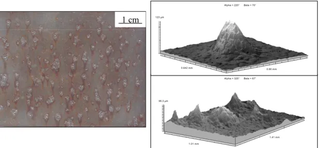
Fig. 1a shows the spatial distribution of the corrosion pits generated at the surface of the sample during this accelerated corrosion test. This observed distribution results from the random impingement of the droplets of the salt fog spraying; initiation and propagation of corrosion pits indeed is promoted at sites where the chloride concentration is higher than on the rest of the tested sample surface.
Fig.1 a) Optical macrography showing the pits formed during the accelerated corrosion test at the surface of the ferritic stainless steel sample, b) Inverted view of an isolated pit recorded by the means of a 3D roughness profilometer, c) Inverted view of a cluster of pits.
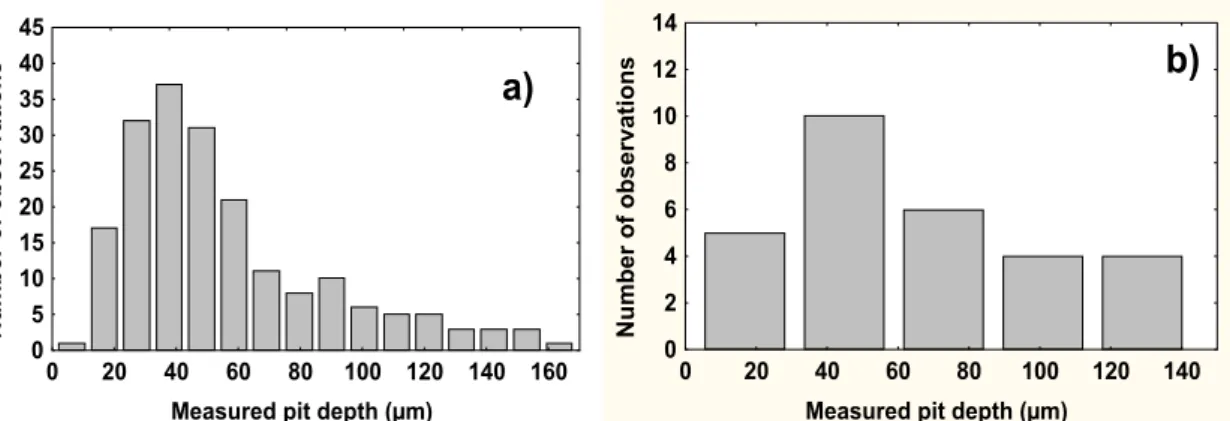
Fig. 2a shows the experimental frequency distribution of approximately 200 values of pit depth laboriously measured by the means of an optical microscope. This global distribution contains both isolated pits and clusters of pits as respectively illustrated in Fig. 1b and c. It was already shown in a previous paper that, for a limited sample of 29 isolated pits extracted from the global distribution, the pit morphology was better described by a Gaussian model rather than by a spherical shape [14]. Fig. 2b. shows the experimental pit depth frequency distribution related to these 29 isolated pits which morphology was characterised by the means of a 3D-roughness profilometer. For this limited dataset, the recorded value of the maximum pit depth is 121 µm whereas it is 165 µm in the case of the global distribution.
4
Measured pit depth (µm)
Number of observations 0 5 10 15 20 25 30 35 40 45 0 20 40 60 80 100 120 140 160 a)
Measured pit depth (µm)
Number of observat ions 0 2 4 6 8 10 12 14 0 20 40 60 80 100 120 140 b)
Fig. 2: Experimental frequency distribution of the corrosion pit depths measured by a) an optical microscope (approximately 200 pits were considered), b) a 3D-roughness profilometer (29 pits were considered).
3. Modelling of the pit depths distribution using the GLD method
The Generalized Lambda Distribution (GLD) method was used in this paper to model the experimental frequency of the corrosion pit depths presented in Fig.2b; i.e. for the limited dataset of the 29 isolated pits under consideration in this study.
3.1) Brief presentation of the GLD method [15]
The generalized lambda distribution family is specified in terms of its percentile function (called also the inverse distribution function) with four parameters λ1, λ2, λ3 and λ4:
(
y
;
λ
1,
λ
2,
λ
3,
λ
4)
λ
1(
y
λ3(
1
y
)
λ4)
λ
2Q
X=
+
−
−
(3)The parameters λ1 and λ2 are, respectively, the location and scale parameters, while λ3 and
4
λ determine respectively the skewness and the kurtosis of the GLD.
The probability density function (PDF) can then be easily expressed from the percentile function of equation (3):
( )
(
(
)
1)
4 1 3 2 3− + 1− 4− =λ λ yλ λ y λ x fX (4)Basically, the problem consists in determining the parameters λ1, λ2, λ3, λ4 which define the GLD giving the best fitting curve with the experimental frequency distribution. Dedicated to that purpose, the method of percentiles has been used to assess in a first time the following sample statistics: 5 . 0 1 ˆ ˆ π ρ = (5), ρˆ2 =πˆ1−u −πˆu (6), 5 . 0 1 5 . 0 3 ˆ ˆ ˆ ˆ ˆ π π π π ρ − − = −u u (7), u u π π π π ρ ˆ ˆ ˆ ˆ ˆ 1 25 . 0 75 . 0 4 − − = − (8)
where πˆp denotes the score indicating that 100 percent of the distribution consists of scoresp
that are smaller than that particular value and u is a number that must be chosen between 0 and 0.25. In the case of a limited dataset, as for example in this study, the authors of the method recommend to choose an intermediate value u=0.1 [15].
Then, from the definition of the GLD, Karian et al.[15] express the GLD counterparts of the above statistics as follows:
2 1 1 4 3 0.5 5 . 0 λ λ ρ = + λ − λ (9),
(
)
(
)
2 2 3 4 4 3 1 1 λ ρ = −u λ −uλ + −u λ −uλ (10),(
)
(
)
3 4 4 3 4 3 3 4 5 . 0 5 . 0 1 5 . 0 5 . 0 1 3 λ λ λ λ λ λ λ λ ρ − + − − − + − − = u u u u (11),(
)
3 4(
)
4 3 3 4 4 3 1 1 25 . 0 75 . 0 25 . 0 75 . 0 4 λ λ λ λ λ λ λ λ ρ u u u u − + − − − − + − = (12)The determination of the best fitting GLD (λ1, λ2, λ3, λ4) is performed by solving this system of 4 equations estimating ρj value by ρˆj with j∈
{
1,2,3,4}
. Since the overall system is highly non-linear, only the subsystem ρˆ3 =ρ3 and ρˆ4 = ρ4 that involves λ3 and4
λ has been solved in this study by minimising the following function thanks to a steepest gradient algorithm:
(
)
∑
(
)
= − = Ψ 4 3 2 4 3, ˆ j j j ρ ρ λ λ (13)When the values of λ3 and λ4 that minimise the above equation are found, so λ2 and λ1 can be determined using successively equations (10) and (9).
It must be outlined that the GLD have been shown to fit well many of the most important theoretical distributions including exponential type ones and that the goodness of fit was particularly significant in the right tail region; region corresponding to the extreme values [15]. Nevertheless, the main advantage of using the GLD method is that it can be applied regardless of the type of the theoretical underlying parent distribution of corrosion pit depths. 3.2) Results
The values of the percentiles related to the experimental pit depth frequency distribution of the limited dataset of 29 isolated pits under consideration in this study are reported in Table I. The values of these percentiles have been inserted in equations (5) to (8) to calculate at a first stage the values of ρˆ1, ρˆ2, ρˆ3 and ρˆ4 which are also reported in the same table.
75 . 0 ˆ π πˆ0.5 πˆ0.25 πˆ0.1 πˆ0.9 ρˆ1 ρˆ2 ρˆ3 ρˆ4 88.89 52.87 31.07 19.15 117.8 52.87 98.65 0.519 0.586
Tab. 1: Values of the percentiles of interest together with the related values of ρˆ1, ρˆ2, ρˆ3
and ρˆ4 describing the experimental limited dataset presented in Fig.2b.
At a second stage, the values of ρˆ3 and ρˆ4 have been used to calculate the values of λ3 and
4
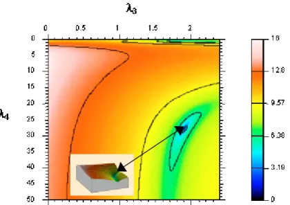
λ by solving the subsystem ρˆ3 =ρ3 and ρˆ4 =ρ4 using equations (11) to (13). These calculations were performed by the means of a computer algorithm we especially developed for this task. The numerical results of the minimisation processing are shown in Fig. 3 which presents both a 3D view and a contour plot of the values of the function Ψ
(
λ3,λ4)
for5 . 2
6
Fig. 3: Contour plot of the values of the function Ψ
(
λ3,λ4)
related to the 3D view inserted on the right bottom corner. The white arrow indicates the minimum value of the function.The minimum value of the function Ψ
(
λ3,λ4)
is found for the following pair (λ3 =2.01, 9. 27 4 =
λ ) which subsequently yields to the pair (λ1 =24.13, λ2 =0.0086) using equations (9) and (10). Inserting these four values in equation (4) then enables to express formally the probability density function that gives the best fitting curve with the experimental frequency distribution. This best fitting probability density function is plotted in Fig. 4.
Fig.4: Probability density function corresponding to Eq. (4) for parameters (λ1 =24.13, 0086
. 0 2 =
λ , λ3 =2.01, λ4 =27.9)
4. Prediction of the maximum pit depth combining the GLD and the Bootstrap methods
The Computer-Based Bootstrap Method (CBBM) was used in this study to assess the influence of a perturbation in the scores of the experimental dataset (which is limited) on the shape (that depends on the estimation of the parameters λ1, λ2, λ3 and λ4 values) of the resulting probability function determined by applying the GLD method and the related variability of the predicted maximum pit depth.
Pit depth (µm) Probability density 0 0.004 0.008 0.012 0.016 0.02 0 20 40 60 80 100 120 140
4.1) Brief presentation of the Computer-Based Bootstrap Method [16, 17]
Based on the mathematical resampling technique, the main principle of the CBBM consists in generating a high number I of simulated Bootstrap samples from the original dataset using
the power of a modern computer. The original dataset consists of either experimental or simulated scores. A Bootstrap sample i
(
i∈[1 to I])
of size n, noted ( 1, 2,..., i)n i
i p p
p , is a
collection of n values simply obtained by randomly sampling with replacement from the original data scores (p1,p2,...,pn), each of them having a probability equal to n1 to be selected. A Bootstrap sample contains therefore scores of the original dataset; some appearing zero times, some appearing one, some appearing twice, etc.
4.2) Procedure and results
A Bootstrap algorithm was computed to generate I =100 simulated Bootstrap samples of size n=29 from the 29 experimental values of isolated pit depth under consideration in this study. For each simulated Bootstrap sample i
(
i∈[ to1 100])
, new values of the parameters noted i 1 λ , i 2 λ , i 3 λ and i 4λ are then determined (by using the method described in part 3) to obtain a new GLD (i i 1 λ , i 2 λ , i 3 λ , i 4
λ ) that will be called a ‘Bootstrapped GLD’.
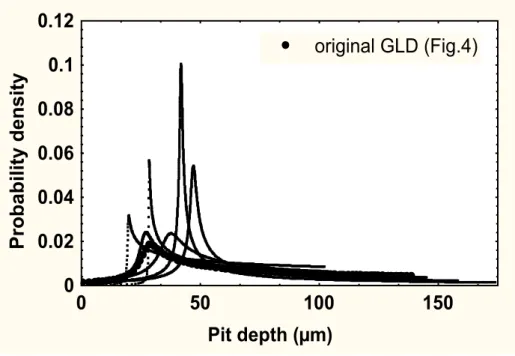
To illustrate the result of this procedure, an example of six Bootstrapped GLDs related to six Bootstrap samples are presented in Fig. 5. These probability density functions resulting from the combination of the CBBM and the GLD methods simulate in fact perturbed distributions of pit depth equivalent to the experimental one.
Fig. 5: Six examples of Bootstrapped probability density functions obtained by processing six Bootstrap samples using the GLD method.
The equation of a given cumulative Bootstrapped GLD (i i
1 λ , i 2 λ , i 3 λ , i 4 λ ) is:
( )
i(
(
)
)
i i i iy
y
y
p
=
λ
1+
λ3−
1
−
λ4λ
2 (14) Pit depth (µm) Probability density 0 0.02 0.04 0.06 0.08 0.1 0.12 0 50 100 150 original GLD (Fig.4)8
where y is a uniform random number between 0 and 1 and
p
i( )
y
is the simulated corrosion pit depth related to this number.For each Bootstrap GLD (i i
1 λ , i 2 λ , i 3 λ , i 4
λ ), the CBBM was used again to generate J =5000 Bootstrap samples of size n=29 using equation (14). The highest score i
j
x (i.e. the maximum simulated pit depth) of each Bootstrap sample j
(
j∈[1 to 5000])
related to the Bootstrap GLD (i i 1 λ , i 2 λ , i 3 λ , i 4λ ) is then retained giving finally a set of 500000 extreme values when i varies from 1 to 100. Fig. 6 shows the Bootstrapped distribution of this set of maximum pit depth from which traditional statistic estimates like the mean and the 90% symmetrical confidence interval (i.e. the difference between the 95th and the 5th percentiles) can be easily determined to assess respectively the central tendency and the dispersion.
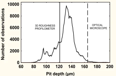
Fig. 6: Bootstrapped probability density function of the 500000 extreme pit depths extracted from the 500000 simulated Bootstrap samples. The full vertical line added on this figure call back the maximum value of the limited dataset (29 values of pit depths measured by the means of a 3D-roughness profilometer) and the dashed one the maximum value of the global distribution (approximately 200 values of pit depths measured by the means of an optical microscope).
The calculated mean of the pit depth extreme values is 129 µm and 90% of these extreme values lie between 98 µm and 153 µm. It is very interesting to note that the maximum value of corrosion pit depths assessed in the case of the global distribution (characterised by the means of an optical microscope) is accurately predicted by applying our methodology to a limited dataset (characterised by the means of a 3D roughness profilometer.
5. Conclusions
A new and alternative methodology to the Gumbel approach was presented in this paper with a view towards predicting from a limited inspection data the maximum depth of pits that propagated on a sample of ferritic stainless steel during an accelerated corrosion test.
Pit depth (µm) Number of observations 0 2000 4000 6000 8000 10000 60 80 100 120 140 160 180 200 OPTICAL MICROSCOPE 3D ROUGHNESS PROFILOMETER
Based on the power of modern computer, this methodology combines two recent statistical methods that can be applied regardless of the type of the theoretical underlying parent distribution of pit depths: the first one, the Generalized Lambda Distribution method, was used to model the distribution of pit depths and the second one, the Computer-Based Bootstrap Method, to simulate distributions of corrosion pit depths equivalent to the experimental one and to predict the maximum pit depth from the limited dataset under study. The application of this methodology to this limited dataset leads to an accurate prediction of the maximum value observed in a larger dataset.
While corrosion pits have been generated in an atmospheric environment in this study, the alternative methodology presented in this paper is thought to be also applicable for pits generated in aqueous solutions since it only necessitates the knowledge of the distribution of a morphological feature (i.e. pit depth). Such a methodology, which is aimed to improve maintenance procedures in the field of corrosion, can be also applied to any kind of defects like inclusions or pores existing in the microstructure of engineering materials.
6. References
1. T. Shibata, ISIJ Int., 31 (1991), 115.
2. A. Turnbull, Brit. Corros. J., 28 (1993), 297.
3. S. Khomukai and K. Kasahara, J. Res. Natl. Inst. Stand. Tech., 99 (1994), 321. 4. T. Shibata, Corrosion, 52 (1996), 813.
5. Y. Ishikawa, T. Ozaki, N. Hosaka and O. Nishida: Trans. ISIJ, 22 (1982), 977. 6. S. Yamamoto and T. Sakauchi, Int. J. Mater. Prod. Tech., 6 (1991), 37.
7. J.W. Provan and E.S. Rodriguez, Corrosion, 45 (1989), 179.
8. A.K. Sheikh, J.K. Boah and D.A. Hansen, Corrosion, 46 (1990), 190. 9. A.K. Sheikh, J.K. Boah and M. Younas, Rel. Eng. Sys. Saf., 25 (1989), 1. 10. E. Sato and T. Murata, Nippon Steel Technical Report, 32 (1987), 54.
11. E.J. Gumbel, “Statistical Theory of Extreme Values and Some Practical Applications”, Applied Mathematics Series 33, National Bureau of Standards, Washington, D.C., (Feb. 1954).
12. D. Najjar, M. Bigerelle, C. Lefebvre and A. Iost, ISIJ Int., 43 (2003), 720.
13. L. Bourdeau and A. Jussiaume, Proceedings of the conference Euroccor’97, Trondheim, Norway, vol II (1997), 503.
14. D. Najjar, C. Lefebvre, L. Bourdeau, M. Bigerelle and A. Iost, Proceedings CDR of the conference MATERIAUX 2002, Tours, France, (2002), Paper AF05006.
15. Z.A. Karian and E.J. Dudewicz, “Fitting Statistical Distributions, The Generalized Lambda Distribution and Generalized Bootstrap Methods”, ed. Chapman & Hall, CRC Press, Boca Raton, Florida (2000).
16. B. Efron, Ann. Stat., 7 (1979), 1.
17. B. Efron and R. Tibshirani, “An Introduction to the Bootstrap”, Chapman & Hall, New York (1993).