is an open access repository that collects the work of Arts et Métiers Institute of
Technology researchers and makes it freely available over the web where possible.
This is an author-deposited version published in: https://sam.ensam.eu
Handle ID: .http://hdl.handle.net/10985/7816
To cite this version :
Thomas HENNERON, Stéphane CLENET - Model Order Reduction of Non-Linear Magnetostatic Problems Based on POD and DEI Methods - IEEE transactions on Magnetics - Vol. 50, n°2, p.n.c. - 2014
Any correspondence concerning this service should be sent to the repository Administrator : [email protected]
M
ODEL
O
RDER
R
EDUCTION OF
N
ON
-L
INEAR
M
AGNETOSTATIC
P
ROBLEMS BASED ON
POD
AND
DEI
M
ETHODS
T. Henneron
1and S. Clénet
21L2EP/Université Lille1, Cité Scientifique - 59655 Villeneuve d’Ascq, France
2 L2EP/Arts et Métiers ParisTech, Centre de Lille, 8 boulevard Louis XIV - 59046 Lille Cedex, France
In the domain of numerical computation, Model Order Reduction approaches are more and more frequently applied in mechanics and have shown their efficiency in terms of reduction of computation time and memory storage requirements. One of these approaches, the Proper Orthogonal Decomposition (POD), can be very efficient in solving linear problems but encounters limitations in the non-linear case. In this paper, the Discret Empirical Interpolation Method coupled with the POD method is presented. This is an interesting alternative to reduce large-scale systems deriving from the discretization of non-linear magnetostatic problems coupled with an external electrical circuit.
Index Terms— Discret Empirical Interpolation Method, Model Order Reduction, Non-linear Problem, Proper Orthogonal
Decomposition, Static fields.
I. INTRODUCTION
O DESCRIBE the behavior of electrical machines coupled with an external electrical circuit, the Finite Element Method associated with a time-stepping scheme is often used to numerically solve Maxwell’s equations coupled with the circuit equations. When a fine mesh and a small time step are used, the computation time of the large-scale system obtained from the discretization of the Non-Linear Partial Differential Equations (NL-PDE) can be prohibitive. To tackle this issue, an alternative method is to apply model order reduction methods. In the literature, the Proper Orthogonal Decomposition has been widely used to solve many problems in engineering [1]. This method consists of performing a projection onto a reduced basis, meaning the size of the equation system to solve can be highly reduced. The snapshot approach is the most popular to determine the discrete projection operator between the original basis (generating from the mesh) and the reduced basis [2]. In computational electromagnetics, the POD method has been applied to study the behavior of a transformer with a non-linear core [3][4] or to solve magnetoquasistatic and electroquasistatic field problems [5][6]. In the case of linear PDEs, the POD approach can lead to a dramatic reduction in the computation time. In the non-linear case, this method is not quite as efficient due to the computation cost of the non-linear terms in the reduced system, which requires the assembling of the equation system of the full initial problem. To tackle this issue, the Discret Empirical Interpolation Method (DEIM) method can be coupled with the POD approach [7]. DEIM interpolates the non-linear behavior of the magnetic field on the whole spatial domain from evaluations of the non-linear behavior law on a reduced number of localized regions. The determination of such localized regions is automatic and does not require any intervention from the user. The computation time of the non- linear terms when applying the POD is thus highly reduced.
In this paper, the DEIM-POD approach is applied to solve a
non-linear magnetostatic problem coupled with an electrical circuit using the vector potential formulation. First, the numerical model is presented. Secondly, the Snapshot POD method and the DEIM are developed. Finally, non-linear models based solely on either the POD method or the DEIM-POD are compared. The results obtained with the reduced models are also compared in terms of accuracy and computation time using the full Finite Element model.
II. NON-LINEAR MAGNETOSTATIC PROBLEM COUPLED WITH ELECTRIC CIRCUIT
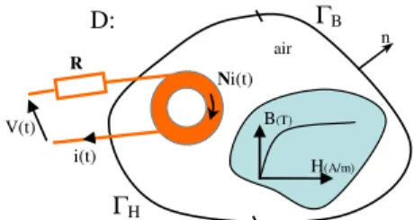
Let us consider a domain D of boundary Γ (Γ=ΓB∪ΓH and
ΓB∩ΓH=0) (Fig. 1). The problem is solved on D×[0,T] with T the width of the time interval. The source field is created by a stranded inductor supplied by a voltage v(t).
ΓB ΓH D: B(T) H(A/m) V(t) Ni(t) i(t) air R n
Figure 1. Non-linear magnetostatic problem coupled with electrical circuit In magnetostatics, the problem can be described by the following equations: curl H(x,t) = N(x)i(t) div B(x,t) = 0 H(x,t) = ν(B) (x)B(x,t) (1) (2) (3) with B the magnetic flux density, H the magnetic field, N and i the unit current density and the current flowing through the stranded inductor and finally ν(B) (x) the reluctivity. For
the ferromagnetic material, ν(B) (x) may depend on B in the
non-linear case. To impose the uniqueness of the solution, boundary conditions must be added such that:
B(x,t).n=0 on ΓB and H(x,t)×n=0 on ΓH (4)
T
Manuscript received January 1, 2008 (date on which paper was submitted for review). Corresponding author: T. Henneron (e-mail: [email protected]).
with n the outward unit normal vector. In order to impose the voltage v(t) at the terminals of the stranded inductor, the following relation must be considered:
v(t) Ri(t) dt
(t)
dΦ + = (5)
with R the resistance of the inductor and Φ the flux linkage. The previous problem can be solved by introducing the vector potential A. From (2), this potential is defined such that B(x,t)=curlA(x,t) with A(x,t)××××n=0 on ΓB. To take into account the non-linear behavior of the ferromagnetic material, the fixed point technique can be used [8]. In this case, the magnetic field H(x,t) can be expressed by H(x,t)=νfpB(x,t)+Hfp(B(x,t)) with νfp a constant and
Hfp(B(x,t))=(ν(B) (x)-νfp)B(x,t) a virtual magnetization vector.
According to (1) and (5), the equations to solve are t))) , ( ( ( -)i(t) ( t)) , (
( fpcurlA x N x curl Hfp curlAx
curlν − = , (6) v(t) Ri(t) )dD ( t). , ( dt d D = +
∫
Ax Nx . (7) To ensure the unicity of the solution, a gauge condition must be added. To solve this problem, A(x,t) and N(x) are discretised using edge and facet elements [9]. We denote Ai(t)the value of A along the ith edge and Ne the number of edges.
Then, applying the Galerkin method to (6) and (7), a system of differential algebraic equations is obtained
(t)) ( (t) dt (t) d (t) K X F Mfp X MX + = − (8)
with X(t) the vector of unknowns of size Nun=Ne+1 such
that (Xi(t))1≤i ≤Ne =(Ai(t)) 1≤i ≤Ne and XNun(t) = i(t). M and K are
Nun×Nun matrices and F(t) and Mfp(X(t)) Nun×1 vectors.
III. MODEL ORDER REDUCTION WITH DEIM-POD
A. Proper Orthogonal Decomposition
In order to reduce the computation time required to solve system (8), the POD method is applied [1]. The vector X(t) is approximated in a reduced basis by a vector Xr(t) of size Ns
(Ns<<Num). To obtain a discrete projection operator ΨΨΨΨ such
that
(t) (t) ΨXr
X = , (9)
the snapshot approach is typically applied [2]. The system (8) is solved for the first Ns time steps (called snapshots). The
snapshot matrix Ms is defined by Ms=(Xj)1≤j≤Ns with Xj the
solution X(t) at the jth time step. Applying the Singular Value Decomposition (SVD), Ms can be decomposed under the
form:
Ms=VΣΣΣΣWt (10)
with VNun×Nun and WNs×Ns orthogonal matrices and ΣΣΣΣNun×Ns
the diagonal matrix of the singular values. The ith row of W represents the entries of the ith vector of the matrix Ms
projected in the reduced basis formed by the Ns vectors of the
matrix VΣΣΣΣ. The operator ΨΨΨ is then given by normalizing the Ψ matrix VΣΣΣΣ or MsW. Finally, in the reduced basis, the new
system to solve can be deduced combining (8) and (9)
(t)) ( (t) dt (t) d (t) r t t fp r r r r ψF ψM ΨX X K X M + = − with M =ΨtMΨ r and K ΨKΨ t = r . (11)
In practical terms, the computational time of the SVD of Ms
can be prohibitive due to its size which depends on Nun and
Ns. To tackle this issue, the matrix of correlations Cs of Ms is
used. This matrix is determined such that
s t s s s N 1 M M C = (12)
The size of Cs is Ns×Ns. The eigenvalue decomposition of
Cs can be applied to obtain the matrix W because Cs = WΣΣΣΣVt
VΣΣΣΣWt= W∆∆∆∆Wt. In this case, the complexity and the computational time to determine W is highly reduced compared to a SVD of Ms.
B. Discret Empirical Interpolation Model with POD
In the non-linear case, the computational complexity of the vector fnl(t) = Mfp(ΨΨΨΨXr(t)) can be significant (see (12)). In fact,
it is necessary to evaluate the solution X(t)=ΨΨΨΨXr(t) in the original basis to determine the vector Mfp(X(t)). To tackle this
issue, an alternative is to apply the DEIM [7]. This approach proposes to approximate the non-linear function fnl(t) by
combining projections with interpolations. All the entries of the vector fnl(t) no longer need to be evaluated. The
approximation of fnl(t) is determined from a linear
combination of a limited number entries of fnl(t) selected
automatically applying the DEIM. The jth entry fnlj(t) of the
vector fnl(t) is equal to the integral over the domain of curl Hfp
weighted by the edge shape function wj. Since wj is null
except on the elements connected to the jth edge denoted by supp{j}, the calculation of fnlj(t) is local just requiring the
circulations of A along the edges belonging to the jth edge to be able to evaluate Hfp everywhere on supp{j}. For this
reason, the calculation of this selected terms of fnl(t) is then
very fast. We seek to approximate fnl(t) by
(t)) (
(t) r
nl Uc X
f = (13)
with c(Xr(t)) the interpolation vector of size Ndeim×1 and U
an orthogonal Num×Ndeim matrix calculated by applying a POD
method with the vectors Mfp(X(t)) on the Ndeim first time steps.
The system (13) is over-determined. To express the coefficients of c(Xr(t)), Ndeim distinct rows from the
over-determined system are selected by applying a matrix P such as Ptfnl(t)= PtUc(Xr(t)). The algorithm presented in [7] is used to
determine the matrix P=(Ii)1≤i≤Ndeim with Ii a column of the
identity matrix INun×Nun. The DEIM algorithm thus extracts a
set of indices which correspond to the DEIM edges. Then, c(t) can be expressed by
Moreover, in the case of a non-linear magnetostatic problem coupled with an electrical circuit, it can be shown that, in (14), the vector PtMfp(ΨΨΨΨXr(t)) is equivalent to Mfp(PtΨΨΨΨXr(t)).
Finally, by combining (13) and (14), the vector fnl(t) is
approximated by (t)) ( ) ( (t)) ( (t) fp t 1 fp t t r nl M X UP U M P ΨX f = ≈ − (15)
In this expression, the calculation of the term Mfp(PtΨΨΨΨXr(t))
simply requires the evaluation at the Ndeim DEIM edges of the
non-linear function, and not at all edges, as in (11), to interpolate the term Mfp(X(t)). In practical terms, the term
Ψ ΨΨ
ΨtU(PtU)-1 is only calculated once. IV. APPLICATION
A 3D magnetostatic example, made of a single phase EI transformer at no load supplied at 50Hz with a sinusoidal voltage, is studied. Due to the symmetry, only one eighth of the transformer is modeled (Fig. 2). The non-linear magnetic behavior of the iron core is considered. The 3D spatial mesh is made of 12659 nodes and 67177 tetrahedrons. The Euler scheme is used to solve (11) with 30 time steps per period.
0 0,4 0,8 1,2 1,6 2 0 1000 2000 3000 4000 5000 6000 H(A/m) B(T)
Figure 2. Example of application (a: geometry, b: non-linear curve of the core) In the following, we compare the results obtained from the POD and DEIM-POD reduced models with those obtained using the full model. The solution given by the full model will be considered as the reference.
A. Influence of the number of snapshots on the evolution of the current
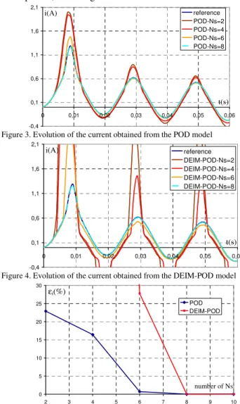
In order to evaluate the influence of the number of snapshots on a global value, the evolutions of the current i(t) versus time, obtained from the POD and DEIM-POD models, are compared with the reference in Fig. 3 and Fig. 4. The Ns
snapshots correspond to the vector A for the Ns first time steps
of the full model. The size of the reduced model (11) is equal to the number of snapshots. The reduced model is then run again starting at t=0. The number of snapshots influences the evolution of the current for both reduced models. The POD models as expected gives the same results as the full model for the Ns first time step and then it appears a divergence. This
property is not satisfies anymore with the DEIM-POD method since the non-linearity is not accounted as in the full model. We can observe that the current waveform converges towards the reference with both approaches when Ns increases. In
order to estimate the convergence versus the number of snapshots, an error estimator εi is defined
2 ref 2 red ref i ε i i i − = (16)
with iref and ired the vectors of current values at each time
step obtained from the reference and the POD (or DEIM-POD) model respectively. Figure 5 presents the evolution of εi
versus the number of snapshots. We can see that the convergence is faster with POD where the non-linear vector Mfp in (11) is evaluated for all edges of the mesh. In the case
of the DEIM-POD model, this vector is interpolated with a low number of edges using (15). In our case, the number of DEIM edges is equal to the number of snapshots. Then, the number of DEIM edges must be sufficient to obtain a good interpolation of the vector Mfp(ΨΨΨΨXr(t)). This vector is
correctly expressed with 8 DEIM edges. The error on the current is equal to 0.03%. For the same number of snapshots, the error is 0.004% for the POD model. The DEIM-POD approach requires more snapshots to obtain a result very close to that of the reference than the POD model. Figure 6 presents the edges selected automatically by the DEIM for 8 snapshots. As expected, these edges are located in the saturated area.
-0,4 0,1 0,6 1,1 1,6 2,1 0 0,01 0,02 0,03 0,04 0,05 0,06 t(s) i(A) reference POD-Ns=2 POD-Ns=4 POD-Ns=6 POD-Ns=8
Figure 3. Evolution of the current obtained from the POD model
-0,4 0,1 0,6 1,1 1,6 2,1 0 0,01 0,02 0,03 0,04 0,05 0,06 t(s) i(A) reference DEIM-POD-Ns=2 DEIM-POD-Ns=4 DEIM-POD-Ns=6 DEIM-POD-Ns=8
Figure 4. Evolution of the current obtained from the DEIM-POD model
0 5 10 15 20 25 30 2 3 4 5 6 7 8 9 10 number of Ns POD DEIM-POD εi(%)
Figure 5. Error of the current versus the number of snapshots
magnetic core
prim ary winding secondar y winding
DEIM edge
(a) (b)
Figure 6. DEIM edges in the magnetic core (a: 3D view, b: view of top)
B. Influence of the number of snapshots on the distribution of the fields
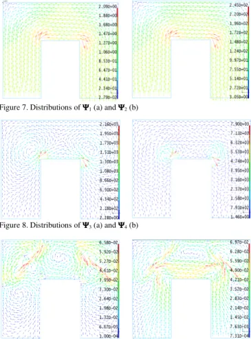
According to (9), the vector solution is approximated by a linear combination of vector ΨΨΨΨj of ΨΨΨ, often called a mode. Ψ Each ΨΨΨΨj corresponds to a field distribution. Figures 7 and 8 present the field distribution corresponding to ΨΨΨΨj for the first four modes in the magnetic core. The distribution corresponding to ΨΨΨΨ1 and ΨΨΨΨ2 are close to a physical distribution of the magnetic flux density encountered in a transformer. The distributions corresponding to ΨΨΨΨ3 and ΨΨΨΨ4 have no physical meaning except that they enable us to better take into account the saturation at the corner of the core.
Figure 7. Distributions of ΨΨΨΨ1 (a) and ΨΨΨΨ2 (b)
Figure 8. Distributions of ΨΨΨΨ3 (a) and ΨΨΨΨ4 (b)
Figure 9. Distribution of the difference between the magnetic flux density obtained by the reference model and the POD (a) and DEIM-POD (b) (t=10ms)
In figure 9, the error of the distribution determined with the POD and DEIM-POD models for 8 snapshots are given. Their distributions express the truncation of the solution between the
reference model and the reduced models. If we increase the number of snapshots, the error will decrease. We can observe that the distributions of the error are different between the POD and DEIM-POD models. This difference can be explained by the interpolation of the non-linear term in the case of the DEIM-POD model.
C. Computation time
In terms of computation time, with a time interval width of 0.12s and 120 time steps, the reference model requires 130min. For 8 snapshots, the computation time is 24min with the POD and 11min with the DEIM-POD. These computation times do not take into account the computation time required to evaluate the solutions of the snapshots: for 8 snapshots, the computation time is 8min42s. The DEIM-POD model is faster than the POD model, the ratio being 2.2. This ratio is a function of the number of elements in the magnetic core. With a finer mesh and a fixed number of snapshots, the computation time required to evaluate the non-linear term Mfp(ΨΨΨΨXr(t)) in
(11) is more significant and thus, the computation time ratio for the non-linear term between the POD and DEIM-POD models increases.
V. CONCLUSION
The Proper Orthogonal Decomposition and the Discret Empirical Interpolation Method associated with a FEM vector potential formulation have been developed in order to solve a 3D non-linear magnetostatic problem coupled with an external circuit. Based on the example here, it has been shown that the POD model associated with the DEIM enables us to reduce the computation time significantly while obtaining good precision. In this paper, the fixed point technique has been used to account for the non linearity. Future work will be to extend the application of the POD-DEIM when the Newton Raphson method is applied.
REFERENCES
[1] J. Lumley, “The structure of inhomogeneous turbulence”, Atmospheric
Turbulence and Wave Propagation. A.M. Yaglom and V.I. Tatarski., pp. 221–227, 1967.
[2] L. Sirovich, “Turbulence and the dynamics of coherent structures”, Q.
Appl. Math., vol. XLV, no. 3, pp. 561–590, 1987.
[3] Y. Zhai, “Analysis of Power Magnetic Components With Nonlinear Static Hysteresis: Proper Orthogonal Decomposition and Model Reduction”, IEEE Trans. Magn., vol. 43(5), pp. 1888-1897, 2007. [4] T. Henneron, S. Clénet, “Model Order Reduction of Electromagnetic
Field Problem Coupled with Electric Circuit Based on Proper Orthogonal Decomposition”, Proceeding of OIPE (Ghent), 2012. [5] D. Schmidthäusler, M. Clemens, “Low-Order Electroquasistatic Field
Simulations Based on Proper Orthogonal Decomposition”, IEEE Trans.
Magn., vol. 48(2), pp. 567-570, 2012.
[6] T. Henneron, S. Clénet, “Model order reduction of quasi-static problems based on POD and PGD approaches”, EPJ AP, to be published. [7] S. Chaturantabut and D. C. Sorensen, “Nonlinear Model Reduction via
Discrete Empirical Interpolation”, SIAM J. Sci. Comput., vol. 32(5), pp.2737–2764, 2010.
[8] M. Chiampi, D. Chiarabaglio, M. Repetto, “A jiles-Atherton and Fixed-point Combined Technique for Time Periodic Magnetic field Problems with Hysteresis”, IEEE Trans. Magn..vol. 31(6), pp 4306-4311, 1995. [9] A. Bossavit, “A rationale for edge-elements in 3-D fields computations”,