2019 — Nonlinear control and perturbation compensation in UAV quadrotor
Texte intégral
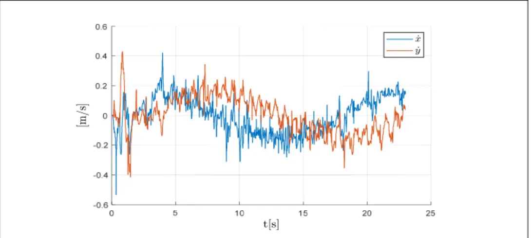
Figure


Documents relatifs
Abstract— This paper presents a bounded formation con- troller for multiple quadrotors (UAVs) system with leader- follower structure.. Considering the actuator saturation of
Zusammenfassung Der Beitrag beschreibt den Entwurf eines nichtlinearen Flugreglers für ein vierrotoriges unbemanntes Fluggerät,einensogenannten Quadrocopter.Dievorgeschlagene
CONCLUSIONS AND FUTURE WORKS This paper presents a vehicle control system for a quadro- tor Micro-UAV based on a combined control strategy in- cluding feedback linearization to
The second task of the overall landing controller comprises the tracking of the image of the moving platform with the quadrotor in a pure x-y-plane and to control the quadrotor in a
In order to evaluate the vehicle control system, an experimental prototype of the quadrotor has been designed (see Fig. 1), the dynamic model has been derived by identification of
In order to evaluate the derived vehicle and landing control system, an experimental prototype of the quadrotor has been designed and the dynamic model (6) of this quadrotor has
CONCLUSIONS AND FUTURE WORKS This paper presents a vehicle control system for a small quadrotor UAV based on the state-dependent Riccati equation controller (SDRE).. Both an
Copyright and moral rights for the publications made accessible in the public portal are retained by the authors and/or other copyright owners and it is a condition of
