Science Arts & Métiers (SAM)
is an open access repository that collects the work of Arts et Métiers Institute of Technology researchers and makes it freely available over the web where possible.
This is an author-deposited version published in: https://sam.ensam.eu Handle ID: .http://hdl.handle.net/10985/10208
To cite this version :
Badis HADDAG, Farid ABED-MERAIM, Tudor BALAN - Strain localization analysis using a large deformation anisotropic elastic-plastic model coupled with damage - International Journal of Plasticity - Vol. 25, n°10, p.1970-1996 - 2009
Any correspondence concerning this service should be sent to the repository Administrator : [email protected]
Accepted Manuscript
Strain localization analysis using a large deformation anisotropic elastic-plastic model coupled with damage
Badis Haddag, Farid Abed-Meraim, Tudor Balan
PII: S0749-6419(08)00191-5
DOI: 10.1016/j.ijplas.2008.12.013
Reference: INTPLA 1208
To appear in: International Journal of Plasticity Received Date: 29 July 2008
Revised Date: 1 December 2008 Accepted Date: 21 December 2008
Please cite this article as: Haddag, B., Abed-Meraim, F., Balan, T., Strain localization analysis using a large deformation anisotropic elastic-plastic model coupled with damage, International Journal of Plasticity (2008), doi: 10.1016/j.ijplas.2008.12.013
This is a PDF file of an unedited manuscript that has been accepted for publication. As a service to our customers we are providing this early version of the manuscript. The manuscript will undergo copyediting, typesetting, and review of the resulting proof before it is published in its final form. Please note that during the production process errors may be discovered which could affect the content, and all legal disclaimers that apply to the journal pertain.
ACCEPTED MANUSCRIPT
Strain localization analysis using a large deformation anisotropic
elastic-plastic model coupled with damage
Badis Haddag, Farid Abed-Meraim* and Tudor Balan
Laboratoire de Physique et Mécanique des Matériaux, LPMM, UMR CNRS 7554, ENSAM de Metz, Arts et Métiers ParisTech, 4 rue Augustin Fresnel, 57078 Metz Cedex 3, France
Keywords: Strain Localization, Anisotropic Elastic-plasticity, Large Strain,
Isotropic-Kinematic Hardening, Continuum Damage Theory, Shear Band, Finite Element Simulation.
* Corresponding author. Address: ENSAM de Metz, 4 rue Augustin Fresnel, 57078 Metz Cedex 03, France. Tel.: +(33) 3.87.37.54.79; Fax: +(33) 3.87.37.54.70.
ACCEPTED MANUSCRIPT
2
Abstract
Sheet metal forming processes generally involve large deformations together with com-plex loading sequences. In order to improve numerical simulation predictions of sheet parts forming, physically-based constitutive models are often required. The main objective of this paper is to analyze the strain localization phenomenon during the plastic deformation of sheet metals in the context of such advanced constitutive models. Most often, an accurate prediction of localization requires damage to be considered in the finite element simulation. For this pur-pose, an advanced, anisotropic elastic-plastic model, formulated within the large strain framework and taking strain-path changes into account, has been coupled with an isotropic damage model. This coupling is carried out within the framework of continuum damage me-chanics. In order to detect the strain localization during sheet metal forming, Rice’s localiza-tion criterion has been considered, thus predicting the limit strains at the occurrence of shear bands as well as their orientation. The coupled elastic-plastic-damage model has been imple-mented in Abaqus/Implicit. The application of the model to the prediction of Forming Limit Diagrams (FLDs) provided results that are consistent with the literature and emphasized the impact of the hardening model on the strain-path dependency of the FLD. The fully three-dimensional formulation adopted in the numerical development allowed for some new results – e.g. the out-of-plane orientation of the normal to the localization band, as well as more real-istic values for its in-plane orientation.
ACCEPTED MANUSCRIPT
3
1. Introduction
The numerical prediction of metal forming defects is a constant preoccupation both for scientists and industry. With the development of new grades of sheet metals with high per-formances (i.e. combining large ductility with high strength), the study of their formability limits has become of great importance, since it contributes to increasing the design efficiency by reducing costs and time. In order to characterize the formability of sheet metals, Keeler (1965) introduced the concept of Forming Limit Diagram, which is defined by the two values of the principal strains in the sheet plane. This diagram represents a real practical interest, in the sense that it defines a safe zone corresponding to the domain of the sheet formability. Since this early work of Keeler, several efforts have been devoted to the prediction of such diagrams (e.g. Laukonis and Gosh, 1978; Hutchinson and Neale, 1978; Cordebois and Ladevèze, 1982; Needleman and Tvergaard, 1983; Brunet et al., 1985; Arrieux et al., 1985; Kuroda and Tvergaard, 2000a,b; Stoughton, 2000; Chow et al., 2002, Butuc et al., 2006).
The use of advanced constitutive models is known to contribute to the proper prediction of the stress/strain history of the material under complex loading and, thus, to an improved pre-diction of the formability limit. The accurate description of the material behavior has received considerable attention in the last decades. For simple applications, the Swift and Voce laws are widely used to reproduce the isotropic hardening that occurs during monotonic loading paths. However, strain-path changes induce more complex phenomena that must be consid-ered in the constitutive model. Among the phenomenological approaches, more advanced models are defined by combining isotropic and kinematic hardening. In these models, several internal variables with nonlinear evolution laws are introduced in order to improve the de-scription of the Bauschinger effect, the ratcheting effect in fatigue, etc. (e.g. Marquis, 1979; Chaboche, 1986; Lemaitre and Chaboche, 1985). An extensive bibliography on this subject is reported in (Haddag et al., 2007) as well as in (Chaboche, 2008).
Since hardening in sheet metals is essentially due to the dislocation microstructure and its evolution, numerous attempts have been made to describe its effect on hardening at a macro-scopic scale. Following this approach, Teodosiu and Hu (1995, 1998) and Teodosiu (1997) proposed a microstructure-based model representing not only the monotonic or reverse load-ing, but also the whole range between the two, including the particular case of an orthogonal strain-path. More precisely, the introduction of physically-motivated internal variables that describe the evolution of the persistent dislocation structures allowed new transient
phenom-ACCEPTED MANUSCRIPT
4
ena to be modeled. Stagnation, softening, and rapid changes in the work hardening rate – as observed during abrupt, two-stage sequential rheological tests – for a wide range of sheet metals are very well described with this model (Haddadi et al., 2006). In the current work, the plastic anisotropy induced by hardening has been modeled with the Teodosiu and Hu (1998) hardening model. The model can be coupled with any yield potential to take into account ini-tial anisotropy. The classical cyclic hardening model of Chaboche, combining the Armstrong-Frederick and Voce (or Swift) laws, is used as a reference model, since it is widely available in commercial finite element codes.
However, sheet metal forming involves large plastic deformation that may induce damage, eventually leading to strain localization when material failure is approached. In order to take this phenomenon into account, several theories have been proposed by introducing damage in the constitutive models. The most often used approaches can be classified into two categories: micromechanics-based damage formulations and continuum damage theories.
Well-established examples of each category are Gurson’s damage theory (Gurson, 1977) and the Continuum Damage Mechanics (CDM), popularized by Lemaitre (1985). The first approach consists in describing the material degradation by an internal variable representing the volume fraction of the micro-cavities formed during loading. This approach is widely applied for po-rous materials (Gurson, 1977; Benallal and Comi, 2000; etc.), as well as for sheet metals (e.g. Brunet and Morestin, 2001). On the other hand, the CDM approach introduces an internal variable that represents the surface density of micro-cracks. It is based on the thermodynamics of the irreversible processes, and is widely applied to metallic materials (Lemaitre and
Chaboche, 1985; Kachanov, 1986; Murakami, 1988; Lemaitre, 1992; Voyiadjis and Kattan, 1992a,b; Chaboche, 1999). A comparative study of different ductile models (Lemaitre and Chaboche, 1985; Gurson, 1977; Thomason, 1990; etc) can be found in Pardoen et al. (1998). The CDM approach is adopted in this paper to couple the elastic-plastic model to damage. More specifically, the Teodosiu-Hu hardening model is coupled with a Lemaitre-type damage model. This allows one to simultaneously reproduce strain-path changes and softening effects.
In order to define an intermediate state corresponding to the strain localization during loading, several approaches have been developed in the literature. Some of them are widely applied to determine the FLDs. During the last century, numerous criteria of plastic instabili-ties have been proposed, e.g. maximum load criteria (Considère, 1885; Swift, 1952; Hora et al., 1996; Brunet and Morestin, 2001), Hill’s material stability analysis (Hill, 1952 and 1958), or models assuming an initial defect in the material (Marciniak and Kuczy ski, 1967). More
ACCEPTED MANUSCRIPT
5
pragmatic models (e.g. the Marciniak-Kuczy ski model) have been given extensive attention because of their industrial applications, in spite of their weaker theoretical foundations (e.g. Kuroda and Tvergaard, 2000a,b, 2004; Aretz, 2008). On the other hand, the theoretically sounder approaches, e.g. Rice’s strain localization criterion (Rudnicki and Rice, 1975; Rice, 1976) have mainly been investigated analytically, for simpler constitutive models and for par-ticular (plane stress or plane strain) loading situations (Bigoni and Hueckel, 1991; Doghri and Billardon, 1995; Benallal and Comi, 2000; Benallal and Bigoni, 2004).
In his initial analysis of localized necking, Hill (1952) used a simple constitutive model (rigid-plastic, J2 flow theory) with a plane stress condition, showing that localized necking of
a thin sheet occurs along the line of minimum straining. As an improvement, Benallal (1998) proposed a three-dimensional analysis of localized necking by studying the properties of the plastic hardening modulus at the point of strain localization with J2 elastic-plastic flow theory.
Dudzinski and Molinari (1991) proposed a linear perturbation analysis as an alternative to the bifurcation theory to predict plastic instabilities, while Barbier et al. (1998) showed a relation between this approach and the bifurcation one. Hora et al. (1996) proposed an improved ver-sion of the Swift criterion and applied it to the prediction of FLDs, while Brunet and Morestin (2001) used this criterion with an advanced elastic-plastic damage constitutive model and fi-nite element analysis. Recently, Kuroda and Tvergaard (2004) studied the development of shear bands by using non-associative plasticity within the framework of a finite element analysis, while Kristensson (2006) used a micromechanical model with void effects (size and distribution in the representative volume element) to study the formability of metal sheets with voids.
However, the Rice localization criterion is seldom applied to study the ductility limit of metal sheets, although its application necessitates only the tangent modulus operator to pre-dict strain localization and the orientation of localization bands. Also, its implementation in a finite element code is relatively easy compared to, for example, the M-K approach.
In this paper, a general and physical approach is proposed to model sheet metal forming by combining: an elastic-plastic constitutive description based on the hardening model of Teodosiu-Hu; a Lemaitre-type isotropic damage model; and Rice’s localization criterion. The remainder of the paper is structured in four parts. In the first one (section 2), the complete set of constitutive equations is developed based on the large deformation theory. The second part (section 3) deals with the numerical implementation of the coupled constitutive model. The main aspects of the time integration algorithm are described, and the consistent tangent
ACCEPTED MANUSCRIPT
6
modulus is derived in a compact form in order to implement the model into an implicit finite element (FE) code. In the third part (section 4), the formulation of Rice’s localization criterion and its numerical implementation are presented. In the fourth and last part (section 5), the coupled elastic-plastic-damage constitutive model and the localization criterion are applied to predict forming limits for monotonous and two-path straining modes. The ability of the model to reproduce transient features of the hardening and softening due to damage is investigated by means of rheological test simulations. This study allows one to highlight the capability of the proposed approach to predict the FLDs as well as the orientation of the shear bands, dur-ing direct and two-step loaddur-ing paths.
2. Constitutive equations
The phenomenological elastic-plastic-damage modeling adopted here is rate independent (without viscous effects) and restricted to cold deformation. The material is initially stress-free (well-annealed state), undamaged and homogeneous. The ingredients of the constitutive model are: a hypo-elastic-damage law defining the stress rate with respect to the elastic strain rate, a yield criterion delimiting the elastic zone, a plastic flow rule, and a set of internal state variable evolution laws defining the work hardening and damage evolution during plastic de-formation. Within the framework of large deformation, the constitutive equations require the use of objective rates. The goal of such objective derivatives is to satisfy the material invari-ance by eliminating all the rotations that do not contribute to the material response. A very common way to deal with this issue is to use the so-called local objective frames associated with various possible decompositions of the deformation gradient, which have been proposed in the literature to extend constitutive material models to the framework of large deformation. Indeed, when writing the constitutive equations in terms of rotation-compensated variables, simple time derivatives are involved in the constitutive equations making them identical in form to a small-strain formulation (see (Haddag et al., 2007) for more details on the large strain kinematics utilized). It should be noted, however, that when the strains become suffi-ciently large, the choice of the particular co-rotational formulation (Jaumann, Green-Naghdi, plastic spin, etc.) may have an impact on the predicted stress-strain curves and the corre-sponding limit strains, especially for simple shear. While the Jaumann objective rate is chosen here for simplicity, other methods can be adopted to describe the rotation of the material frame. Another motivation behind this choice is the conformity to Abaqus, which allows our numerical implementation to be validated with regard to existing hardening models that are
ACCEPTED MANUSCRIPT
7
available in Abaqus. Furthermore, it is generally admitted that the particular choice of rotation matrix has little impact within the strain range before localization.
2.1. Anisotropic elastic-plastic model coupled with damage
Continuum damage mechanics was first introduced by Kachanov (1958) and slightly modified later by Rabotnov (1969). This concept was then further developed (Lemaitre, 1992; Chaboche, 1999), based on a continuous variable, d , related to the density of defects or mi-cro-cracks in the material in order to describe its deterioration. Leckie and Hayhurst (1974), Hult (1974), and Lemaitre and Chaboche (1975) adopted this approach to solve creep and creep-fatigue interaction problems. Later, it was applied to ductile plastic fracture (Lemaitre, 1985) and also to other various applications (Lemaitre, 1984). Note that most of the available presentations on the concept of continuum damage mechanics were concerned with metals as can be found in many treaties and research papers (Altenbach and Skrzypek, 1999; Doghri, 2000; Brünig, 2002; Abu Al-Rub and Voyiadjis, 2003; Brünig, 2003; Brünig et al., 2008). In the context of damage mechanics in metal matrix composites, more recent publications can also be found, which are more specifically devoted to composite materials (see, for instance, Voyiadjis and Kattan, 1999).
Experimental evidence of anisotropy in terms of both plasticity evolution and damage de-velopment has been shown (Chow and Wang, 1987a). In this regard, the modeling of anisot-ropy by using tensor-valued representation of damage has been done e.g. by Lee et al. (1985) and Chow and Wang (1987b), for ductile fracture problems, and more recently by Cicekli et al. (2007), for plain concrete problems. For applications to brittle and creep fracture, a number of contributions using appropriate anisotropic damage models have been published (see e.g. Murakami, 1983; Krajcinovic, 1983).
In the present work, as already announced in the introduction, a general rate-independent, anisotropic, elastic-plastic model is coupled to an isotropic damage model. More precisely, the physically-based hardening model of Teodosiu and Hu (1998) is coupled with the iso-tropic damage model of Lemaitre (1992). The coupling is carried out through the concept of effective stress, defined as
1 d =
ACCEPTED MANUSCRIPT
8
and associated with the principle of strain equivalence (Lemaitre, 1971; Lemaitre and Chabo-che, 1985). In this equation, d is the continuum damage variable (d∈
[ ]
0,1 , with d = for a 0 safe material and d = for a fully damaged one). This is a scalar variable; thus, damage is 1 assumed to be isotropic, while is the Cauchy stress tensor in the damaged material and ~ is the stress tensor in an equivalent undamaged material. This is the classical framework of con-tinuum damage mechanics (Lemaitre and Chaboche, 1985; Lemaitre, 1992; Altenbach and Skrzypek, 1999).2.2. Basic equations of the coupled model
The differentiation of Eq. (1) yields:
(1 d) d
= − − (2)
As already argued, the forthcoming simple expressions are valid only when applied to ro-tation-compensated variables, which are adopted throughout this paper. Whenever the stress tensors are expressed in a fixed frame, some objective rates should be used instead.
The rate of the effective stress can be expressed by a hypo-elasticity law:
(
p)
=C : D D − (3)
where C is the fourth-order tensor of the elastic constants, while D and D are second-order p tensors denoting the total strain rate and the plastic strain rate, respectively. Replacing in Eq. (2) leads to:
(
)
(1 d) p d
= − C : D D− − (4)
Several approaches have been developed in the literature for coupling this damage de-scription with a plasticity model (Chaboche, 1999). The simplest one is to let damage affect the stress tensor as previously described, while the internal variables describing the hardening remain unaffected. This is the approach used by Lemaitre and co-workers (see Chaboche, 1999; Lemaitre et al., 2000) who coupled damage with several isotropic and/or kinematic hardening models. We adopted the same approach in the current work.
According to Lemaitre (1992), the elastic domain of the damaged material is defined by the yield surface written in the following form:
(
)
0ACCEPTED MANUSCRIPT
9
where σ is the equivalent effective stress, which is a function of ′= ′/ 1 d
(
−)
(the devia-toric part of the effective stress), and the back-stress X (describing the kinematic hardening),whereas Y is the size of the yield surface (related to the isotropic hardening). The associated plastic flow rule reads:
p =λ∂F =λ
∂
D V (6)
where V is the flow direction normal to the yield surface and λ is the plastic multiplier that is to be determined from the consistency condition.
By considering the quadratic Hill yield criterion (Hill’48) given by
(
)
: :(
)
σ = ′−X M ′−X (7)
where M is a fourth-order tensor containing the six anisotropy coefficients of Hill, the plastic flow rule can be expressed as
(
1)
:(
)
(
1)
p d d λ λ λ σ ′ − = = = − − M X D V V (8)The evolution laws of hardening and damage, which will be defined subsequently, make
use of the plastic multiplier λ . This latter is related to the equivalent plastic strain rate p,
which is defined as the power conjugate of the equivalent effective stress σ , i.e.
(
)
: pp
σ = ′− X D (9)
Combining this last equation with Eq. (7), and given the plastic flow rule (8), the
relation-ship between p and λ can be written as
1 p d λ = − (10) 2.3. Hardening model
The macroscopic hardening models are based on a set of internal variables, describing the isotropic and kinematic hardening. The Teodosiu-Hu hardening model is described in detail in Teodosiu and Hu (1995, 1998). This model makes use of four internal variables: X and R are the classical back-stress and isotropic hardening variables, S is a fourth-order tensor
second-ACCEPTED MANUSCRIPT
10
order dimensionless tensor describing the polarity of these structures. In general, kinematic hardening models use either the direction N of the plastic strain-rate or the direction of the
deviatoric stress. For a plasticity model coupled to damage, these quantities are defined as:
( )
:(
(
)
)
,( )
: p p d d σ ′ − ′ − = = = ′ − M X D X N M X D (11)For the coupling of the Teodosiu model with damage, the original form of the constitutive equations (Teodosiu and Hu, 1995 and 1998; Haddadi et al., 2006) is kept unchanged, except for the directions N and which are replaced by their “effective” counterparts N and .
Part of the isotropic and kinematic hardening is described by classical R and X variables,
like in most combined hardening models:
0 Y Y= + +R f S (12)
(
)
R sat R R C R= −R λ =H λ (13)(
)
X sat C X λ λ = − = X X X H (14)The tensor S is further decomposed along the current plastic strain-rate direction into the
scalar, “active” part S and the fourth-order tensor, “latent” part D SL, by the following expres-sions: D L S = ⊗ + S N N S (15) : : , D L D S =N S N S = −S S N N ⊗ (16)
The evolution laws forS , D S and P are given as: L
(
)
D D SD sat D D S S =C g S −S −hS λ=H λ (17) L L n L L SL L sat C S λ λ = − S = S S S H (18)(
)
p C λ λ = − = P P N P H (19)The functions g and h have been introduced in order to capture transient hardening after a change in strain-path. Their assumed mathematical forms are
ACCEPTED MANUSCRIPT
11(
)
1 : if : 0 1 : 1 otherwise 1 : 1 2 : p P D SD P sat n P D SD P sat sat C S C C S g C S C C S h X − − ≥ + = + − + = − P N P N P N X N n N (20)and Xsat is a function of S , given by
(
)
2(
)
20 1 1
sat D
X = X + − f rS + −r S (21)
Consequently, this hardening model involves 13 parameters: Y0, Rsat, CR, X0, CX , CP, sat
S , C , SD C , SL n , L n , r and f . The identification of these hardening parameters is a diffi-p cult task. The experiments required for the identification include monotonic tensile and shear tests, but also two or three reverse (preferably shear) tests and at least one orthogonal test (e.g. tensile test followed by shear test). The sensitivity of the predicted stress-strain curves to some of the hardening model parameters is restricted to small zones of one or several curves (e.g. the transition zone of one or the other of the sequential tests). A detailed parameter iden-tification method for this particular hardening model has been described by Haddadi et al. (2006) and several sets of material parameters are provided therein for several sheet metals. The material parameters used in the current paper are selected from Haddadi et al. (2006).
It is noteworthy that although the adopted coupling with a relatively basic isotropic dam-age model modifies the equations, their mathematical structure remains identical to their un-coupled form (see original work of Teodosiu and Hu, 1998). Indeed, the assumption of a scalar damage variable is convenient for its simplicity and allows the derivation of the cou-pled evolution equations to be more easily handled. Besides this simplicity and the above-mentioned difficulties related to material parameter identification, the seemingly form-identical mathematical structure for the constitutive equations is another motivation that justi-fies the choice of this simple approach for damage. This property proved very useful for the numerical implementation of the coupled model in a finite element code.
ACCEPTED MANUSCRIPT
12
2.4. Damage evolution law
Several damage evolution laws are proposed in the literature within the framework of the so-called continuum damage mechanics (Lemaitre, 1992; Lemaitre et al., 2000; Hammi, 2000, etc.), especially for sheet metals. Here, the evolution law of the damage variable d is assumed to be of the following form:
(
)
1 1 if 0 else s e e i e e i d Y Y S d Y Y d H λ β λ − − ≥ = = (22)which was recently used by Khelifa (2004) to predict damage in deep drawing process simu-lations. The scalar quantities s , S , β and e
i
Y are material parameters, while the so-called
strain energy density release rate Y is given, for linear isotropic elasticity, by the following e phenomenological expression (see e.g. Lemaitre and Chaboche, 1985; Lemaitre, 1992):
(
) (
)
2 2 2 2 2 1 3 1 2 2 3 s e J Y E J σ ν ν = + + − (23) where 1 3 ( ) s trσ = is the hydrostatic effective stress, 3
2 2 :
J = ′ ′ is the second invariant of the effective stress deviator, and E and
ν
are, respectively, the Young modulus and Poisson ratio of the undamaged material. Note that Germain et al. (1983) were the first to suggest the extension of Eq. (22) from a linear relation to a more general power law (s> ). 12.5. Analytical tangent modulus
Usually, rate-independent elastic-plastic laws can be written in the following compact form:
: ana
= L D (24)
where L is the so-called analytical tangent modulus. Again, note that this equation is writ-ana ten in the local (material) frame. The expression of this modulus is required when formulating the Rice localization criterion (see section 4) for the chosen material.
Let us first determine the plastic multiplier λ. The consistency condition F= leads to 0 0
Y
ACCEPTED MANUSCRIPT
13 The first term is obtained by the chain rule as
(
)
: : : σ σ σ σ =∂ ′+∂ =∂ ′− ′ ′ ∂ ∂X X ∂ X (26)and its subsequent terms are obtained as follows:
(
)
(
)
: p : λ ′=C D D′− =C D V ′− (27)(
)
: σ σ ′ − ∂ = = ′ ∂ M X V (28) λ = X X H (29) Y Y H= λ (30)Back-substitution of these results leads to the following expression for the plastic multi-plier:
: : : :
Hλ Hλ
λ= V C D′=V C D (31)
where Hλ is the scalar hardening modulus, affected by damage:
: : : Y
Hλ =V C V V H+ X+H (32)
Finally, after substituting in Eq. (4) and rearranging all the terms, the following linear rate equation is found:
(
) (
:)
(
:)
: d H Hλ Hλ α ⊗ ⊗ = C− C : V V C + V C D (33)where α= for plastic loading and 0 otherwise, and 1 C= −(1 d)C .
When the tensor C is isotropic, these expressions are further simplified, giving
2G : Hλ λ = V D (34) and
(
)
2 2 4 1 2 ana G d GHd Hλ Hλα
− ⊗ ⊗ = − V V+ V L C (35)ACCEPTED MANUSCRIPT
14 where G is the shear modulus and Hλ is given by
(
1)
(
2 : :)
YHλ = −d GV V V H+ X +H (36)
One can notice that, if there is no damage in the model, then C C= , V =V, = and d
H vanishes; in this case, it is easy to see that the classical expression of the elastic-plastic
tangent modulus is recovered (see e.g. Haddag et al., 2007).
3. Numerical implementation
In a finite element code, the constitutive model takes the form of a stress (and state) up-date scheme between a time t (at increment n ) and the subsequent time t+ ∆ (increment t
1
n+ ). The numerical implementation of this coupled model is done here using an implicit time integration scheme, following the Hughes and Winget (1980) approach, i.e. integration of the constitutive equations in the co-rotational frame. For the selected elastic-plastic model without damage, an accurate, implicit state update algorithm has already been developed (Haddag et al., 2007). The numerical implementation of the damage-coupled model follows the same approach (see e.g. Benallal et al., 1988) and, under some assumptions, it will take a similar form.
First, the discrete forms of the constitutive equations are reviewed. Then, the main steps of the derivation of the consistent (algorithmic) tangent modulus are given.
3.1. Discrete form of the constitutive equations
Elasticity and normality laws. The discrete form of the elasticity law is
(
)
e p
∆ =C :∆ =C : ∆ − ∆ (37)
This leads to the stress update equation
(
)
(
)
1 1 1 p
n+ = −dn+ n+C : ∆ − ∆ (38)
where n= n/ 1
(
−dn)
. It appears that the final stress depends on the plastic strain increment and on the damage. The plastic strain increment is obtained from the discrete normality rule:1 1 1 1 1 1 p n n n n F d λ + λ + λ + + ∂ ∆ = ∆ = ∆ = ∆ ∂ V − V (39)
ACCEPTED MANUSCRIPT
15
where the implicit character of the scheme clearly appears.
Hardening variables. The hardening variables are governed by rate equations of the form
λ
= y
y H . According to Haddag et al. (2007), they are updated with an implicit, semi-analytical scheme. The following form of the update equations is obtained
(
)
1 1, 1,
n+ = n+ ∆ n+ n+ ∆
λ
y y y y (40)
Damage. The semi-analytical time integration approach already used in Haddag et al. (2006,
2007) is used for the damage variable, which leads to
(
)
(
)
1 1 1 1 1 1 1 1 1 1 if otherwise s e e e e n i n n n i n n Y Y d d Y Y S d d β β β λ + + + + + + − = − − − + ∆ ≥ = (41) 3.2. Numerical resolutionThe resolution of the previous set of nonlinear equations is performed using the Newton-Raphson procedure. In Haddag et al. (2007), the elastic-plastic model has been reduced to a set of two equations, depending only on the main variables T= −′ X and ∆λ. The size re-duction of the linear systems is a common preoccupation when constitutive models are im-plemented (see e.g. Alves, 2003; Khelifa, 2004; Haddag et al., 2007, etc.). This approach ensures the robustness of the Newton-Raphson resolution, while keeping computing times within reasonable values. In the case of the damage-coupled model, adopting the same reduc-tion procedure leads to the following two-equareduc-tion system:
(
)
(
)
( ) (
)
1 1 1 1 1 1 2 2 , , 0 , n n n n n n n G G d Yλ
λ
σ
λ
+ + + + + + ′ − − ∆ + ∆ + ∆ ∆ = − ∆ T T V T X T 0 T T (42)where T= −′ X and ′∆ is the deviatoric part of the strain increment. Nevertheless, Eq. (41) should be added to this nonlinear system, which can be subsequently solved for T , n+1 ∆ and λ
1 n
d + . For the current implementation, a simpler approach has been chosen upon noticing that the damage variable dn+1 enters the system (42) only through the V variable. Therefore, the
damage equation is uncoupled for this system at each increment by considering the value d n
ACCEPTED MANUSCRIPT
16
By doing this, the numerical resolution becomes very similar to the one used for the undam-aged model. Another motivation behind this assumption is that the damage equation exhibits a yield value; thus, during the first part of the loading history, the previous approximation will have no impact on the solution. During the last part, when damage is activated, the strain in-crements should be restricted to safe values in order to ensure the overall accuracy.
3.3. Consistent tangent modulus
For the finite element equilibrium resolution, the constitutive algorithm must also provide the variation of the stress increment due to a variation in the strain increment:
( )
alg:( )
D ∆ =L D ∆ (43)
The fourth-order tensor L is the so-called consistent tangent modulus (algorithmic alg modulus), which is calculated hereafter.
The differentiation of the elasticity law gives
( ) (
1)
:( ) (
1)
2( )
p( )
D ∆ = −d C D ∆ − −d GD ∆ − D d (44)
The differential of the plastic strain increment, D
( )
∆ p , can be determined by differentia-tion of the normality rule:( )
p( )
( )
D ∆ = ∆λD V +VD ∆λ (45)
The differentiation of the yield criterion and V , respectively, gives
( )
1d :( )
,( )
:( )
Y Y D D D D H λ ∂ ∆ = − = ∂ V T V Q T T (46) where(
1 1) (
)
, d Y Y H d σ λ ∂ ∂ = = − ⊗ = ∂ − ∂∆ V Q M V V T (47)By replacing D
( )
∆ and λ D( )
V in Eq. (45) and then in Eq. (44), one can obtain( ) (
1)
( ) (
1)
2 1d :( )
( )
Y Y D d D d G D D d H λ ∂ ∆ = − ∆ − − ⊗ − + ∆ − ∂ C : V V Q T T (48)ACCEPTED MANUSCRIPT
17
One still has to express D
( )
T =D( )
′ −D( )
X . By differentiating ′ and X , andreplac-ing in the relation of D
( )
T , one can obtain( )
2 1:( )
D T = G − D ∆ (49) with 4 1 1 2 d d Y Y Y Y G H λ H λ ∂ ∂ ∂ ∂ ′ = + ⊗ − + ∆ + + ⊗ − ∂ ∂ ∂∆ ∂ X X I V V Q V T T T (50)where 4′I is the fourth-order symmetric and deviatoric identity tensor. By differentiating the discrete form of the damage evolution law (Eq. (41)), D d reads
( )
( )
( )
( )
e e d d D d D D Y Y λ λ ∂ ∂ = ∆ + ∂∆ ∂ (51)The differentiation of Eq. (23) gives
( )
1 : 4 2 1 : 1 :( )
3 :( )
2 e s d Y Y D Y G D D G H λ − ∂ ′ = − ⊗ − + ∆ ∆ + ∆ ∂ C V V Q T (52)By replacing all these terms, D
( )
∆ can be linearly related to D( )
∆ (see Eq. (43)) us-ing the consistent modulus L , which takes the following form: alg( ) (
)
( )
( )
( )
2 1 2 1 1 1 4 : : 1 1 : 4 : : 2 2 3 : : d Y e d Y s e d Y Y D d G D H d Y G D Y G H d D G d Y Y H λ λ λ − − − ∂ ∆ = − − ⊗ − + ∆ ∆ ∂ ∂ ′ ∂ − ⊗ − ⊗ − + ∆ ∆ ∂ ∂ ∂ ∂ ∂ − ⊗ ∆ − ⊗ − ∂ ∂∆ ∂ C V V Q T C V V Q T V T( )
1: D ∆ (53)This last expression defines the algorithmic tangent modulus L to be used for the nu-alg merical implementation into an implicit finite element code.
4. Localization criterion
As mentioned in the introduction, several theories have been proposed in the literature to predict strain localization in sheet metals. One of the most popular theories is the
Marciniak-ACCEPTED MANUSCRIPT
18
Kuczy ski analysis, which has been intensively used in sheet metal forming, both due to its simple implementation and also for its applicability to a wide range of materials:
rate-dependent and rate-inrate-dependent behavior models. The localization criterion first proposed by Rice (Rudnicki and Rice, 1975; Rice, 1976) is used in this study. This criterion has already been applied by other authors to analyze strain localization for different material behavior models. For example, Benallal and Comi (2000) applied this criterion to porous media, Le-maitre et al. (2000) used it to define a critical value of damage in an elastic-plastic-damaged material, while Doghri and Billardon (1995) adopted this criterion to predict the orientation of the localization bands for an elastic-plastic-damaged material within a finite element analysis. In a recent study, this bifurcation criterion has also been used with a Gurson-type model for ductile fracture analysis (Sánchez et al., 2008). Ito and co-workers (Ito et al., 2000) have combined an original constitutive law that takes into account the fact that “the direction of the stress rate affects the direction of the plastic strain rate” (Goya and Ito, 1990) and Hill’s quad-ratic yield surface with Rice’s criterion to compute FLDs without pre-strain. Recently, Rice’s criterion has been combined with a self-consistent micromechanical model to predict ductility limits (Franz et al., 2008, 2009), while Signorelli et al. (2008) and Wu et al. (2005, 2007) used the M-K approach combined with crystal plasticity models.
In addition to its sound mathematical background, this criterion does not require any fit-ting parameter and it is independent of the resolution of the constitutive equations. Therefore, it is relatively easy to implement as a post-processing computation. Moreover, it predicts the limit strains reached at localization, as well as the orientation of the localization band. Rice (1976) indicates that the criterion does not detect any strain localization in the case of associa-tive plasticity, unless a softening behavior is considered in the constituassocia-tive model.
The basic ideas underlying this criterion are briefly recalled hereafter, before the particular form of the analytical tangent modulus required for its application is derived.
4.1. Rice’s localization criterion
This criterion applies to a continuous medium undergoing a homogeneous strain state. The strain localization is searched for as a bifurcation phenomenon, meaning that a
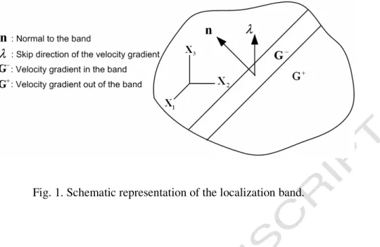
non-homogeneous straining mode becomes possible (i.e., the uniqueness of the solution of the rate equations is lost). This non-homogeneity is considered as a planar localization band, defined by its normal n (see Fig. 1). The velocity gradient inside and outside the band are respectively
ACCEPTED MANUSCRIPT
19
Fig. 1. Schematic representation of the localization band.
The nominal stress rate is related to the velocity gradient by the following constitutive law: :
=L G (54)
where L is an analytical tangent modulus that has to be expressed in terms of L and other ana fourth-order moduli induced by the large strain formalism. The continuity of the stress vector through the band of normal n is written as
⋅ =
n 0 (55)
where
[ ]
A =A+−A designates the jump in a quantity A across the chosen plane. Maxwell’s − compatibility condition for the velocity field states that a vector exists such that the jump inG reads
[ ]
G = ⊗n (56)Note that = 0 enforces a continuous velocity gradient field. Combining Eqs. (54)-(56), one obtains
(
n⋅ ⋅ ⋅L n)
= 0 (57)This is a typical eigenvalue problem and the existence of a nontrivial solution for (i.e., bifurcation condition ≠ 0 ) requires that the following determinant vanishes:
(
)
ACCEPTED MANUSCRIPT
20
This last equation gives a necessary condition for a localization band to appear (i.e., when the acoustic tensor becomes singular, thus corresponding also to the loss of ellipticity of the boundary value problem); it describes the strain localization criterion introduced by Rice (1976).
4.2. Tangent modulus for the ellipticity loss prediction
The application of the former localization criterion requires the calculation of the modulus
L . In a fixed frame, the hypo-elasticity law reads
(
)
: p
=C D D − (59)
where designates the Jaumann derivative of the effective Cauchy stress
= −W⋅ + ⋅W (60)
The stress rate can be thus expressed as (1 d) d
= − − +W⋅ − ⋅W (61)
The Cauchy stress and the nominal stress are related to each other by the classical relation
J = ⋅F (62)
where F is the deformation gradient and J =det(F) is its Jacobian. Thus,
(
)
1 ( )
J − tr
= F ⋅ D + − ⋅G (63)
In an updated Lagrangian formulation, F I and = J= ; Eq. (63) simplifies as: 1 ( )tr
= + D G − ⋅ (64)
and, replacing the Cauchy stress rate from Eq. (61) yields:
(
)
(1 d) p d ( )tr
= − C : D D− − − ⋅W+ D D − ⋅ (65)
All terms on the right-hand side of this above expression can be linearly expressed in terms of the velocity gradient G, in the following way:
(
)
(1−d) :C D D− p −d =Lana:G (66)
1
ACCEPTED MANUSCRIPT
21 2: ⋅ = D L G (68) 3: ⋅W L G = (69)where L is the analytical tangent modulus from Eqs. (24) and (33), while ana 1
L , L and 2 L 3
are fourth-order tensors that can be expressed, after some mathematical manipulations, as
1ijkl ij kl L =σ δ (70) 1 2ijkl 2 ik lj il kj L = δ σ +δ σ (71) 1 3ijkl 2 ik lj il jk L = σ δ σ δ− (72) and finally 1 2 3 ana =L +L L− −L L (73)
It is noteworthy that the resulting modulus L possesses no symmetry, due to the particular
forms of the three L terms. i
4.3. Numerical implementation of the localization criterion
The numerical detection of localization with Rice’s criterion can be considered as a mini-mization problem:
( )
( )
{
}
minimize with 1 det f f = = ⋅ ⋅ n n n n L n (74)In the case where min f
( )
n >0, there is no localization in the material point considered. Otherwise, ∃nloc / f( )
nloc =0, corresponding to the moment of the apparition of localization, where n represents all possible normal directions to the bands so formed. The applied algo-locrithm is composed of the following main steps:
1. Compute the tangent modulus L at the end of the loading increment. 2. Compute f
( )
n for different directions.3. Search the direction n , thereby giving the minimum of min f
( )
n .ACCEPTED MANUSCRIPT
22
o If .true. then nloc=n is the orientation of the first band and strain localiza-min
tion is reached.
o Otherwise, continue to 1 for the next loading increment.
5. Applications
In this section, the capability of the proposed approach to predict the FLDs, as well as the orientation of the shear bands, in monotonic and two-step sequential loading paths, is investi-gated. The study highlights the capability of the coupled model to predict different character-istics of the stress-strain relationship, especially its potential to simultaneously reproduce transient features of the hardening due to strain-path changes and the softening due to damage.
5.1. Validation of the constitutive model
Several direct and sequential loadings are considered for the investigation of the constitu-tive model and the validation of the computer implementation. The simulated tests correspond to typical in-plane sheet metal rheological tests, which are regularly used for the experimental and numerical assessment of FLDs using various models.
The materials used for the investigations are a dual phase high strength steel and a mild steel. The corresponding plastic anisotropy and hardening parameters (Hill’48 yield surface and Teodosiu-Hu hardening parameters) are listed in Table 1 and have been taken from Haddadi et al. (2006) and (3DS Report, 2001). The initial anisotropy is rather negligible for the dual phase steel (F, G, and H close to 0.5), while it is important for the mild steel. Plastic anisotropy is known to dramatically influence the forming limits and thus the use of the ani-sotropic Hill criterion is compulsory for the mild steel. Concerning hardening parameters, it is noteworthy that the latent part of the directional strength tensor, S , is deactivated for the L
dual phase steel, since C and r are set to zero. SL
In (Haddadi et al., 2006), the material parameters are also available for a simpler harden-ing model combinharden-ing the Armstrong-Frederick kinematic hardenharden-ing model, Eq. (14) without coupling to damage (i.e., d = , = , and = ), with the Swift isotropic hardening model: 0
(
0)
n p R
ACCEPTED MANUSCRIPT
23
where CR, and ε0 n are material parameters and ε p is the cumulated plastic strain. This clas-sical model will be used hereafter as a reference when useful; the corresponding parameters are also listed in Table 1.
One should note, however, that coupling with damage was not taken into account during the parameter identification of the elastic-plastic model. Parameter identification of damage models is a troublesome task and, to the knowledge of the authors, no attempt has been made to identify the parameters for the Teodosiu model coupled with damage. Moreover, the hard-ening parameters also depend on the parameter identification of the yield function, which also may influence considerably the FLD (Aretz, 2007). For the current work, a numerical study has been performed to address the impact of the damage parameters on the stress-strain curves and the FLDs. Consequently, a set of parameters has been chosen (see Table 2) that exhibits acceptable results, e.g., in terms of limit strains for simple tests. While one cannot consider the resulting set of parameters to correspond to the real materials under study, the use of the same set of damage parameters for both the Teodosiu model and the reference Armstrong-Frederick-Swift (AFS) model is believed to be consistent for the numerical comparison per-formed in the remainder of the paper.
ACCEPTED MANUSCRIPT
24
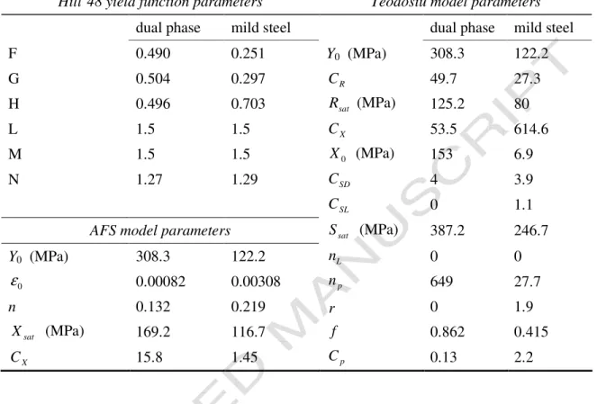
Table 1. Parameters of plastic anisotropy and hardening for the two materials analyzed in the paper, from Haddadi et al. (2006).
Hill’48 yield function parameters Teodosiu model parameters
dual phase mild steel dual phase mild steel
F 0.490 0.251 Y0 (MPa) 308.3 122.2 G 0.504 0.297 CR 49.7 27.3 H 0.496 0.703 Rsat (MPa) 125.2 80 L 1.5 1.5 CX 53.5 614.6 M 1.5 1.5 X0 (MPa) 153 6.9 N 1.27 1.29 CSD 4 3.9 SL C 0 1.1
AFS model parameters Ssat (MPa) 387.2 246.7
Y0 (MPa) 308.3 122.2 nL 0 0 0 ε 0.00082 0.00308 np 649 27.7 n 0.132 0.219 r 0 1.9 sat X (MPa) 169.2 116.7 f 0.862 0.415 X C 15.8 1.45 Cp 0.13 2.2
Table 2. Damage parameters used in the simulations.
Parameters e
i
Y (MPa) S s β
Values 0 2 1 5
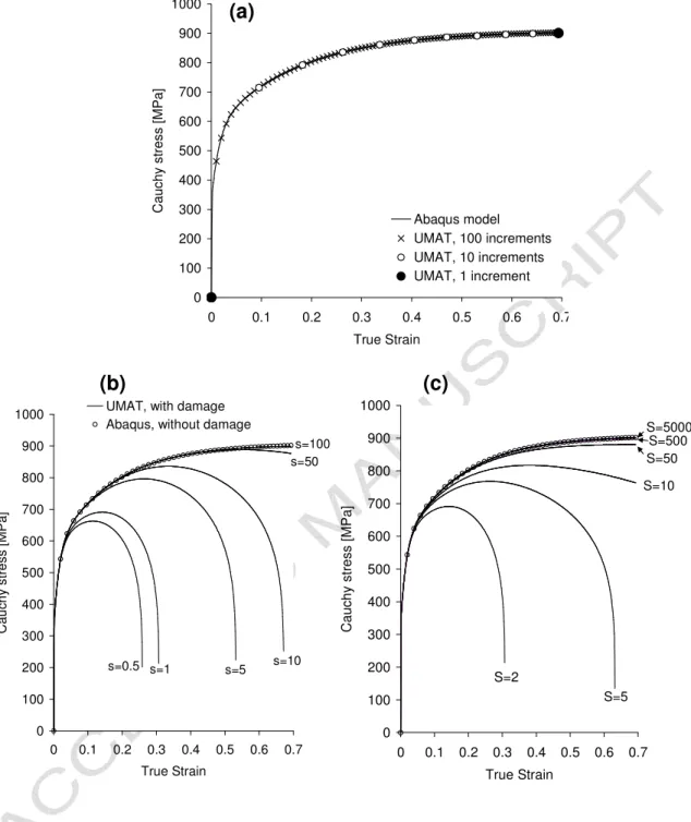
Fig. 2 illustrates the effectiveness of the implementation of the damage model in the FE code Abaqus and its numerical validation. Since the damage model adopted in this work is not available in Abaqus, the validation is performed with respect to the isotropic-kinematic hard-ening model (without damage), which is available in Abaqus. First, the same hardhard-ening model is obtained from the Teodosiu model by setting several parameters to zero and by deactivating the damage. As shown in Fig. 2a, the reference curve is obtained even when extremely large time increments are used. Next, the same reference curve is recovered by giving limit values
ACCEPTED MANUSCRIPT
25
to the damage parameters, when the damage law is activated. Through these simple simula-tions, the numerical implementation of the model appeared to be accurate and effective.
Fig. 3 shows the stress-strain predictions of several monotonic and two-step sequential tests for the mild steel. The effects of strain-path changes are clearly captured by the Teodosiu model for both reverse and orthogonal tests, as reported by Haddadi et al. (2006). On the other hand, the coupling with the damage model introduces softening behavior effects that were not available in the previous versions of the model. Other two-stage strain-path loadings will be further simulated in § 5.2 to analyze the effect of pre-strain on the FLD. Fig. 3b emphasizes the differences between the predictions of the two hardening models. As expected, the two models describe in a very different manner the transition zones after strain-path change; how-ever, the predictions of the remaining of the two-stage sequential tests are remarkably similar up to very large strains. While this figure illustrates well the consistency of the two models, it is noteworthy that the predictions of the shear test up to shear strains equal to 3 cannot be con-sidered realistic. In addition to the damage parameter identification, the choice of the Jaumann rate also becomes very questionable at such large strains. Indeed, although very popular in FE codes, this co-rotational description has been shown to exhibit some shortcomings when ki-nematic hardening is considered in the elastic-plastic constitutive modeling (Nagtegaal and De Jong, 1981; Lee et al., 1983). The main manifestation of this, which was first observed by Dienes (1979), is a spurious oscillatory shear stress response in simple shear test simulation when the strains become sufficiently large. This observation gave rise to extensive investiga-tions in the literature; some of which suggesting the use of alternative objective stress rates, while a more consistent treatment of this undesirable oscillation, pioneered by Dafalias (1985), seems to be the inclusion of the plastic spin as a variable in the constitutive modeling. How-ever, the evolution law of such a spin tensor is generally difficult to model; only microme-chanical physically motivated models give an explicit formula for the plastic spin, whereas in most phenomenological models it is assumed to vanish. In all the subsequent applications, however, the stress-strain curves should not go beyond the strain localization point as dis-cussed in Section 5.
ACCEPTED MANUSCRIPT
26 0 100 200 300 400 500 600 700 800 900 1000 0 0.1 0.2 0.3 0.4 0.5 0.6 0.7 True Strain C au ch y st re ss [M P a] Abaqus model UMAT, 100 increments UMAT, 10 increments UMAT, 1 increment(a)
(b)
(c)
0 100 200 300 400 500 600 700 800 900 1000 0 0.1 0.2 0.3 0.4 0.5 0.6 0.7 True Strain C au ch y st re ss [M P a]UMAT, with damage Abaqus, without damage
s=0.5 s=1 s=5 s=10 s=50 s=100 0 100 200 300 400 500 600 700 800 900 1000 0 0.1 0.2 0.3 0.4 0.5 0.6 0.7 True Strain C au ch y st re ss [M P a] S=2 S=5 S=10 S=500 S=50 S=5000
Fig. 2. Validation of the numerical implementation of the constitutive model; simulations of tensile tests for the DP material. (a) Validation of the elastic-plastic model with respect to the
Abaqus built-in model. (b), (c) Effect of the damage parameters s and S on the stress-strain curve.
ACCEPTED MANUSCRIPT
27 -300 -200 -100 0 100 200 300 400 500 -3 -2 -1 0 1 2 3Tensile true strain / shear strain
Te ns ile / sh ea r C au ch y st re ss [M P a] tensile test shear test orthogonal test (tensile + shear) Bauschinger tests (reverse shear) -200 -100 0 100 200 300 -0.1 0 0.1 0.2 0.3 -300 -200 -100 0 100 200 300 400 500 -3 -2 -1 0 1 2 3
Tensile true strain / shear strain
Te ns ile / sh ea r C au ch y st re ss [M P a] tensile test shear test orthogonal test (tensile + shear) Bauschinger tests (reverse shear) -200 -100 0 100 200 300 -0.1 0 0.1 0.2 0.3
AFS model – monotonic tests AFS model – reverse tests AFS model – orthogonal test Teodosiu model (sequential tests) Teodosiu model – monotonic tests Teodosiu model – reverse tests Teodosiu model – orthogonal test
a)
b)
Fig. 3. Different loading path simulations for the mild steel using the damage model coupled to: a) the Teodosiu model, b) the Armstrong-Frederick-Swift (AFS) model. Monotonous ten-sile and shear tests (dashed lines), reverse shear tests (thin line), 10% tenten-sile test followed by
a shear test (thick line). The (.)
11 Cauchy stress / logarithmic strain components are repre-sented for all situations but simple shear, when the shear Cauchy stress and shear engineering
strain components σ12 and γ12 =2 D dt12 are plotted instead. The zones of moderate strains are enlarged to emphasize the transition zone predictions after strain-path changes. All the
ACCEPTED MANUSCRIPT
28
5.2. Forming Limit Diagram prediction
As demonstrated by Rice (1976), the localization criterion considered here does not allow for the detection of strain localization in the case of an associative plasticity model with satu-rating stress-strain curves. This limitation is clearly illustrated in Fig. 4 (Top). In other terms, the introduction of a softening effect (by coupling the model with damage for instance) is re-quired for the activation of the criterion, as shown in Fig. 4 (Bottom).
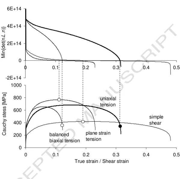
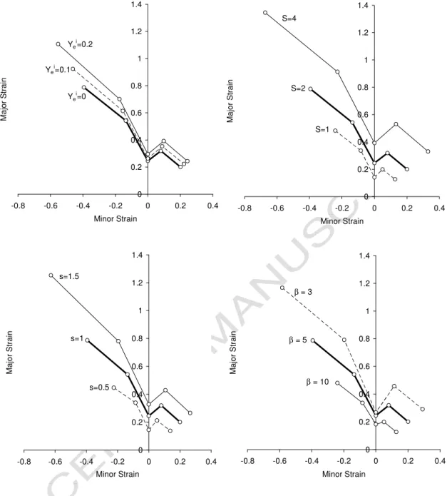
Fig. 5 illustrates the evolution of the localization criterion for different rheological tests as well as its respective predictions of limit strains. The strain state corresponding to the criterion activation is considered as the formability limit, and is plotted on the FLD. Fig. 6 shows the FLDs that correspond to various sets of damage parameters. As expected, delayed initiation of damage predicts higher formability limits. This figure clearly demonstrates the dramatic im-pact of the damage parameters on the formability prediction (see also Haddag et al. (2008)).
ACCEPTED MANUSCRIPT
29 0 0.2 0.4 0.6 0.8 1 0 200 400 600 800 1000 C au ch y st re ss [M P a] 0 0.2 0.4 0.6 0.8 1 0 1 2 3 4 5 x 10¹⁴ True strain m in [d et (n .L .n )] det(n.L.n)>0 0 0.05 0.1 0.15 0.2 0.25 0.3 0.35 0 200 400 600 800 C au ch y st re ss [M P a] True strain 0 0.05 0.1 0.15 0.2 0.25 0.3 0.35 0 5 10 15 20 x 1014 m in [d et (n .L .n )] det(n.L.n)=0Fig. 4. Detection of strain localization by means of Rice’s criterion in a uniaxial tensile test for the dual phase material without damage (Top) and with damage (Bottom).
ACCEPTED MANUSCRIPT
30 0 200 400 600 800 1000 0 0.1 0.2 0.3 0.4 0.5True strain / Shear stress
C au ch y st es s [M P a] -2E+14 0 2E+14 4E+14 6E+14 0 0.1 0.2 0.3 0.4 0.5 M in {d et (n .L .n )} balanced biaxial tension plane strain tension uniaxial tension simple shear
True strain / Shear strain
Fig. 5. Loading path simulations (bottom) and detection of strain localization by means of Rice’s criterion (top) for the dual phase steel.
ACCEPTED MANUSCRIPT
31 0 0.2 0.4 0.6 0.8 1 1.2 1.4 -0.8 -0.6 -0.4 -0.2 0 0.2 0.4 Minor Strain M aj or S tra in S=1 S=4 S=2 0 0.2 0.4 0.6 0.8 1 1.2 1.4 -0.8 -0.6 -0.4 -0.2 0 0.2 0.4 Minor Strain M aj or S tr ai n s=0.5 s=1.5 s=1 0 0.2 0.4 0.6 0.8 1 1.2 1.4 -0.8 -0.6 -0.4 -0.2 0 0.2 0.4 Minor Strain M aj or S tr ai n β = 3 β = 10 β = 5 0 0.2 0.4 0.6 0.8 1 1.2 1.4 -0.8 -0.6 -0.4 -0.2 0 0.2 0.4 Minor Strain M aj or S tr ai n Yei=0 Yei=0.1 Yei=0.2Fig. 6. FLDs for the mild steel predicted by means of the Rice criterion for different values of damage parameters. When not specified on the plots, the missing damage parameters take the values in Table 2. The thick curve on all the plots corresponds to the damage parameters
ACCEPTED MANUSCRIPT
32
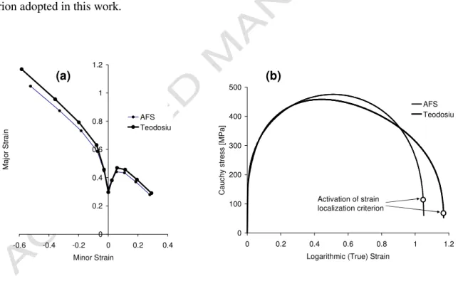
In the remainder of the paper, the same damage model and the parameters from Table 2 are used with either the Teodosiu or Armstrong-Frederick-Swift (AFS) hardening model. In order to illustrate the consistency of this choice, the tensile stress-strain curves for the mild steel and the FLDs corresponding to both situations are plotted in Fig. 7. The respective predictions of the two models are slightly different. One may note that, in the range of moderate strains where the hardening parameters are usually identified (up to 30…40% of tensile strain), the stress-strain curves almost coincide. Beyond the strain range that is typical for the identifica-tion of the hardening parameters, differences appear between the two predicidentifica-tions and, accord-ingly, the limit strains are somewhat different. As seen in Fig. 7a, the FLDs predicted by the two models are fairly close to each other, with the largest difference being observed for uniax-ial tension. Finally, the effect of a pre-strain on the FLD is shown in Fig. 8. The well-known “translation” of the FLD to the left in the case of uniaxial tensile pre-strain is observed, as well as the translation of the FLD to the right in the case of balanced biaxial pre-strain. Thus, the classical tendencies observed in experiments are well reproduced by the localization crite-rion adopted in this work.
0 0.2 0.4 0.6 0.8 1 1.2 -0.6 -0.4 -0.2 0 0.2 0.4 Minor Strain M aj or S tra in AFS Teodosiu 0 100 200 300 400 500 0 0.2 0.4 0.6 0.8 1 1.2 Logarithmic (True) Strain
C au ch y st re ss [M P a] AFS Teodosiu Activation of strain localization criterion (a) (b)
Fig. 7. Forming limit diagrams and tensile stress-strain curves for the mild steel predicted with the Teodosiu hardening model and the Armstrong-Frederick-Swift (AFS) model. The hardening parameters for both models are taken from (Haddadi et al., 2006), listed in Table 1,
ACCEPTED MANUSCRIPT
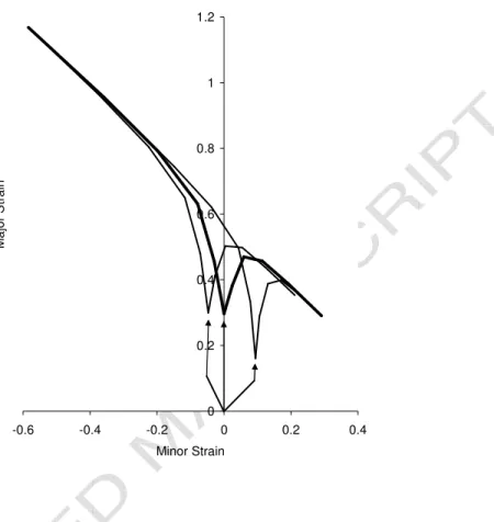
33 0 0.2 0.4 0.6 0.8 1 1.2 -0.6 -0.4 -0.2 0 0.2 0.4 Minor Strain M aj or S tra inFig. 8. Effect of 10% tensile and expansion pre-strains on the FLD predicted by means of Rice’s criterion (mild steel, Teodosiu model).
5.3. Orientation of the localization bands
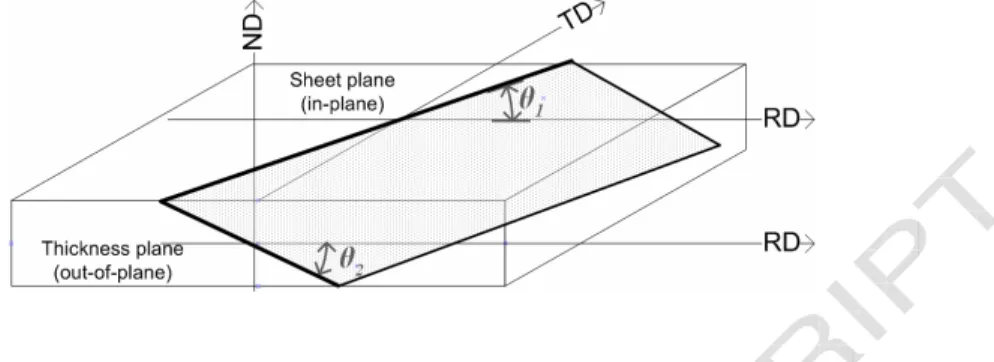
Rice’s localization criterion also provides the orientation of the localization band. This orientation can be defined by two angles, as shown in Fig. 9: the angle θ1 gives the inclina-tion of the band with respect to the rolling direcinclina-tion in the sheet plane (RD,TD), while the an-gle θ2 gives the inclination of the band with respect to the rolling direction in the thickness plane (RD,ND). For sheet materials, these two angles correspond to the in-plane orientation of the band, and a measure of its out-of-plane inclination. Most of the developments available in the literature assume a plane stress state and, moreover, do not take the out-of-plane inclina-tion into account (e.g. Lemaitre et al., 2000).
ACCEPTED MANUSCRIPT
34
Fig. 9. In-plane and out-of-plane orientation of the localization band of the sheet.
The orientation of the localization band is reported in Fig. 10 for different loading modes. The values of the in-plane angle for simple shear and uniaxial tension correspond to the clas-sically known experimental values as well as to those predicted with other models. For the plane strain tension, the result corresponds to the experimental observations, as well as to the prediction of the Marciniak-Kuczy ski model (for the in-plane orientation). On the contrary, calculations of plane strain tension using the Rice model, when the normal to the localization band is forced to lay in the sheet plane, predict an in-plane angle of about 75°…80° (depend-ing on the material model and parameters). Although the analysis is purely theoretical, the graphical representations clearly correspond to the experimental localization modes for the considered tests. The 3D analysis is not only useful for predicting the out-of-plane orientation of the band, but it is compulsory for a proper prediction of the in-plane orientation of the band and the corresponding limit strains. As shown in Fig. 10, the band is perpendicular to the sheet plane for simple shear and uniaxial tensile tests, while it is inclined at an angle of 45° to the sheet plane for plane strain tension. In the case of the equibiaxial tensile test, there is no privileged in-plane orientation for the band. As a final result, the effect of pre-strain on the band orientation has also been investigated during sequential rheological tests. After 5% and 10% of pre-strain in uniaxial tension or equibiaxial tension are applied, the band orientations are practically unchanged during the subsequent monotonic tests. Thus, no effect of the
pre-ACCEPTED MANUSCRIPT
35
strain on the orientation of the localization band has been noticed. However, the limit strains are strongly influenced. This aspect is further investigated hereafter.
Fig. 10. Sketches of the in-plane and out-of-plane orientation of the localization band of the sheet.
5.4. Influence of strain-path changes on the predicted FLDs
The dramatic impact of the strain path on the forming limits is well known. The concept of stress-based FLD (the σFLD) initiated by Arrieux et al. (1985) sought to provide an alterna-tive, strain-path independent way to address the sheet metal formability. However, the recent works of Yoshida and co-workers (Yoshida et al., 2007; Yoshida and Kuwabara, 2007; Yo-shida and Suzuki, 2008) provide experimental evidence and theoretical explanations of the strain-path dependency of the σFLD for particular cases of strain-path changes and, more generally, when the constitutive behavior of the material is strain-path dependent. It has also been shown (Gotoh, 1985; Kuroda and Tvergaard, 2000b) that the details of the loading pro-cedure during a strain-path change (with elastic unloading or not; with abrupt or continuous path change) strongly affect the results. Of equal importance, the constitutive model is known to affect the strain-path dependency of the FLD, at least when the Marciniak-Kuczy ski model is used (Hiwatashi et al., 1998; Yoshida and Suzuki, 2008). Since Rice’s criterion
re-ACCEPTED MANUSCRIPT
36
lies mainly on the constitutive tangent modulus to predict localization, its ability to capture the strain-path dependency on the FLD prediction is investigated here. Among several popular strain-path change possibilities (Nakazima et al., 1968), the combination of tensile or bal-anced biaxial pre-strains followed by plane strain tension has been shown to be insensitive to the details of the loading procedure adopted in the simulation (Kuroda and Tvergaard, 2000b). The mild steel is used for this investigation, as it exhibits complex strain-path-change tran-sient phenomena, and the predictions of the Teodosiu model are compared to those of the AFS model (both of which are coupled with damage).
The results of this investigation are summarized in Fig. 11. When the second loading mode is plane strain tension, the formability of the sheet material is dramatically reduced. As soon as the amount of pre-strain reaches a certain level, the strain localization appears imme-diately after the strain-path change. It is clear from Fig. 11 that this critical pre-strain level is smaller for the Teodosiu model than for the AFS model, whatever the pre-strain is tensile or biaxial. In order to understand the origin of these differences, the stress-strain curves corre-sponding to the two-path tests used to determine the FLDs are shown in Fig. 12 for both mod-els. The