Fast nonlinear solvers in solid mechanics
151
0
0
Texte intégral
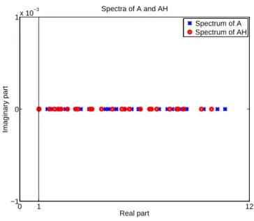
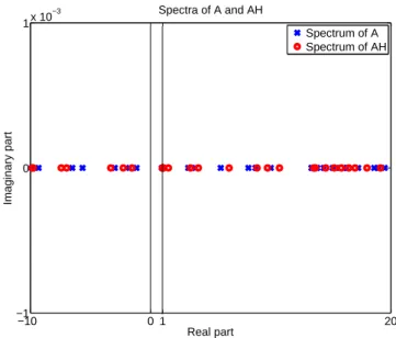
Figure
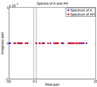
![Figure 2.1: Eigendistribution of A and AH: case of 1 ∈ [σ 1 , σ N ].](https://thumb-eu.123doks.com/thumbv2/123doknet/2106652.7836/60.892.289.651.664.973/figure-eigendistribution-ah-case-s-s-n.webp)
+7

Documents relatifs
