HAL Id: hal-00443763
https://hal.archives-ouvertes.fr/hal-00443763
Submitted on 4 Jan 2010
HAL is a multi-disciplinary open access archive for the deposit and dissemination of sci-entific research documents, whether they are pub-lished or not. The documents may come from teaching and research institutions in France or abroad, or from public or private research centers.
L’archive ouverte pluridisciplinaire HAL, est destinée au dépôt et à la diffusion de documents scientifiques de niveau recherche, publiés ou non, émanant des établissements d’enseignement et de recherche français ou étrangers, des laboratoires publics ou privés.
Fast characterization of radiation patterns of conformal
array antennas in the presence of excitation errors
Christine Letrou, Amir Boag, Amir Shlivinski
To cite this version:
Christine Letrou, Amir Boag, Amir Shlivinski. Fast characterization of radiation patterns of conformal array antennas in the presence of excitation errors. RADAR 2009 : International Radar Conference ”Surveillance for a safer world”, Oct 2009, Bordeaux, France. pp.1 - 5. �hal-00443763�
Fast Characterization of Radiation Patterns
of Conformal Array Antennas
in the Presence of Excitation Errors
Christine Letrou
Lab. SAMOVAR (UMR CNRS 5157) Institut TELECOM SudParis, Evry, France
Amir Shlivinski
Dept. of ECE, Ben-Gurion University Beer-Sheva 84105, Israel
Amir Boag
Dept. of Physical Electronics, Tel Aviv University Tel Aviv 69978, Israel
Abstract—A multilevel algorithm for the statistical
characterization of the radiation patterns of beam steered conformal arrays is presented. The algorithm can be used to obtain average complex field patterns and power patterns in the presence of random amplitude and phase excitation errors. The computational scheme is based on a hierarchical decomposition of the array into smaller sub-arrays. At the finest level of decomposition, the radiation patterns of single element arrays are computed or measured over a sparse grid of directions. The subsequent computational sequence comprises interpolations and aggregations of sub-array contributions repeated until obtaining the radiation pattern of the array. The proposed algorithm attains a computational complexity substantially lower than that of the direct computation and thus can be employed for Monte Carlo type statistical simulations.
Keywords-conformal array antennas; radiation patterns; calibration errors; multilevel decomposition
I. INTRODUCTION
Conformal array antennas offer well-known advantages over conventional planar arrays: aerodynamic shape, potentially greater effective aperture for a given platform, reduced weight. Conformal structural integrated antennas are thus of special interest for imaging radar systems mounted on the fuselage of an Unmanned Aerial Vehicle (UAV) or of an aircraft [1]. This new generation of radar imaging systems is based on multifunctional Synthetic Aperture Radars that aim at providing high resolution and long range imaging capabilities as well as highly sensitive ground moving target indication. Such radars make use of highly reconfigurable array antennas, with severe demands on beam direction precision, beam-width, and side-lobe levels, as required by high resolution algorithms. A large number of densely packed radiating elements is highly desirable for this type of antennas to increase the performance and achieve high space-time
resolution of the radiated fields over a wide angular sector of beam steering directions.
Evaluation of radiation patterns of such large arrays for a range of beam steering and observation directions poses a non-trivial computational challenge. Presence of excitation errors
due to random noise and imperfect calibration further
exacerbates the situation by requiring complex compensation techniques [2] and making the radiation patterns nondeterministic [3,4]. Some statistical properties of radiation patterns such as averages can be deduced from those of the excitation coefficients. However, probability density functions of radiation patterns can be obtained from those of the excitation coefficients, only at special points such as the main lobe peak and zeros, and, even this, using far reaching approximations [4]. Full statistical description can be obtained via Monte Carlo Type simulations at the cost of repeated evaluation of radiation patterns for various realizations of all random variables involved. Such brute-force approach comes at a substantial computational cost making a conventional radiation pattern evaluation for large conformal arrays impractical. In this paper, a multilevel array decomposition (MAD) algorithm [5,6] is introduced as a numerically efficient scheme for statistical characterization of the field and power radiation patterns (RPs) of arbitrary shaped arrays.
II. PROBLEM FORMULATION
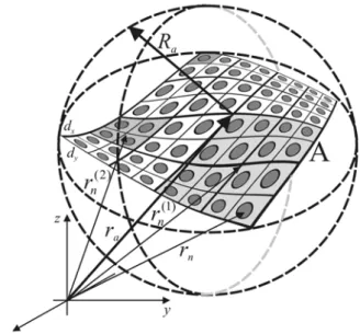
Consider an antenna array conformal to a surface S∈ R3
and comprising N radiating elements distributed over an arbitrary spatial lattice
{ }
rn nN=1∈S (see Fig. 1). We assume that the inter-element coupling is negligible. The array is circumscribed by a sphere of radius Ra centered at the array'sFigure 1. Example of a multilevel conformal array decomposition.
The elements are excited by incident currents
{
}
1
n N
j n n A eφ = . We assume that excitation amplitudes and phases are random variables, i.e., An =An(1+δAn) and φn =φ δφn+ n, where A n
and φ denote the mean values while n δAn and δφ denote n
zero mean statistically independent random variables. Here,
n
A describes the amplitude taper, and the phase
0
ˆ (n a)
n k
φ = − r ⋅ r −r is designed to steer the main beam to the
direction rˆ0 =(sinθ0cos ,sinϕ0 θ0sinϕ0,cos )θ0 defined by angles ( , )θ ϕ in the spherical coordinate system with the 0 0
origin at the array center ra.
The far field at an observation point r=rrˆ can be
expressed as E r r( ,ˆ0)≈U r r(ˆ ˆ,0)e−jkr/ 4πr , where we define the vector RP ˆ [ ( - )+ ] 0 1 ˆ ˆ ˆ ( ) n a n ( ) N j k n n n , A e ⋅ φ = =
∑
r r r U r r u r . (1)Here, u rn( )ˆ denotes the vector radiation pattern of the nth element produced by unit excitation current. The elemental radiation patterns
{
u rn( )ˆ}
nN=1 can be found by computation ormeasurement. For example, we have
[
]
ˆ ( ) ˆ ˆˆ ( ) ( ) jk n n jωμ n e d ⋅ − = −∫∫∫
1− ⋅ r r' r u r rr J r' r' where J rn( )denotes a physical or equivalent electric current distribution on the nth element’s due to unit excitation, see [5]. It must be noted that in typical non-planar arrays comprising identical radiating elements, the elements have different orientations and, consequently, their radiation patterns u rn( )ˆ are obtained by rotation of the elemental pattern with respect to the whole array. Hence pattern multiplication by an array factor, commonly used for planar arrays, is no longer valid. Instead, the field radiated by each element must be evaluated
separately for the observation directions ˆr defined in the
global coordinate system.
For given beam steering and observation directions, RP
0
ˆ ˆ
( , )
U r r behaves as a random variable due to the presence of
amplitude and phase errors, δAn and δφ . The statistical n
characterization of the stochastic RP can be effected along two paths described below. Though, the two approaches are markedly different, we will show that they can both greatly benefit from the use of the algorithm to be presented in the next section.
First, straightforward Monte Carlo type simulations can be enacted by performing array RP calculations for multiple realizations of the random errors. Towards evaluating the computational cost of this approach, we note that often the RP is of interest for all observation directions
ˆ (sin cos ,sin sin ,cos )= θ ϕ θ ϕ θ ∈ Ω
r and for all beam
steering directions rˆ0∈ Ω0 . Here, Ω and Ω0 denote the observation and steering direction domains of interest on the unit sphere. Since, the RP is an essentially bandlimited function with respect to the observation and steering angles, it may be represented by a finite set of samples. Angular
bandlimitness entails that for given Ω and Ω0, the RP is
calculated over grids of steering and observation directions
with numbers of points proportional to ( )2
a
kR , which (for
"uniformly populated'' arrays) is proportional to N . Thus, both Ω and Ω0 are sampled at ( )O N angular directions. The direct evaluation of U r r(ˆ ˆ,0) via (1) for all ˆr∈ Ω and rˆ0∈ Ω0
requires O N
( )
3 floating point operations. For a largenumber of elements this computational cost becomes prohibitively high. The situation is further exacerbated when, as stated above, the computations have to be repeated a large number of times, in order to obtain statistically reliable estimates of the RP parameters. Towards reducing the computational burden of such approach, in the next section we present the multi-level array decomposition method that accelerates the RP calculation.
As a computationally lighter alternative approach, we may attempt to evaluate the statistical parameters of the RP directly given the properties of the excitation errors. Thus assuming
for the phase error δφ Gaussian distributions with known n
standard deviation σ , we obtain the average RP φn
2/ 2 ˆ [ ( - )+ ] 0 1 ˆ ˆ ˆ ( ) n n a n ( ) N j k n n n , A e−σφ e ⋅ φ = =
∑
r r r U r r u r . (2)Note that the expectation of the random phase factor can be directly expressed as E e( jφn)=e ejφn −σϕ2/ 2 [7,8]. Comparing
(2) to (1), we note that the two expressions have the same
form except for replacing 2n/ 2
n n
A →A e−σφ and
n n
φ →φ . Thus,
average radiation pattern in (2) can be evaluated using the proposed fast algorithm developed for (1). When evaluating the effect of errors on the sidelobe levels, we are often interested in the average power pattern defined as
*
0 0
ˆ ˆ ˆ ˆ
[ ( ) ( )]
EU r r, ⋅U r r, . Directly multiplying (1) by its
conjugate, we obtain for the average power pattern
* * 2 0 0 0 0 ˆ ˆ ˆ ˆ ˆ ˆ ˆ ˆ ˆ [ ( ) ( )] ( ) ( ) U( ) EU r r, ⋅U r r, =U r r, ⋅U r r, +σ r . (3) where, 2 U
σ stands for the variance of the field RP that can be computed as 2 2 2 2 1 ˆ ˆ ( ) (1 n) | ( ) | n N U A n n n eσφ A σ σ − = =
∑
+ − r u r (4) with 2 n Aσ denoting the variance of δ . An
The average power pattern computation via (3) calls for the evaluation of the average RP already defined in (2). The
additional computation of 2
U
σ via (4) involves the elemental radiation patterns, which are slowly varying with respect to the beam steering and observation angles, since we assume that the radiating elements have dimensions comparable to the
wavelength. Thus, the evaluation of 2
U
σ can be performed on a very coarse grid of observation directions and subsequently interpolated and added to the rapidly varying terms on a fine angular grid. This makes the computational cost of obtaining
2
U
σ via (4) negligible in comparison with that of evaluating the vector field RP via (2). The latter computation will be accelerated by the algorithm described below.
III. MULTILEVEL ARRAY DECOMPOSITION ALGORITHM
The bandlimitedness property of the RPs, discussed in the previous section is employed here to formulate an efficient algorithm based on a multilevel array decomposition (MAD). The MAD algorithm starts by constructing a multi-level hierarchy of sub-arrays via a recursive decomposition of each array into M smaller arrays, Fig. 1. The smallest sub-array (highest level) consists of a single element, whose RP is a-priori known or computed over a sparse grid of observation directions. The lowest level sub-array is the entire array. Let
{
1, 2,}
G= …N denote the set of the array element indexes,
and ( )l n
G be the set of indexes corresponding to the nth
sub-array at decomposition level l, where l=0,1,…L ,
1, 2, l
n= …M , M is the number of sub-arrays at level l l
(M0 = at level 0, M at level 1, …) and L is the number of 1
decomposition levels. Furthermore, at a given level, each sub-array ("parent") gives rise to M sub-arrays ("children") of a
higher level, whose sets of indexes satisfy ( 1)l ( )l
m n n
G − = ∪ G
where P( )l ( )n = , i.e., the nth sub-array on level l is a child m
of the mth parent sub-array at level l-1. Next, assuming that
all sub-arrays at level l are similar in size, their corresponding
circumscribing sphere radii are ( )l / l/ 2
a an R =R M with (0) ( ) 1 L a a an R = N R =R , where ( )L an R is approximately the
single element circumscribing sphere, see Fig. 1. The nth
sub-array at level l is also characterized by a reference point ( )l
n
r
which is the center of its circumscribing sphere. Next, the array RP of Eq. (1) is rearranged to be evaluated by a recursive application of ( ) ( 1) ( ) ( 1) ( ) ˆ [ ( - )+ ] ( -1) ( ) 0 0 : ( ) ˆ ˆ ˆ ˆ ( ) ( ) nl ml nl ml l j k l l m n n P n m , , e ⋅ − φ −φ− = =
∑
r r r U r r U r r (5) where ( )L j n n nA en δφ = U u , (0) 1 U = U , and ( ) ( ) 0 ˆ ( - ) l l n k n a φ = − r ⋅ r r .The calculation begins with elemental patterns
( )L j n
n nA en
δφ =
U u at level l= and proceeds in the descending L
order l=L L, − …1, ,1 until the whole pattern (0)
1
U = U is
obtained. Note that for the mean RP computation the starting
point is ( )L 2n/ 2 n nA en φ σ − =
U u while the remainder of the
algorithm is unchanged.
A numerically efficient evaluation of RPs using Eq. (5) is achieved by noting that the numbers of angular points for the calculation of the RP of a sub-array at level l are dictated by
its electrical size ( )
n
l
a
kR . Thus, the observation and steering
grids of the lth level are sparser by a factor of M compared to
those of level l-1. An efficient transition from level l to level l-1, therefore, involves an interpolation and aggregation of
contributions from sparser to denser angular grids. For regular
arrays, a convenient hierarchy is set with M =4, i.e., the
increase in the number of grid points between the levels is achieved by doubling the number of points along each of the
angular dimensions, θ ϕ θ ϕ , by introducing a new , , ,0 0
direction between every two existing ones. Finally, for the calculation of the computational complexity, we shall be
interested in fast RP evaluation of U over 1≤D≤4 angular
dimensions (out of the four angular coordinates). Thus, calculating ( -1)l
m
U using Eq. (2) over the grid of level l-1
requires the evaluation of Ml sub-array contributions given
on the sparser lth grid. The resulting asymptotic complexity
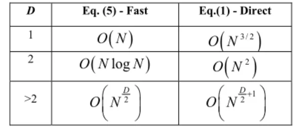
estimates for evaluating Eq. (2) for large array sizes are presented in Table I.
TABLE I. COMPUTATIONAL COMPLEXITY FOR VARIOUS PROBLEM DIMENSIONALITIES
The reduced complexity of the multilevel domain decomposition approach [5] and, in particular, the MAD algorithm [6] have been verified by extensive numerical studies. An example of array conformal to a conical surface will be presented in the following section.
D Eq. (5) - Fast Eq.(1) - Direct
1 O N
( )
O N(
3 / 2)
2 O N(
logN)
O N( )
2 >2 O N⎛ D2 ⎞ ⎜ ⎟ ⎝ ⎠ 1 2 D O N⎛⎜ + ⎞⎟ ⎝ ⎠IV. NUMERICAL EXAMPLE
As an example, we consider an array conformal to a conical surface, as shown in Fig. 2, based on the case study presented in [9], with array parameters in Tables I and II of this reference. The cone half angle is β π= / 6. The full array is composed of 256 linear arrays, aligned along the cone generatrix, equally spaced as a function of the azimuth angle
ϕ varying from 0 to 2π . The number of elements on each of
these linear arrays is 32. For a given beam position, 44 vertical linear arrays are active out of 256, and only active elements are shown in Fig. 2. The inter-element distance in "vertical" linear
arrays is 0.72λ , and the inter-element arc length along
horizontal ring arrays ranges from 0.51λ to 0.78λ , from the shortest ring array to the longest one.
The radiating elements are half wavelength dipoles with their axis along the generatrix of the cone. The cone is supposed to be perfectly reflecting, and the dipoles are placed
/ 4
λ above the cone surface. In the following, we use the
closed form expression of ideal half wavelength dipole pattern in front of a plane reflector for the fields radiated by individual elements, neglecting coupling effects.
The radius of the smallest sphere circumscribing the active
array is 19.35λ . With a number of decomposition levels
4
L= in the multilevel algorithm, the radius of the smallest
sphere circumscribing the smallest subdomains is 0.68λ . The
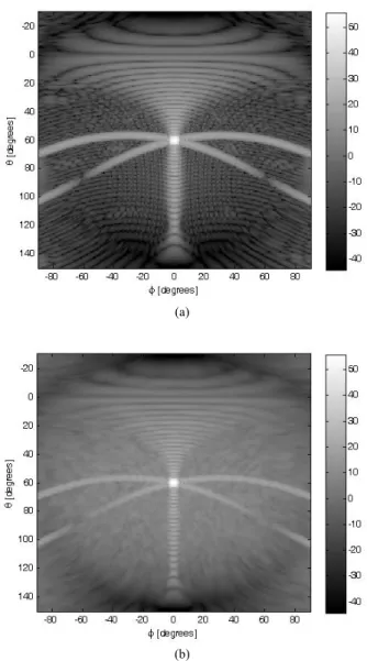
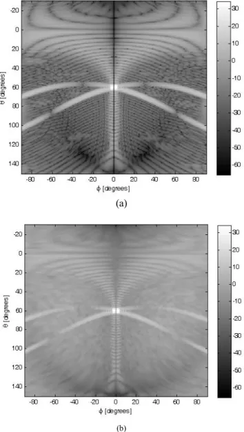
patterns of these subdomains are computed for 16( ) 24( )θ × ϕ directions. After successive interpolations and aggregations, we obtain the radiated patterns for 256( ) 384( )θ × ϕ directions. The 3D patterns presented in Figs. 3 and 4 are obtained with the symmetrically tapered excitation amplitudes given in [9, Table II], and with excitation phase designed to steer the main beam to the direction normal to the cone surface at the center of the array. Figs. 3a and 4a present (on a dB scale) co-polarized and cross-co-polarized patterns, respectively, for the array with perfect excitation coefficients. Corresponding patterns obtained by Monte Carlo simulations of arrays with random excitation coefficients are shown in Figs. 3b and 4b. We assume that the amplitude and phase variances for all of the excitation coefficients are the same, namely,
2 2
, An 0.01, n 0.01
n σ σφ
∀ = = . In this case, the power radiation
patterns have been averaged for 100 realizations of the random variables. By comparing the resulting patterns of the perfect array to those of the array with perturbed excitation coefficients, one can observe a significant increase in the sidelobe levels. On the other hand, as expected, the main lobe is hardly affected by the excitation errors.
Figure 2. Example of an array conformal to a conical surface.
(a)
(b)
Figure 3. Co-polarized radiation patterns of conical array (a) with perfect excitation and (b) with excitation errors.
(a)
(b)
Figure 4. Cross-polarized radiation patterns of conical array (a) with perfect excitation and (b) with excitation errors.
V. CONCLUSION
The statistical characterization of the radiation patterns of beam steering conformal antenna arrays using the multilevel array decomposition (MAD) approach has been proposed. The numerical efficacy of the MAD algorithm facilitates brute-force Monte Carlo type simulations or evaluation of statistical properties of RP based on those of the excitation coefficients. This algorithm is based on a multilevel hierarchical decomposition of the array into smaller sub-arrays. At the finest level of decomposition, the radiation patterns of single element arrays are computed over a sparse grid of directions. The algorithm comprises interpolations and aggregations of sub-array RP contributions that are repeated until obtaining the radiation pattern of the whole array. This algorithm attains a computational complexity which is substantially lower than that of the traditional direct computation.
REFERENCES
[1] J. H. G. Ender and A. R. Brenner, “PAMIR - a wideband phased array SAR/MTI system,” IEE Proc. Radar Sonar Navig., vol. 150, no. 3, pp. 165-172, June. 2003.
[2] H. Schippers et al., “Vibrating antennas and compensation techniques Research in NATO/RTO/SET 087/RTG 50”.
[3] R. J. Mailloux, Phased Array Antenna Handbook. Norwood, MA: Artech House, 1994, Ch. 7.
[4] A. K. Bhattacharyya, Phased Array Antennas. Hoboken, NJ: Wiley, 2006, Ch. 14.
[5] A. Boag and C. Letrou, “Multilevel fast physical optics algorithm for radiation from non-planar apertures,” IEEE Trans. Antennas Propagat., vol. 53, no. 6, pp. 2064-2072, June 2005.
[6] A. Shlivinski and A. Boag, “Fast evaluation of the radiation patterns of true time delay arrays with beam steering,” IEEE Trans. Antennas Propagat., vol 55, no. 12, pp. 3421-3432, Dec. 2007.
[7] R. E. Collin and F. J. Zucker, Antenna Theory, Part II. New York: McGraw-Hill, 1969.
[8] S. Seelig and Y. Rahmat-Samii, “Random surface error effects on offset cylindrical reflector antennas,” IEEE Trans. Antennas Propagat., vol 51, no. 6, pp. 1331-1337, June 2003.
[9] A. D. Munger, G. Vauchin, J. H. Provencher, B. R. Gladman, “Conical array studies,” IEEE Trans. Antennas Propagat., vol 22, no. 1, pp. 35-43, Jan. 1974.