HAL Id: hal-00433756
https://hal.archives-ouvertes.fr/hal-00433756
Submitted on 20 Nov 2009
HAL is a multi-disciplinary open access
archive for the deposit and dissemination of
sci-entific research documents, whether they are
pub-lished or not. The documents may come from
teaching and research institutions in France or
abroad, or from public or private research centers.
L’archive ouverte pluridisciplinaire HAL, est
destinée au dépôt et à la diffusion de documents
scientifiques de niveau recherche, publiés ou non,
émanant des établissements d’enseignement et de
recherche français ou étrangers, des laboratoires
publics ou privés.
Representations and Conditional Random Field
Wen Yang, Bill Triggs, Dengxin Dai, Gui-Song Xia
To cite this version:
Wen Yang, Bill Triggs, Dengxin Dai, Gui-Song Xia. Scene Segmentation via Low-dimensional Semantic
Representations and Conditional Random Field. EURASIP Journal on Advances in Signal Processing,
SpringerOpen, 2010, 2010, pp.196036. �10.1155/2010/196036�. �hal-00433756�
Scene Segmentation via Low-dimensional Semantic
Representation and Conditional Random Field
Wen Yang, Bill Triggs, Dengxin Dai, Gui-Song Xia
Abstract—In the past few years, significant progresses have
been made in scene segmentation and semantic labeling by integrating informative context information with random field models. However, many methods often suffer the computational challenges due to training of the random field models. In this work, we present a fast approach to obtain semantic scene segmentation with high precision, which captures the local, regional and global information of images. The approach works in three steps as follows: First, an intermediate space with low-dimension semantic “topic” representation for image patches is introduced, by relying on the supervised Probabilistic Latent Semantic Analysis. Secondly, a concatenated pattern is taken to combine the vectors of posterior topic probabilities on different feature channels and to incorporate them into a conditional random field model. Finally, a fast max-margin training method is employed to learn the thousands of parameters quickly and to avoid approximation of the partition function in maximum likelihood learning. The comparison experiments on four multi-class image segmentation databases show that our approach can achieve more precise segmentation results and work faster than that of the state-of-the-art approaches.
Index Terms—Scene segmentation, image labeling, logistic
regression, conditional random field.
I. INTRODUCTION
Semantic scene segmentation plays an increasingly impor-tant role in the fields of low-level, mid-level and high-level computer vision tasks for various and different goals. It jointly performs multi-class scene segmentation and object recogni-tion, also called image labeling, which requires to assigning every pixel by one of the predefined semantic classes, such as buildings, trees, water, car, and etc. After several decades of research on image segmentation, it is still a challenging problem due to the well-known “aperture problem” of local ambiguity. Recently, many innovative works are proposed to partially solve this problem by employing the informative contextual information, and this is often achieved by building a random field model over the images to encode the unary and pairwise probabilistic preferences.
Early labeling algorithms work at pixel level directly, but most recently works operate at higher-level (often superpixels or patches, which are small groups of similar pixels) due to the efficiency and consistency. In this work, we prefer to chose the patch-based representation: one for the convenience of
W. Yang and D.X. Dai are with the Signal Processing Lab, School of Electronics Information, Wuhan University, Wuhan, 430079 China e-mail: [email protected]; [email protected].
B. Triggs is with Laboratoire Jean Kuntzmann, B.P. 53, 38041 Grenoble Cedex 9, France e-mail: [email protected]
G.-S. Xia is with CNRS LTCI, Institut Telecom, TELECOM ParisTech, 46 rue Barrault, 75634, Paris Cedex-13, France, e-mail: [email protected]
utilizing considerable local descriptors, the other is for the ease of inference on the Conditional Random Field (CRF) model.
Our goal in this work is to combine multiple theoretical ideas in order to obtain a easy-to-use high performance seg-mentation method. In a nutshell, given an image the proposed approach works as follows: First, we use a logistic regression classifier (LRC) to form our low-dimensional feature represen-tation for each image patch. Then, we build a CRF model to integrate the local, regional and global information. Finally, we efficiently train and test the CRF model, by using a fast max-margin solver and energy optimization algorithm. We evaluate our method on two partially labeled data sets: the 9-class and 21-class MSRC image databases (Criminisi 2004 [1]) as well as two fully labeled datasets: 7-class Corel and Sowerby databases (He et al. 2004 [2]).
The main contributions of this paper are as follows:
∙ Propose a low dimensional semantic “topic” representa-tion for each image patch, and use a concatenated mode to combine different modalities for characterizing the patch;
∙ Introduce an improved global object labels distribution to indicate the spatial context, and use a Markov Random Field (MRF) neighborhood system to incorporate the re-gional information which implicitly attempt ot model the relative location information of different object classes;
∙ Use FastPD optimization [3] and cutting plane algorithm via “1-slack” formulation to efficiently and exactly solve the maximum margin learning of parameters for our CRF model [4], [5], [6].
In the rest of this paper, we first review the previous and related works in Section II. We then describe how to extract and represent the local and context information in Section III, and propose our two-stage segmentation model and learning method in Section IV. In Section V, we demonstrate the ex-perimental results and present several interesting discussions. The conclusions and future work are given in Section VI.
II. PREVIOUS AND RELATED WORK
This section briefly summarizes different methods that have been explored for scene segmentation and semantical labeling. He et al. [2] proposed a multiscale CRF to combine the local, regional and global label features, however, it needs inefficient stochastic sampling for learning the model and inferencing the labels, and further research in [7] presented a discriminative image segmentation framework that integrates bottom-up and top-down cues to include a considerably wider range of object classes than earlier methods. Kumar et al. [8] presented a two-layer CRF to encode the long-range and
short-range interactions. The boosted random fields [9] used Boosting to learn the graph structure and local evidence of a conditional random field. Shotton et al. [10] described a discriminative model of object classes by incorporating texture, layout, and context information efficiently. Verbeek et al. [11] learned a CRF from partially labeled data and incorporated top-down aggregated features to improve the segmentations. Yang et al. [12] implemented the multiple class object-based segmentation by using the appearance and bag of keypoints models integrated over mean-shift patches. Schroff et al. [13] incorporated globally learnt class models into a random forest classifier with multiple features, and imposed spatial smoothing via a CRF model for a further increase in performance. In [14], the authors presented a CRF that models local information and global information, and demonstrates high performance in image labeling of two small fully labeled data sets.
Many researches of image labeling focus on the utilization of high-level semantic representation and informative context information. Recent work by Rabinovich et al. [15] incorpo-rates semantic context by constructing a conditional Markov random field over image regions that encodes co-occurrence preferences over pairwise classes. In [16], the authors com-bined the advantages of Probabilistic Latent Semantic Analysis (PLSA) model and spatial random fields to improve the overall accuracy. Cao et al. [17] used Latent Dirichlet Allocation at the region level to perform segmentation and classification and enforce the pixels within a homogeneous region to share the same latent topic. The latent topic random field model [18] learned a novel context representation in the joint label and image space by capturing co-occurring patterns within and between image features and object labels, and in [19], the au-thors further explored a hybrid model framework for utilizing partially labeled data that integrates a generative topic model for image appearance with discriminative label prediction. Csurka et al. [20] proposed a simple framework to semantic segmentation which uses the Fisher kernel to derive high-level descriptors for computing the patch level class-relevance and use classification at the image level to take into account the objects context. Tu [21] introduced an auto-context model to improve the scene parsing performance significantly by taking effective context information. However, the training time takes a few days. Shotten et al. [22] presented a semantic texton forests method to infer the distribution over categories at each pixel, and use an inferred image-level prior to obtain state of the art performance, which needs a trade-off between the memory usage and the training time.
Earlier works mostly consider simple object location in-formation, such as the absolute location of objects in the scene. In [23], the authors applied the objects relative location relations to capture the spatial context, such as above, below, inside and around. Gould et al. [24] proposed a novel image-dependent relative location feature which can model compli-cated spatial relationships, and achieved results above state of the art through a two-step classifier with this relative location preference.
Most similar to us is the work of Verbeek and Triggs [11] which build a CRF segmentation model to capture the global
context of image as well as the local information. However, there are several important differences with respect to our work. First, we add a new feature channel of texton based on the feature extraction scheme of [11] and replace the absolute position information in [11] with a more informative position feature which represents the global spatial configuration of labels. Second, unlike [11], which uses a histogram of visual words representation for each patch, we represent each patch as concatenated vectors of posterior “topic” probabilities, which helps to remove the redundancy that maybe present in the basic “bag of features” model. Moreover, a lower dimensional latent topic representation speeds up computation. Third, we incorporate the regional information into our CRF model through a MRF neighborhood system, which implicitly includes the relative location information of different object classes. We finally employ the recently proposed FastPD [3] algorithm and cutting plane algorithm [6] to efficiently imple-ment the maximum margin learning of parameters exactly for our CRF model, and demonstrate significant improvements in accuracy, speed and applicability.
III. MODELING LOCAL AND CONTEXT INFORMATION
In this section, we first describe the extraction of visual features in more detail. Then, we present a low-dimensional semantic representation using supervised PLSA. Next, we in-troduce our improved object labels spatial layout information. We finally show how to obtain the regional and global context information.
A. Local Patch Descriptors
Many different approaches to patch description have been proposed in the literature, which emphasize different image properties such as pixel intensities, color, texture, and edges. Here, we compute three types of features for each patch: SIFT [25], color and textons, which is similar to that of Verbeek and Triggs [11], except that we use a new texton channel to replace the absolute position information. Textons are computed based on an efficient implementation of comput-ing gabor features named “simple Gabor feature space” [26] which leads to a remarkable computational enhancements. Simple Gabor feature space is also an efficient structure for representing and detecting small and simple image patches. To further enhance the robustness of color descriptors under photometric and geometrical changes for different scenes, we use a consolidated representation for each patch through concatenating the normalized hue descriptor and opponent angle [27]. The former is robust to scenes with saturated colors, while the latter is suitable for scenes with less saturated colors.
B. Low-dimensional semantic representation
Bag-of-features model has recently shown very good per-formance for image categorization which was originated from “bag of words” model in natural language processing (NLP) or information retrieval. We can also apply this representation on patch representation and classification. Each patch is thus
encoded by a binary vector with a single bit set corresponding to the observed visual word. However, it will lead to the big dimensions of features. For example, if we quantize SIFT, color and texton descriptors using visual codebooks of 1000 centers by kmeans, and use the concatenated binary indicator vector of its three visual words as in [11], we will obtain a 3000-dimension features for each patch, which results in a very high computational cost in later CRF model training.
Another impressive model related to bag-of-features strat-egy is the latent topic model, such as the probabilistic Latent Semantic Analysis [28] or its bayesian form, the Latent Dirich-let Allocation (LDA) [29]. They consider visual words as gen-erated from latent aspects (or topics) and expresses images as combinations of specific distributions of topics, which partially meet the desire for low dimensional image representations. In [30], Quelhas et al. use PLSA, to generate the compact representation. They argue that PLSA has the dual ability to generate a robust, low dimensional scene representation, and to automatically capture meaningful scene aspects or themes. PLSA is also used by Bosch et al. in image classification [31]. Li et al. [32] propose two variations of LDA to generate the intermediate theme representation to learn and recognize natural scene categories, and report satisfactory categorization performances on a large set of complex scenes. Rasiwasia et al. [33] introduce a low-dimensional semantic “theme” image representation which correlates well with human scene understanding, and achieve performance close to the state of the art methods on scene categorization with much smaller training complexity. There are also some more complicated topic models, such as Harmonium model based on undirected graphical models [34], Pachinko Allocation Model based on directed acyclic graph [35], and their variants. We prefer to use PLSA for its efficiency computation and comparable accuracy in practice [16].
In standard PLSA, each topic 𝑡 is characterized by its dis-tribution𝑃 (𝑤∣𝑡) over the 𝑊 words of the dictionary, and each document 𝑑 is characterized by its vector of mixing weights
𝑃 (𝑡∣𝑑) over topics. Then the probability model 𝑃 (𝑤∣𝑑) is
defined by the mixture,
𝑃 (𝑤∣𝑑) =∑𝑇
𝑡=1
𝑃 (𝑤∣𝑡)𝑃 (𝑡∣𝑑) (1)
Generally speaking, both 𝑃 (𝑤∣𝑡) and 𝑃 (𝑡∣𝑑) are estimated by EM algorithm, However, here we assume 𝑃 (𝑤∣𝑡) is ob-tained by simply count the occurrence of words and topics in the training images. So the EM reduces to use in the inference stage, which is also called “fold-in” techniques [16]. It is used to estimate the topic probabilities for new test images after the likelihoods of words given topics are learned on the training set. In this case, the semantic topics are explicitly defined, PLSA can be thought of as a data-driven technique that use the fact that a given group of words or observations all originated from the same document or image to infer a context specific prior via statistical inversion [36].
By considering image patches as distributions of topics, we can use the topic distribution as the patch feature rep-resentation. The number of object classes defines the
dimen-sionality of the intermediate topic space.Each topic induces a probability density on the space of low-level features, and each patch is represented as the vector of posterior topic probabilities. In particular, we firstly use a supervised PLSA classifier to predict the topic distribution of each patch relates to the predefined object semantics, and then we obtain the concatenated probability outputs of the three individual PLSA classifier for SIFT, Color and Texton descriptor (To cope with the huge possible distinct output index combinations, we also make the usual Na¨ıve Bayes assumption that the three feature channels are conditionally independent given the underlying class label). Now, we can reduce the dimension of 3000-dimension patch representation to three times of topics number (for MSRC-9 and MSRC-21 class dataset, they are only 27 and 63 dimensions, respectively), Further, we can use a multi-modal PLSA in [11] to obtain a more compressed representation. For the multi-modal PLSA model, the formulation assume the three modalities are independent given the topic,
𝑃 (𝑤∣𝑑) =∑𝑇
𝑡=1
𝑃 (𝑤𝑠𝑖𝑓𝑡∣𝑡)𝑃 (𝑤𝑐𝑜𝑙𝑜𝑟∣𝑡)𝑃 (𝑤𝑔𝑎𝑏𝑜𝑟∣𝑡)𝑃 (𝑡∣𝑑) (2)
By using multi-modal PLSA, we can further reduce the dimension of features on each patch to only the number of topics.
C. Spatial layout distributions of scene categories
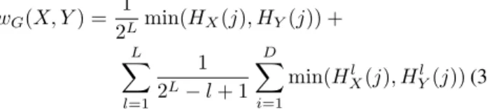
We have described a patch by integrating the color, structure and texture information. However, we do not include spatial position information of patches. There are different ways to involve the spatial layout information, such as the absolutely position information in [11], the position features are obtained by quantizing using a uniform𝑚×𝑚 grid cells superimposed over the image, the index of the cell in which the patch falls as its position features. [14] proposed a scene similarity weighted global spatial labels information, the idea behind which is that similar scenes tend to share a similar configuration of category distributions. It computes the scene similarities using a global color features based on Euclidean distance criteria and shows good performance and recognizes the scene appearances by incorporating the global image features and the spatial layout of labels. Inspired by the work of [14], we adopt a modified version of global location information by using a spatial pyramid matching method to obtain the scene similar-ity. In principle, spatial pyramid matching (SPM) scheme is possible to integrate geometric information directly into the original pyramid matching framework [37] by treating image coordinates as two extra dimensions in the feature space [38]. Firstly, we apply the spatial pyramid matching method to compute the scene similarities using the obtained sift and color descriptors on the regular grid from each image. Let
𝑋 and 𝑌 be two sets of vectors in a d-dimensional feature
space, 𝑙 denotes one resolution from a sequence of grids at resolutions0, . . . , 𝐿, 𝐻𝑋𝑙 and𝐻𝑌𝑙 are the histogram of𝑋 and
𝑌 at this resolution, respectively. 𝐻𝑙
𝑋(𝑗) and 𝐻𝑌𝑙(𝑗) denote
of the grid, so the final similarity of two different scenes can be computed as follows, 𝑤𝐺(𝑋, 𝑌 ) =21𝐿min(𝐻𝑋(𝑗), 𝐻𝑌(𝑗)) + 𝐿 ∑ 𝑙=1 1 2𝐿− 𝑙 + 1 𝐷 ∑ 𝑖=1 min(𝐻𝑙 𝑋(𝑗), 𝐻𝑌𝑙(𝑗)) (3)
Then, the pixelwise spatial label distribution is computed using a weighted combination of the training data [9]:
𝑃 (𝑙𝑝= 𝑐∣𝑓𝐺) = 𝐾
∑
𝑘=1
𝑤𝐺(𝑌, 𝑌𝑘)𝐵𝑘𝑐(𝑝) (4)
Here, 𝐵𝑡𝑐(𝑝) is the hand-labeled data of a training image
𝑌𝑘. If the hand-labeled category at a pixel 𝑝 is category 𝑐,
𝐵𝑐
𝑘(𝑝) indicates “1”; otherwise, it indicates “0”. 𝑤𝐺(𝑌, 𝑌𝑘) is
obtained by spatial pyramid matching as a weight function that reflects the scene similarity. In [14], the authors considered the contributions of all the training images to the pixelwise distribution, which is suitable for the small dataset, such as sowerby and corel dataset they used. However, for the more comprehensive and complex datasets, such as MSRC-9 class and MSRC-21 class dataset, using all the training data will leads to high computational effort and also decrease the performance slightly. Therefore, we employ the KNN idea to compute the pixelwise spatial label distribution. In more detail, it selects the 𝐾 most similar images to the new test image within the training database (using the similarity metric based on SPM above).Then it predicts the pixelwise spatial label distribution of the test image by weighting the category label distribution within the𝐾 similarest training images.
Finally, the patchwise spatial distribution is obtained as the average distribution of 𝑃 (𝑙𝑝∣𝑓𝐺) within patch 𝑖
𝑃 (𝑙𝑖∣𝑓𝐺) = ∣𝑆𝑃1 𝑖∣
∑
p∈SPi
𝑃 (𝑙𝑝∣𝑓𝐺) (5)
In our case,∣𝑆𝑃𝑖∣ is a constant which equals to the size of the patch.
D. Regional and Global Information
To describe the relationship of the central patch and its neighbours, we use the MRF neighbour system as Fig. 1, which shows in turn the first order, the second order and the whole fifth neighborhood system. The shape of a neighbor set may be regarded as the hull enclosing all the sites in the set [39].The context information for a given neighborhood is computed by taking the topic distribution of each patch and concatenating them together directly, resulting in a high-dimensional feature vector depends on the number of topics. For example, considering a 5-order neighbours system for MSRC-9 data, we will get a 225 dimensions feature vector for each patch. The neighbour system features implicitly includes relative position information of different objects.
For taking the image-level context into account, we also use the averaged topic probability on the whole image as
Fig. 1: The first, second and fifth-order MRF neighborhood system
the global aggregated features [11]. Intuitively, regional and global contexts should be complementary, as they capture different types of dependencies. The regional context partially includes the relative position information of different topics, and can yield spatially varying priors. The image-level context can capture the dependence of all the patches within the image on the same underlying scene, but it can only produce priors that are constant over the entire image.
IV. SCENE SEGMENTATION BASED ONCRFMODEL
Our labeling framework is a two-stage method. Fig.2 shows the flowchat of labeling process. At the first stage, LRC is trained to predict the posterior probability vectors of each patch. Essentially, it firstly uses the supervised PLSA to com-pute the topics probabilities of each patch with respect to the three different feature channels-SIFT, color and gabor. Then, a LRC is applied to classify each patch by concatenating the three predicted topic distribution by PLSA and the predicted spatial labels distribution as features. At the second stage, we use a CRF to learn correlations between neighboring output labels helps resolve ambiguities, where the input to the CRF is the combination of local, regional and global features.
The first stage method treats the labeling problem as un-structured, we can also employ other standard discriminative classifiers, such as SVM, adaboost or random forest, and we use logistic regression for its simplicity and higher computa-tional speed. At the second stage we apply a CRF classifier to include the spatial couplings (pairwise CRF potentials) and we refer it as LRC/CRF. Naturally, we can use LRC again, which also gives a competitive performance with lower computation cost, and we refer it as LRC/LRC.
Fig. 2: Pipeline of our two-stage semantic scene segmentation method
A. The Regularized Logistic Regression
Logistic regression is a simple yet effective classification algorithm which naturally fits within the probabilistic frame-work of a CRF model. Since the logistic model decomposes over individual patches, training and evaluation are both very
efficient. Given feature data x and weights (w, b), the prob-ability model of logistic regression classifier is
𝑃 (y∣x, w) =1 + exp(−y(w1 𝑇x + b)) (6) where y is the class label. Moreover, to obtain good generalization abilities, a regularization term w𝑇w/2 can be added. So the regularized logistic regression [40] is as follows,
min w 𝑓(w) ≡ 1 2w𝑇w + 𝐶 𝑛 ∑ 𝑖=0 log(1 + exp(−y𝑖w𝑇x𝑖)) (7)
where 𝐶 > 0 is the balanced parameter for the two terms in the above equation. In [40], the authors apply a trust region Newton method to maximize the log-likelihood of the logistic regression model, and show that it is faster than the commonly used quasi Newton approach and yields excellent performances.
B. CRF model
Typically, a logistic regression model is not sufficiently expressive and some explicit pairwise dependence is required. Indeed, most recent works on probabilistic image segmen-tation use conditional random fields to encode conditional dependencies between neighboring pixels and superpixels. The CRF formulation allows a smoothness preference to be incorporated into the model. Furthermore, pairwise features also encapsulate local relationships between regions.
Standard CRF has the following distribution form [41]:
𝑃 (𝑋∣𝑌 ) = 𝑍1𝑒𝑥𝑝 ⎧ ⎨ ⎩− ⎡ ⎣∑ 𝑖∈𝒱 𝜙𝑖(𝑓𝑖) + ∑ (𝑖,𝑗)∈ℰ 𝜓𝑖𝑗(𝑥𝑖, 𝑥𝑗) ⎤ ⎦ ⎫ ⎬ ⎭ (8) where𝑌 is an input data, 𝑋 is the corresponding labels, 𝑍 is the partition function,𝒱 is a set of nodes of the image, and ℰ is the pairs of adjacent nodes.𝜙(⋅) is the unary potential term, and 𝜓(⋅) is the pairwise term. In practice, log-linear models (e.g., MRF and CRF) form the most common model family for labeling problems. Generally, the energy function of these models is a linear combination of a set of feature functions.In this paper we label images at the level of small patches, using CRF to incorporate the purely local (single patch) feature functions, the regional neighbors of the current patch and more global “context capturing” feature functions that depend on aggregates of observations over the whole image. Our energy formulation can be written as follows,
𝐸(𝑋, 𝑌 ) =∑ 𝑖∈𝒱 𝑊 ∑ 𝑤=1 ( 𝛼𝑤𝑙𝑦𝑙𝑜𝑐𝑖𝑤 + 𝑁 ∑ 𝑛=1 𝛽𝑛𝑤𝑙𝑦𝑟𝑒𝑔𝑖𝑤𝑛+ 𝛾𝑤𝑙𝑦𝑤𝑔𝑙𝑜 ) + ∑ (𝑖,𝑗)∈ℰ 𝜓𝑖𝑗(𝑥𝑖, 𝑥𝑗) (9)
Where 𝑦𝑖 denotes a W-dimensional feature vector, 𝑥𝑖 ∈
{1, . . . , 𝑙, . . . , 𝐿} denotes the label of node 𝑖. (𝑖, 𝑗) denotes
the set of all adjacent (4-neighbor) pairs of patches 𝑖, 𝑗. The
parameters𝛼𝑤𝑙 ,𝛽𝑛𝑤𝑙 and 𝛾𝑤𝑙 are𝑊 × 𝐿,𝑁 × 𝑊 × 𝐿 and
𝑊 ×𝐿 matrices of coefficients to be learned, respectively. For
the pairwise potential, we choose a simple Potts model which has a clique potential for any pair of neighboring pixels𝑖 and
𝑗 given by
𝜓𝑖𝑗(𝑥𝑖, 𝑥𝑗) = 𝜎[𝑥𝑖∕= 𝑥𝑗] (10) Where[⋅] is one if its argument is true and zero otherwise. 𝜎 is the parameter to be learnt. The results of [11] indicate that the simple Potts model gives the best performance in sevral forms of pairwise potential.
C. Parameters estimation of CRF model
Currently, the most widely used learning algorithms in-clude cross-validation and some partition function approxima-tions [4]. Here we will investigate two classes of CRF learn-ing methods: maximum likelihood method and max margin method.
CRF model defines a conditional distribution of output label given the input. Applying the Maximum Likelihood principle to the conditional distribution, we obtain the conditional maximum likelihood (CML) criterion. The Maximum likeli-hood learning of discriminative models may suffer from the overfitting and difficult model selection problems. Here we use a stochastic gradient descent method [42] to provide a faster convergence rate for maximizing the log likelihood. The sum-product loopy belief propagation method is used to handle the partition function (using the Bethe free energy approximation for partially labeled images described in paper [11]).
Max margin learning method employs the energy function of CRF model as a discriminative function. The advan-tage of the margin-based approach is that the learning can be formulated as a quadratic programming problem. Also, we can introduce the kernel trick to create a set of more powerful feature functions. However, this approach results in exponentially many constraints in the optimization. The Maximum Margin Markov Network(𝑀3𝑁) method combines maximum-margin and output correlation constraints into a single quadratic programming optimization problem, and using dual extragradient method to accelerate the training speed [43]. Szummer [4]presented an efficient algorithm to train ran-dom field model (MRF and CRF) for images based on the structured support vector machine (SVMstruct) framework of Tsochantaridis et al. [44] and the maximum-margin network learning of Taskar et al. [45] [46]. It start from a standard large-margin framework, and then leverage graph cut [47] to perform inference to efficiently learn parameters of random fields which are not tractable to train exactly using maximum likelihood training.
Following the idea of [4], we use a 1-slack cutting-plane training method instead of the n-slack method [4] used. Joachims [6] pointed out the 1-slack algorithm is substantially faster than n-slack algorithm on all problems, for multi-class classification and HMM by several orders of magnitude. In addition, we will apply the FastPD algorithm [3] instead of the alpha-expansion graph cut in [47] as the final energy op-timization method. The FASTPD algorithm generalizes prior
state-of-the-art methods such as alpha-expansion, while it can also be used for efficiently minimizing NP-hard problems with complex pair-wise potential functions. It can be proved that Fast-PD is as powerful as alpha-expansion, in the sense that it computes exactly the same solution, but with a substantial speedup- of a magnitude ten - over existing techniques [48]. Moreover, contrary to alpha-expansion, the derived algorithms generate solutions with guaranteed optimality properties for a much wider class of problems, e.g. even for MRF with non-metric potentials, they are capable of providing per-instance suboptimality bounds in all occasions, including discrete Markov Random Field with an arbitrary potential function.
For the convenience of description, we rewrite the pseu-docode for the max-margin learning algorithm [4], [6] as follows,
TABLE I: Pseudocode for 1-slack margin scaling learning algorithm
Input:
-input labeling pairs(y(𝑛), x(𝑛)) training set(𝑛 = 1, . . . , 𝑁) -empty set of competing low energy labelings:𝑆 = ∅ -initial parameters:w = w0, the penalized parameter𝐶,
and the desired precision𝜀
Repeat untilw is unchanged
Loop over all training samplesn
Step1: Find the MAP labeling of sample𝑛
x∗← 𝑎𝑟𝑔𝑚𝑖𝑛𝐸x(y𝑛, x; w)
Step2:Ifx∗∕= x(𝑛), addx∗to the constraint set
𝑆∗← {𝑆(𝑛)∪ x∗}
Step3: Update the parametersw to ensure the ground truth
has the lowest energy
minw,𝜉≥012 ∥ w ∥2+𝐶𝜉 s.t.∀x ∈ 𝑆𝑛∀𝑛 1 𝑛[𝐸x(y(𝑛), x; w) − 𝐸x(y(𝑛), x(𝑛); w)] ≥𝑛1 ∑𝑁 𝑛=1△(x(𝑛), x) − 𝜉 V. EXPERIMENTALRESULTS
In this section we present our experimental results, and compare the performance of our method to recently published state-of-the-art results on four datasets: the 21-class and 9 class MSRC datasets of [1]; and the 7-class Sowerby and Corel datasets used in [2]. For all datasets, we randomly partition the images into balanced training and test data sets as done in [24], and report minimum, maximum and average performance simultaneously. As an implementation of logistic regression classifier, we use the LIBLINEAR package [49] (http://www.csie.ntu.edu.tw/∼cjlin/liblinear/). As an implementation of max-margin solver when training the CRF model, we refer to the very recent SVMstruct package [6](http://svmlight.joachims.org/svm struct.html).
A. Datasets and Experimental Settings
We first describe our experimental setup. We then report the results of our evaluations on the two MSRC datasets, the Sowerby and corel datasets.
We start with the MSRC 21-class database which consists of 591 images labeled with 21 classes: building, grass, tree, cow, sheep, sky, airplane, water, face, car, bicycle, flower, sign, bird, book, chair, road, cat, dog, body, boat. Following the protocol
of previous works on this database [10], we ignore void pixels during both training and evaluation. For the MSRC-9 database we follow the procedure of [11] by splitting the database evenly into 120 images for training and 120 images for testing. We assign pixels to one of the nine classes: building, grass, tree, cow, sky, plane, face, car and bike. We used20×20 pixels patch with 10 pixels interval to partition the whole image for the MSRC datasets, and the ground truth label of each patch was taken to be the most frequent pixel label within it. To ensure no bias in favor of our method, we compare the accuracies to other algorithms on pixel level at evaluation time. For the MSRC-9 class and MSRC-21 class datasets, we quan-tize SIFT, color and gabor descriptors using visual codebooks of 1000 and 2000 centers by K-means, respectively. Clusters with too small number of elements are further pruned out, and these elements are reassigned to the nearest cluster within the remain clusters. We experimentally set the parameter 𝐾 as 30 for the two MSRC datasets when computing the pixelwise spatial label distribution, and𝐾 = 60 for the other two small datasets. Regarding the neighborhood system, we take 2 order (8 neighbors) for the two MSRC datasets for the trade-off between classification accuracy and computation cost,and use 5 order (24 neighbors) for the sowerby and corel datasets. We finally report average results over 20 random train-test partitions on MSRC-9 and 5 random train-test partitions on MSRC-21 class datasets.
We then consider the somewhat simpler 7-class Corel and Sowerby databases with fully labeled ground truth. The Sowerby dataset consists of 104 images of 96 × 64 pixels of urban and rural scenes labeled with 7 different classes: sky, vegetation, road marking, road surface, building, street objects and cars. The subset of the Corel dataset contains 100 images of 180 × 120 pixels of natural scenes, also labeled with 7 classes: rhino/hippo, polar bear, water, snow, vegetation, ground, and sky. Here we use 10 × 10 pixel patches with an overlap of respectively 2 and 5 pixels for the Sowerby and Corel datasets as done in [11]. We follow the procedure of [2] by training on 60 images and testing on the rest. We repeat the evaluation on ten different random train/test partitions and report the average performance for the test set.
B. From labeled patches to pixel labeling
In our labeling algorithms, learning and inference take place at the patch level. When mapping the patch-level segmentation to pixel-level labelings, we take two different post-processing method. For the LRC/LRC method, the predictions of patches are “soft” labels(the probabilities belong to all object classes), we thus employ a MRF smoothing post-processing, while the output of LRC/CRF are hard labels, we apply an oversegmen-tation based mapping.
For the MRF model based smoothing, we first compute the class posteriors at the pixel level as the weighted average of the four nearest patch posteriors, where the weights depend on the distance between the considering pixel and the centers of patches. Then, we thus obtain a probability map per class. Finally, we get the label of each pixel with a MRF smoothing process on the probability maps. We employ a simply potts
model with graph cut based optimization for fast inference (here the smooth factor is fixed as 0.7). Note that we can also apply the MRF smoothing process on the patch-level before mapping into pixel-level. However, we find that the MRF smoothing running on the pixel level gives a slightly higher performance, and more importantly improves the visual appearance of the segmentation.
Smoothing contraints may result in unsolicited coupling effects at segment boundaries. Therefore, another mapping method is to combine the nearest mapping result (we compute the class label at the pixel level as the nearest patch label) with a low level over-segmentation since segment boundaries can be expected to coincide with the image edges, which can reduce the block effect of the nearest mapping and also improve the accuracy slightly. Here we compute the over-segmentation with the Edge Detection and Image Segmentation (EDISON) System of Mean Shift [51] implementation as suggested in [20]. Firstly, each image is segmented into a set of homogeneous regions using the publicly available code (http://www.caip.rutgers.edu/riul/research/code/EDISON/). The parameters of the segmentation are chosen to mostly over-segment the images. We set the minimum segment area as 20 pixels, and use 5 dimensional pixel representations include the Lab color information and the pixel coordinates. The computation of over-segmentation is very fast, for the MSRC-21 datasets, it is less than 1 second per image with about average of 424 segments output.
C. Qualitative results on four datasets
Fig.3 demonstrates some good labeling results, while Fig.4 presents some results of the five object classes with poor performance. Table.II shows the confusion matrix obtained by applying our method on the MSRC-21 dataset with the same partition in [10]. Accuracy values in the table are computed as percentage of image pixels assigned to the correct class label, ignoring pixels labeled as void in the ground truth. The accuracy of the first stage LRC is 72.67% on patch level, and after involving the regional and global information, the accuracies for the second stage using CRF is 75.91%, also on patch-level. After mapping into pixel-level with over-segmentation labeling, the accuracies is 76.93%. The highest accuracies are those classes with low visual variability and enough training samples, such as grass, sky and tree, while the lowest accuracies are for classes with high variability and less training samples, such as boat, bird, dog, sign and body. With a careful reading at the confusion matrices of LRC/LRC and LRC/CRF, we can find that the latter is more consistent and the mistakes made are more “reasonable” although there is only 0.02-0.07% difference of averaged labeling accuracy on the patch level between these two methods. The labeling results in Fig.4 also reflect the same findings. Obviously, for the sign and bird image, the result of LRC/CRF (column e) presents more correct labelings than LRC/LRC (column c).Comparing with MRF based smoothing post-precessing, the over-segmentation based mapping looks like much crisper and more “reasonable”, the strongly spatial smoothing in the former brings about the opposite effect here.
TableIII gives the comparison of pixel-level accuracy with other algorithms on MSRC-21 class datasets. Using our two stage classifier LRC/CRF achieves 76.8% on five folds average (Note here our result obtained with a five folds average as done in [24], from 75.5% to 78.0%. Other works are only reported on a single fold.
One of the most fascinating parts of our algorithm is the speed of training and testing. Our algorithm runs on a 3.4 Ghz machine with 3.8GB memory. The total training time and testing time per image are listed in TableIV. For using LRC in the second stage, the training time is about 7-8 minutes, and the testing time is around 0.026 seconds. For using CRF model, the training time with max-margin learning is about 30-35 minutes, the testing time per image is less than 0.02 second by applying FastPD as inference algorithm. Note that the training time in TableIV does not contain the time consume on feature extraction and codebook formation. The MRF smoothing post-processing takes about 2-4 seconds per image, while the oversegmentation mapping post-processing costs about 1-2 seconds.
TABLE IV: Comparison of speed to other algorithms on MSRC-21 dataset
Method Training time Test time TextonBoost [10] 2 days 30 sec/image
PLSA-MRF [16] 1 hour 2 sec/image STF-ILP [22] 2 hours <0.125 sec/image AC(ACP) [21] a few days 30-70 sec/image Our LRC/LRC 7-8 min <0.03 sec/image Our LRC/CRF 30-35 min <0.02 sec/image
Results for the 9-class MSRC database are shown in Table V, our LRC/CRF classifier surpass the state of the art method slightly by 0.1% on this dataset. We also report the lowest and the highest accuracy within the 20 randomly partitions of the dataset, 86.6% and 90.7%, respectively.
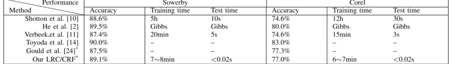
Table VI shows a comparison of results on Sowerby and Corel datasets. For Corel datasets, we do not use the pre-processing as described in [10], [24]. The accuracies within the ten randomly partition tests on Sowerby datasets are from 86.8% to 91.2%, and from 71.5% to 81.3% for Corel datasets, respectively. Fig.5 shows examples of the labeling results which obtained by the first stage LRC, the LRC/LRC and the LRC/CRF. The first stage LRC causes many isolated labels since it predicts the label of each patch independently. We can still find that the max-margin based CRF gives more “reasonable” results in most cases.
D. Discussion
This section analyzes and discusses some details of our segmentation method.
1) Classification based on concatenated bag of features and concatenated PLSA outputs: As described before, the dimension of features is significantly reduced by our topic probabilities based feature representation comparing with con-catenated words representation in [11], but how about the classification performance of these two representations for our semantic segmentation. We evaluate the performance of
(a) Image (b) LRC-I (c) LRC-II (d) LRC-II (e) CRF-II (f) CRF-II (g) GT
Fig. 3: Labeling samples for the MSRC-21 class datasets, below is the color-coding legend for the 21 object classes.Column (a) shows the original images to be labeled. Columns (b) shows the predictions of the first stage using LRC with the nearest interpolation mapping to pixels. Columns (c) and (d) show the predictions of the second stage using LRC with the nearest interpolation mapping and MRF smoothing mapping. Columns (e) and (f) show the predictions of the second stage using CRF with the nearest mapping and oversegmentation mapping. Columns (g) shows the hand labeling ground truth.
these two representations using the MSRC-9 dataset. Firstly, we use sift, color(hue descriptor) and gabor descriptor, and quantize them to 1000, 100 and 400 words, respectively. Each patch is then represented by the concatenated words (CW) or concatenated class probabilities (CP) predicted by PLSA classifier. Finally, we apply the logistic regression classifier to give the classification results. Table VII illustrates the dimensions of features, the classification accuracies and the computation cost. It shows the computation cost of CP is much lower than the CW. Another interesting point is that we
do not observe a drop in classification performance which is often experienced as a result of dimensionality reduction [38]. On the contrary, we get a slight lift in classification accuracy. This might be achieved by making better use of the available labeling information. Moreover, a lower dimensional feature representation speeds up computation, as seen in TableVII.
We also compare the performance of logistic regression classifier with multi-modal PLSA used in [16]. Table VIII gives the details. We find that the performance of multi-modal PLSA classifier is lower than the logistic regression classifier
(a) Image (b) LRC-I (c) LRC-II (d) LRC-II (e) CRF-II (f) CRF-II (g) GT
Fig. 4: Some difficult examples where labeling works less well, with corresponding color-coded output object-class maps.Column (a) shows the original images to be labeled. Columns (b) shows the predictions of the first stage using LRC with the nearest interpolation mapping to pixels. Columns (c) and (d) show the predictions of the second stage using LRC with the nearest interpolation mapping and MRF smoothing mapping. Columns (e) and (f) show the predictions of the second stage using CRF with the nearest mapping and oversegmentation mapping. Columns (g) shows the hand labeling ground truth.
when combining the two or three different descriptor, though they also assume that the different modalities are modeled as being independent given the patch label. We observe that LRC classifier with concatenating all the three feature channels gives the highest performance 77.1% in this comparison, while using multi-modal PLSA (mPLSA) with all the three channels leads to a slightly decrease (1.9%) in performance compared with combining only sift and color descriptor.
2) Comparison of Max-Likelihood and Max-Margin learn-ing: We use the stochastic gradient descent (SGD) method to
train the CRF model under the maximum likelihood learning framework, and select a suitable parameter 𝜂0 (gradient gain step) is the key to the computational speed and performance (to be set as high as possible while maintaining stability [42]). In our experiments, we use sum-product loopy belief propagation (SP LBP) to approximate the partition function and infer the labels. We set the gradient gain step 𝜂0 as 0.0001, and the maximum number of iterations for SGD is 40. The best result appears at the 35th iteration in this experiment.
As for the Max-margin learning method, we investigate several different energy optimization methods [52] (to infer the labels in step 1 of TableI), such as graph cuts (alpha-expansion for the non submodular case), FastPD, max-product LBP(MP LBP), and tree-reweighted message passing) as well
as the well-known older Iterated Conditional Modes (ICM) algorithm.
In this experiment, we explore two formulations of the energy function as follows,
Energy Formulation 1(EF-I):
𝐸(𝑥, 𝑦; w) = 𝑤1 ∑ 𝑖∈𝒱 − log 𝑃𝑠𝑖𝑓𝑡(𝑦𝑖∣𝑥𝑖)+ 𝑤2 ∑ 𝑖∈𝒱 − log 𝑃𝑐𝑜𝑙𝑜𝑟(𝑦𝑖∣𝑥𝑖) + 𝑤3 ∑ (𝑖,𝑗)∈ℰ 𝜓𝑖𝑗(𝑥𝑖, 𝑥𝑗) (11)
In this case,𝑤1,𝑤2 and𝑤3 are the coefficients that mod-ulate the effects of different potentials (two unary potentials (sift, color) and one pairwise potential),the energy in unary term is the negative log likelihood of sift or color descriptor given the label (i.e.,− log 𝑃 (𝑌 ∣𝑋). 𝑃 (𝑦𝑖∣𝑥𝑖) is the likelihood probability computed from the PLSA classifier. We just need to learn the coefficients𝑤1,𝑤2 and𝑤3, which modulate the effects of the different potentials.
TABLE II: Pixel level accuracy of segmentation for the MSRC-21 class dataset. The overall pixel-wise accuracy is 76.93% Inferr ed class True class b
uilding grass tree cow sheep sky aeroplane water face car bike flower sign bird book chair road cat dog body boat
building 62.8 1.7 10.5 0.1 0 3.2 0.2 2.1 2.6 0.4 3.5 0 0 0.1 2.3 1.4 7.6 0 0 1.2 0.3 grass 0.9 94.5 1.4 0.1 0.3 0.1 0.1 0.6 0 0 0 0.3 0 0 0 0 1.6 0 0 0.2 0 tree 2.2 6.7 82.1 0 0 2.6 0.2 0 0 0 0 4.2 0 0 0 0 0.6 0 0 1.3 0.1 cow 0 21.4 0.3 70.1 4.0 0 0 0.8 0 0 0 0.1 0 0 0 0 0.5 0.4 0.1 2.2 0 sheep 0 19.8 0 0.1 79.7 0 0 0 0 0 0.2 0 0 0 0 0 0.2 0 0 0 0 sky 1.7 0.1 0.5 0 0 92.2 0.1 0 0 0 0 0 0 5.1 0 0 0.3 0 0 0 0 aeroplane 23.6 10.4 0.8 0.8 0 5.0 56.4 0 0 0 0 0 0 0 0 0 3.0 0 0 0 0 water 3.3 3.4 6.3 0 0 2.8 0.2 66.5 0 0 0 0 0 2.8 0.9 0 13.4 0 0 0.4 0.1 face 4.2 0.4 4.0 0 0 1.1 0 0.3 72.4 0 0 0.3 0 0 3.9 0.1 0.1 0 6.9 6.2 0 car 12.1 0 2.0 0 0 0.1 0 0.0 0 62.6 0 0 0 0.6 0 0.2 15.0 5.8 0 0 1.6 bike 5.7 0.3 0.8 0 0 0 0 0 0 0.4 70.1 0 0 0 0 9.0 13.6 0 0 0 0 flower 0 0.4 1.9 0 0 0 0 0 0 0 0 97.6 0 0 0 0 0 0 0 0.1 0 sign 40.4 0.1 1.4 0 0 1.6 0 0 0 0 0 4.2 42.7 0 9.0 0 0.3 0.1 0 0.3 0 bird 4.6 11.5 3.5 0.9 0.8 3.2 3.0 5.9 0 3.5 0 6.5 0 43.5 0 7.8 4.3 0 0 0 1.0 book 3.1 0.1 0 0 0 0.2 0 0 0.2 0 0 0 0 0 96.1 0 0.1 0 0 0.2 0 chair 0.4 19.3 7.3 4.4 0 0 0 3.6 0 0 2.1 0 0.9 1.2 2.4 53.5 4.8 0 0 0 0 road 4.0 2.0 1.1 0 0 1.7 0.0 8.6 0.1 0.7 1.0 0 0 0 0 0.1 80.2 0 0 0.4 0 cat 3.0 0.1 0.3 0 0 0.6 0 5.4 0 0 0.4 0 0 4.0 0 0 12.1 74.1 0 0 0 dog 2.4 5.1 3.0 7.4 0 0.5 0 16.1 7.2 0 4.0 0 0 1.7 0.4 0 10.7 3.8 35.1 2.7 0 body 7.1 6.5 10.7 0.7 0 0.4 0 6.3 4.1 0 0 1.0 0 0.4 5.7 1.9 3.8 0 4 45.8 1.4 boat 29.8 0.1 0 0 0 2.2 0.5 28.8 0 1.5 5.7 0 0 1.8 0 0 9.6 0 0 2.2 17.9
TABLE III: Comparison of pixel-level accuracy to other algorithms on the MSRC-21 class dataset
Algorithm TextonBoost [10] PLSA-MRF [16] Meanshift [12] STF-ILP [22] AC(ACP) [21] RLP-CRF [24]* Our LRC/CRF*
Accuracy 72.2% 73.5% 75.1% 72% 74.5%(77.7%) 76.5% 76.8%
*For these two works, results are reported over five separate random partitions, other works are only reported on a single fold.
𝐸(𝑥, 𝑦; 𝛼, 𝑤𝑝) = ∑ 𝑖∈𝒱 𝑁 ∑ 𝑛=1 (𝛼𝑛𝑙𝑦𝑖𝑛) + 𝑤𝑝 ∑ (𝑖,𝑗)∈ℰ 𝜓𝑖𝑗(𝑥𝑖, 𝑥𝑗) (12) where𝑦𝑖 denotes a𝑁-dimensional concatenated probability vector of PLSA output using sift and color descriptor, 𝑥𝑖 ∈
{1, ⋅ ⋅ ⋅ , 𝑙, ⋅ ⋅ ⋅ , 𝐿} denote the label of node 𝑖, and 𝛼𝑛𝑙is𝑁 ×𝐿
matrix of coefficients to be learned. Here,𝐿 = 9(for MSRC-9 class data, the number of object classes we consider is MSRC-9),
𝑁 = 18, thus in this case, we need to learn 162 parameters
for the unary term and𝑤𝑝 for the pairwise term.
The pairwise terms are both the simple Potts model, and for simplicity, we just take the sift (1000 words) and color descriptor (100 words) as features in this experiment, the patch-level labeling accuracy and running time are shown in Table IX. Experimental results show that margin-maximization approaches can be more accurate than likelihood-maximization approaches for training discriminative classifiers, and perfor-mance of the second energy formulation outperforms the first one by 2-3%. Among the several energy optimization methods [52], the FastPD algorithm gives the competitive performance and the lowest computation cost.
3) Benefits of the position information and context informa-tion: Fig.6 shows the effects of using different neighborhood systems in MSRC-9 and MSRC-21 class datasets. Here we first explain the meaning of each label in x-axis of Fig.6,
∙ N0-I: LRC with concatenated output of the three in-dependent PLSA classifier on the sift, color and gabor descriptor;
∙ N0-II: N0-I + the spatial layout labels information;
∙ N0: N0-II + the image-level global aggregate information;
∙ N1-N5: N0 + regional information with 1-5 order neigh-borhood system. N0−I N0−II N0 N1 N2 N3 N4 N5 0.6 0.625 0.65 0.675 0.7 0.725 0.75 0.775 0.8 0.825 0.85 0.875 0.9 0.925 0.95 MSRC datasets
N−order neighbor system
Mean average precision
Stage2−LRC(MSRC−9) Stage2−CRF(MSRC−9) Stage2−LRC(MSRC−21) Stage2−CRF(MSRC−21)
TABLE V: Comparison of pixel-level labeling accuracy to other algorithms on MSRC-9 class dataset(%)
Object
class
Method
b
uilding grass tree cow sky aeroplane face car bicycle per
pixel Schroff et al. [50] 56.7 84.8 76.4 83.8 81.1 53.8 68.5 71.4 72.0 75.2 PLSA-MRF [16]a 74.0 88.7 64.4 77.4 95.7 92.2 88.8 81.1 78.7 82.3 CRF [11]a 73.6 91.1 82.1 73.6 95.7 78.3 89.5 84.5 81.4 84.9 LTRF [19] 78.1 92.5 85.4 86.7 94.6 77.9 83.5 74.7 88.3 86.7 RF-CRF [13] – – – – – – – – – 87.2 RLP-CRF [24]b – – – – – – – – – 88.5 Our LRC/CRF-avea 82.4 93.9 85.2 81.8 93.8 76.0 92.6 90.2 88.5 88.6 Our LRC/CRF-min 79.5 90.8 87.9 77.7 90.7 72.6 91.2 82.6 95.2 86.6 Our LRC/CRF-max 86.6 94.7 87.7 87.7 91.8 83.5 98.8 92.4 86.3 90.7
aFor these three works, results are reported over 20 random train-test partitions bFor this work, result is reported over 5 random train-test partitions
Fig. 5: Labeling results for the Sowerby and Corel data sets with the legends. Column (a) shows the original images to be labeled. Columns (b) shows the predictions of the first stage using LRC with the nearest interpolation mapping to pixels. Columns (c) show the predictions of the second stage using LRC with the MRF smoothing mapping. Columns (d) shows the predictions of the second stage using CRF with the oversegmentation mapping. Columns (e) shows the hand labeling ground truth.
With the introduction of spatial layout labels information, the performances are significantly improved on both datasets. With the LRC, it achieves 4.4% and 8.65% performance gain for MSRC-9 and MSRC-21 datasets, respectively. Using CRF also gives 3.44% and 6.46% improvement in these two datasets.
The performance increment from the image-level global aggregate information by CRF is lower than LRC. With LRC, it respectively increases the accuracy by 0.93% and 2.1% for MSRC-9 and MSRC-21 datasets. Using the CRF, the improvements of accuracy are 0.58% and 0.74% , respectively.
TABLE VI: Comparison of pixel level labeling accuracy to other algorithms on the Sowerby and Corel datasets
``````Method Performance``` Sowerby Corel
Accuracy Training time Test time Accuracy Training time Test time Shotton et al. [10] 88.6% 5h 10s 74.6% 12h 30s
He et al. [2] 89.5% Gibbs Gibbs 80.0% Gibbs Gibbs Verbeek,et al. [11] 87.4% 20min 5s 74.6% 15min 3s
Toyoda et al. [14] 90.0% – – 83.0% – – Gould et al. [24]* 87.5% – – 77.3% – –
Our LRC/CRF* 89.1% 7∼8min <0.02s 77.0% 6∼7min <0.02s *For these two works, results are reported over 10 random train-test partitions, other works are only reported on a single fold.
TABLE VII: Patch-level performances under concatenated words and concatenated predicted class probabilities, with sift, color and gabor descriptor.
Performance CW-SC CW-SCG CP-SC CP-SCG local local+global local local+global local local+global local local+global Dimensions 1100 2200 1500 3000 18 36 27 54 Accuracy(%) 62.2 75.1 63.2 77.5 74.7 76.8 77.1 79.6
Cpu time(s) 7.67 197.06 14.05 1696.34 4.80 6.46 5.77 8.42
TABLE VIII: Patch-level accuracies under PLSA, mPLSA and LRC on topic vectors learned from labeled patches, with various combinations of the three modalities SIFT, Color and Gabor
Descriptor SIFT Color Gabor SC SG CG SCG Classifier PLSA PLSA PLSA LRC mPLSA LRC mPLSA LRC mPLSA LRC mPLSA Accuracy(%) 60.1 59.1 52.8 74.7 73.8 65.5 56.4 73.6 70.3 77.1 71.9
Cpu time(s) 0.79 0.27 0.53 4.80 41.87 4.97 51.43 4.92 22.59 5.77 59.46
TABLE IX: Patch-level performances of CRF learning by likelihood maximization (ML) method and margin-maximization (MM) method, with sift and color descriptors on MSRC-9 class data.
Method ML-SP LBP MM-ICM MM-MP LBP MM-TRWS MM-GC MM-FastPD EF-I EF-II EF-I EF-II EF-I EF-II EF-I EF-II EF-I EF-II* EF-I EF-II
Accuracy(%) 76.3 78.9 75.4 77.9 76.8 79.3 77.0 79.5 76.9 – 76.9 79.6 Cpu time(s) 6954.52 7288.38 307.38 205.35 5041.94 3290.16 2471.39 2122.88 140.81 – 100.24 150.88
*alpha-expansion got a situation in this case because of the computed energy breaks through the third constraint on the smoothing term [47], i.e.the
triangle rule:𝑉 (𝛼, 𝛽) ≤ 𝑉 (𝛼, 𝛾) + 𝑉 (𝛾 + 𝛽).It is mostly due to the updating of weights using Max-margin learning with SVM struct is arbitrary. In addition, the constraints on the pairwise term added by SVM struct are SOFT constraints (i.e. they have a slack variable). So, they can be violated. i.e. even if given the positive constraints on the pairwise term weights, it can still get negative weights in some case.
Let us now focus on the effect of different neighborhood systems, we can observe that using more than 2-order neighbor system, the performance is near saturation for MSRC-9 class dataset. For the MSRC-21 class dataset, the performance lifts off on the 4-order system. The 1-order neighborhood information gives the maximum gain in both datasets, 2.2% for MSRC-9 and 0.6% for MSRC-21.
It is also interesting to note that after adding the spatial layout labels information and image-level global aggregate information, the performances obtained by LRC and CRF in the second stage are very close.
Note that in the case of N0-I, the performance for MSRC-9 has reached 82.1%, which is 5% outperform the 77.1% in TableVIII although they use the similar three descriptors, because here we use a combination of hue descriptor and opponent angle as the color descriptor, and we also test with a larger codebook size (1000).
VI. CONCLUSION
Segmentation of images into disjoint regions and interpreta-tion of the regions for semantic meanings are two central tasks
in an image analysis system. We have presented a fast high per-formance approach to semantic image labeling that incorporate the local, regional and global features. Our model encodes regional and global information as local features enabling us to use much simpler probabilistic models, such as logistic regression, while still achieving state-of-the-art performance. The results show to significantly improve the results by patch-based classification algorithms and demonstrate comparable performance to state of the art [21] [24]. We also show that existing software that is high in quality and easy to use, specifically the well known “LIBLINEAR” package [49] and “SVMStruct” package [6], can be used together to achieve high performance and high speed on semantic segmentation task that so far has been addressed only using complex custom methods that are effectively out of reach for practitioners. From this situation, we feel that many useful optimization techniques have not been fully exploited for computer vision applications.
One limit of our method is that the dimensionality of patch representation will increase linearly with the number of object classes in the dataset. It might seem that this low
dimensional semantic representation will be also ineffective to very large scale problems with thousands of object classes. Another limitation of our approach is that the images are represented as rectangular patches at a single scale which could not capture many classes whose appearance and co-occurrence varies significantly with scale. One way to capture this would be to learn separate topic models for the patch appearances or label mixtures at each scale, and use these as features. We intend to explore this in future work.
ACKNOWLEDGMENT
The authors would like to thank Prof. Joachims of Cornell University for his helpful discussions on using SVM struct. This research were supported in part by CLASS (IST project 027978, funded by the European Union Information Society Technologies unit E5 C Cognition) and the National Natural Science Foundation of China (No.40801183,60890074).
REFERENCES
[1] A. Criminisi, Microsoft research Cambridge object recognition image database (version 1.0 and 2.0), 2004. http://research.microsoft.com/vision/cambridge/recognition.
[2] X. He, R.S. Zemel, and M. ´A.Carreira-Perpinan, “ Multiscale Conditional Random Fields for Image Labeling,” in Proc. IEEE CS Conf. Computer
Vision and Pattern Recognition, vol. 2, pp. 695-702, 2004.
[3] N. Komodakis and G. Tziritas, “ Approximate Labeling via Graph-Cuts Based on Linear Programming,” IEEE Trans. Pattern Anal. Mach. Intell., vol.29, no. 8, pp. 1436-1453, Aug.2007.
[4] M. Szummer, P. Kohli, and D. Hoiem, “ Learning CRF using Graph Cuts,” in Proc. Tenth European Conf. Computer Vision, 2008. [5] T. Finley and T. Joachims, “ Training Structural SVMs when Exact
Inference is Intractable,” in Proc.25th Int’l Conf. Machine Learning, pp. 304-311, 2008.
[6] T. Joachims, T. Finley and C.N. Yu, “ Cutting-Plane Training of Structural SVMs,” Machine Learning, vol.76,no.1,2009.
[7] X. He, R.S. Zemel, and D. Ray, “ Learning and Incorporating Top-Down Cues in Image Segmentation,” in Proc. Ninth European Conf. Computer
Vision, vol. 1, pp. 338-351, 2006.
[8] S. Kumar and M. Hebert, “ A Hierarchical Field Framework for Unified Context-Based Classification,” in Proc. 10th Int’l Conf. Computer Vision, vol. 2, pp. 1284-1291, 2005.
[9] A. Torralba, K.P. Murphy, and W.T. Freeman, “ Contextual Models for Object Detection Using Boosted Random Fields,” in Advances in Neural
Information Processing Systems, vol. 17, pp. 1401-1408, 2005.
[10] J. Shotton, J. Winnand, C. Rother, and A. Criminisi, “ Textonboost: Joint Appearance, Shape and Context Modeling for Multi-Class Object Recognition and Segmentation,” in Proc. Ninth European Conf.
Com-puter Vision, vol. 1, pp. 1-15, 2006.
[11] J.Verbeek, B. Triggs, “ Scene Segmentation with CRF Learned from Par-tially Labeled Images,” in Advances in Neural Information Processing
Systems, pp.1553-1560, MIT Press, 2008.
[12] L.Yang, P.Meer, and D.J.Foran. “ Multiple class segmentation using a unified framework over mean-shift patches,” in Proc. IEEE CS Conf.
Computer Vision and Pattern Recognition. pp.1-8, 2007.
[13] F.Schroff, A. Criminisi, and A. Zisserman, “ Object Class Segmentation using Random Forests,” in Proc. British Machine Vision Conf. 2008 [14] T.Toyoda, O.Hasegawa “ Random Field Model for Integration of Local
Information and Global Information,” IEEE Trans. Pattern Anal. Mach.
Intell., vol. 30, no. 8, pp. 1483-1480, Aug. 2008
[15] A. Rabinovich, A. Vedaldi, C. Galleguillos, E. Wiewiora and S. Be-longie. “ Objects in Context,” in Proc. 11th Int’l Conf. Computer Vision, 2007
[16] J. Verbeek, B. Triggs, “ Region Classification with Markov Field Aspect Models,” in Proc. IEEE CS Conf. Computer Vision and Pattern
Recognition. 2007.
[17] L. Cao and L. Fei-Fei, “ Spatially Coherent Latent Topic Model for Concurrent Segmentation and Classification of Objects and Scenes,” in
Proc. 11th Int’l Conf. Computer Vision, 2007.
[18] X. He, R.S. Zemel, “ Latent Topic Random Fields: Learning using a taxonomy of labels,” in Proc. IEEE CS Conf. Computer Vision and
Pattern Recognition, 2008
[19] X. He, R.S. Zemel, “ Learning Hybrid Models for Image Annotation with Partially Labeled Data,” in Advances in Neural Information
Pro-cessing Systems, 2008
[20] G. Csurka and F. Perronnin, “ A Simple High Performance Approach to Semantic Segmentation,” in Proc. British Machine Vision Conf. 2008. [21] Z.W. Tu, “ Auto-context and Its application to High-level Vision Tasks,”
in Proc. IEEE CS Conf. Computer Vision and Pattern Recognition, 2008 [22] J. Shotton, M. Johnson, R. Cipolla. “ Semantic Texton Forests for Image Categorization and Segmentation,” in Proc. IEEE CS Conf. Computer
Vision and Pattern Recognition, 2008
[23] C.Galleguillos, A.Rabinovich, S.Belongie, “ Object Categorization using Co-Occurrence, Location and Appearance,” in Proc. IEEE CS Conf.
Computer Vision and Pattern Recognition, 2008.
[24] S. Gould, J. Rodgers, D. Cohen, G. Elidan, D. Koller, “ Multi-Class Segmentation with Relative Location Prior,” Int’l J. Computer Vision, vol. 80, no.3, pp. 300-316, 2008
[25] D. Lowe, “ Distinctive image features from scale-invariant keypoints,”
Int’l J. Computer Vision, vol. 60, no. 2, pp. 91-110, 2004
[26] V. Kyrki, J. K. K¨am¨ar¨ainen, H. K¨alvi¨ainen, “ Simple Gabor Feature Space for Invariant Object Recognition,” Pattern Recognit. Lett., vol. 25, no.3, pp. 311-318, 2004.
[27] J. van de Weijer, C. Schmid, “ Coloring Local Feature Extraction,” in
Proc. Ninth European Conf. Computer Vision, vol.2, pp.334-348, 2006.
[28] T. Hofmann. “ Unsupervised learning by probabilistic latent semantic analysis,” Machine Learning, vol.42, no.1-2, pp.177-196, 2001. [29] D. Blei, A. Ng, and M. Jordan. “ Latent Dirichlet allocation,” J.Machine
Learning Research, no.3, pp.993-1022, 2003.
[30] P. Quelhas, F. Monay, J.-M. Odobez, D. Gatica-Perez, T. Tuytelaars, and L. Van Gool. “ Modeling scenes with local descriptors and latent aspects,” in Proc. 10th Int’l Conf. Computer Vision, vol.1,pp.883-890, 2005.
[31] A. Bosch, A. Zisserman, and X. Munoz. “ Scene classification via plsa,” in Proc. Ninth European Conf. Computer Vision, pp.517-530, 2006. [32] F.-F. Li and P. Perona. “ A bayesian hierarchical model for learning
natural scene categories,” in Proc. IEEE CS Conf. Computer Vision and
Pattern Recognition, pp.524-531, 2005.
[33] N.Rasiwasia, N.Vasconcelos, “ Scene classification with low-dimensional semantic spaces and weak supervision,” in Proc. IEEE CS
Conf. Computer Vision and Pattern Recognition, 2008.
[34] E. Xing, R. Yan, and A. Hauptmann, “ Mining associated text and images with dual-wing harmoniums,” in Proc. of the 21th Annual Conf. on
Uncertainty in Artificial Intelligence. AUAI press, 2005.
[35] W. Li , A. McCallum, “ Pachinko allocation: DAG-structured mixture models of topic correlations,” in Proc.23th Int’l Conf. Machine Learning, pp.577-584, 2006.
[36] S. Lazebnik and M. Raginsky, “ An Empirical Bayes Approach to Contextual Region Classification,” in Proc. IEEE CS Conf. Computer
Vision and Pattern Recognition, to appear 2009
[37] K. Grauman and T. Darrell. “ The Pyramid Match Kernel: Discriminative Classification with Sets of Image Features,” in Proc. 10th Int’l Conf.
Computer Vision, pp. 1458-1465, 2005.
[38] S. Lazebnik, C. Schmid, and J. Ponce. “ Beyond bags of features: Spatial pyramid matching for recognizing natural scene categories,” in Proc.
IEEE CS Conf. Computer Vision and Pattern Recognition, vol. 2, pp.
2169-2178, 2006.
[39] S.Z. Li,Markov Random Field Modeling In Image Analysis, the 2nd edition,Springer-Verlag Press,2001.
[40] C.-J. Lin, R. C. Weng, and S. S. Keerthi. “ Trust region Newton method for large-scale logistic regression,” J. Machine Learning Research, no.9,pp. 627-650,2008.
[41] J. Lafferty, A. McCallum, and F. Pereira. “ Conditional random fields: probabilistic models for segmenting and labeling sequence data,” in
Proc.18th Int’l Conf. Machine Learning, pp. 282-289, 2001.
[42] S.Vishwanathan, N. Schraudolph, M. Schmidt, K. Murphy, “ Accelerated Training of Conditional Random Fields with Stochastic Meta-Descent,” in Proc.23th Int’l Conf. Machine Learning, pp. 969-976, 2006. [43] B.Taskar, S. Lacoste-Julien, M. I. Jordan,“ Structured Prediction, Dual
Extragradient and Bregman Projections,” J. Machine Learning Research, no.7, pp.1627-1653, 2006.
[44] I.sochantaridis, T.Joachims, T.Hofmann, Y.Altun, “ Large margin meth-ods for structured and interdependent output variables,” J.Machine
[45] D.Anguelov, B.Taskar, V.Chatalbashev, D.Koller, D.Gupta, G.Heitz, A.Y. Ng, “ Discriminative learning of Markov random fields for segmentation of 3D scan data,” in Proc. IEEE CS Conf. Computer Vision and Pattern
Recognition, pp.169-176,2005
[46] B.Taskar, V.Chatalbashev, D.Koller, C.Guestrin, “ Learning structured prediction models: a large margin approach,” in Proc.22th Int’l Conf.
Machine Learning, pp.896-903,2005.
[47] Y.Boykov, O.Veksler, R. Zabih, “ Fast approximate energy minimization via graph cuts,” IEEE Trans. Pattern Anal. Mach. Intell., vol. 23, no. 11, pp. 1222-1239, Nov. 2001.
[48] N. Komodakis, G. Tziritas and N. Paragios, “ Performance vs Compu-tational Efficiency for Optimizing Single and Dynamic MRFs: Setting the State of the Art with Primal Dual Strategies,” Computer Vision and
Image Understanding, vol.112, no.1, pp.14-29, Oct. 2008.
[49] R.E. Fan, K.W. Chang, C.J. Hsieh, X.R. Wang, and C.J. Lin. “ LIB-LINEAR: A library for large linear classification,” J. Machine Learning
Research, no.9, pp.1871-1874, 2008.
[50] F. Schroff, A. Criminisi, and A. Zisserman. “ Single-histogram class models for image segmentation,” in Proc.Indian Conf. Computer Vision,
Graphics and Image Processing, 2006.
[51] D.Comaniciu and P.Meer, “ Mean Shift: A Robust Approach toward Feature Space Analysis,” IEEE Trans. Pattern Anal. Mach. Intell., vol. 24, no. 5, pp. 603-619, May 2002.
[52] R. Szeliski, R. Zabih, D. Scharstein, O. Veksler, V. Kolmogorov, A. Agarwala. “ A comparative study of energy minimization methods for Markov random fields,” IEEE Trans. Pattern Anal. Mach. Intell., vol.30, no.6, pp.1068-1080, 2008.
Wen YANGreceived his Ph.D degree from Wuhan University, China, in 2004. He is currently an as-sociate professor at the School of Electronic In-formation, Wuhan University. His research interests include image segmentation and classification, target detection and recognition, machine learning and data mining with applications to remote sensing.
Bill Triggs originally trained as a mathematical physicist at Auckland, Australian National, and Ox-ford Universities. He has worked extensively on vision geometry (matching constraints, scene re-construction, autocalibration) and robotics, but his current research focuses on computer vision, pattern recognition, and machine learning for visual object recognition and human motion understanding. Now he works in (and is deputy director of) the Labora-toire Jean Kuntzmann (LJK) in Grenoble in the heart of the French Alps.
Dengxin Dai received B.S. degree in optical in-formation science and technology in 2008, from Wuhan University, Wuhan, Hubei, China, where he is currently working toward the Ph.D degree at the signal processing laboratory, school of electronic information. His research interests include image processing, computer vision, and machine learning.
Gui-Song Xia received the B.S and M.S. degree in Electronic Engineering from Wuhan University, Wuhan, China, in 2005 and 2007, respectively. He is currently pursuing his Ph.D degree at French National Center for Scientific Research (CNRS) -Information Processing and Communication Labora-tory (LTCI), Institute Telecom, Telecom ParisTech, Paris, France. His research interests include image analysis, computer vision, learning in vision, image processing and remote sensing.