HAL Id: hal-01055789
https://hal.inria.fr/hal-01055789
Submitted on 13 Aug 2014HAL is a multi-disciplinary open access archive for the deposit and dissemination of sci-entific research documents, whether they are pub-lished or not. The documents may come from teaching and research institutions in France or abroad, or from public or private research centers.
L’archive ouverte pluridisciplinaire HAL, est destinée au dépôt et à la diffusion de documents scientifiques de niveau recherche, publiés ou non, émanant des établissements d’enseignement et de recherche français ou étrangers, des laboratoires publics ou privés.
Conciliation d’a prioris sans préjugé
Rémi Gribonval, Pierre Machart
To cite this version:
Rémi Gribonval, Pierre Machart. Conciliation d’a prioris sans préjugé. 46è Journées de Statistique, Jun 2014, Rennes, France. �hal-01055789�
Conciliation d’
a prioris sans pr´ejug´e
R´emi Gribonval∗
& Pierre Machart∗
∗
INRIA, Centre de Rennes - Bretagne Atlantique, prenom.nom@inria.fr
R´esum´e. Il existe deux grandes familles de m´ethodes pour r´esoudre les probl`emes
lin´eaires inverses. Tandis que les approches faisant appel `a la r´egularisation construisent des estimateurs comme solutions de probl`emes de r´egularisation p´enalis´ee, les estimateurs Bay´esiens reposent sur une distribution post´erieure de l’inconnue, ´etant donn´ee une famille suppos´ee d’a priori. Bien que ces approchent puissent paraˆıtre radicalement diff´erentes, des r´esultats r´ecents ont montr´e, dans un contexte de d´ebruitage additif Gaussien, que l’estimateur Bay´esien d’esp´erance conditionnelle est toujours la solution d’un probl`eme de r´egression p´enalis´ee. Nous prsentons deux contributions. D’une part, nous ´etendons le r´esultat valable pour le bruit additif gaussien aux probl`emes lin´eaires inverses, plus g´en´eralement, avec un bruit Gaussien color´e. D’autre part, nous caract´erisons les con-ditions sous lesquelles le terme de p´enalit´e associ´e `a l’estimateur d’esp´erance condition-nelle satisfait certaines propri´et´es d´esirables comme la convexit´e, la s´eparabilit´e ou la diff´erentiabilit´e. Cela permet un ´eclairage nouveau sur certains compromis existant en-tre efficacit´e computationnelle et pr´ecision de l’estimation pour la r´egularisation parci-monieuse, et met `a jour certaines connexions entre estimation Bay´esienne et optimisation proximale.
Mots-cl´es. probl`emes lin´eaires inverses, estimation Bay´esienne, maximum a
posteri-ori, estimateur d’esp´erance conditionnelle, moindres carr´es p´enalis´es
Abstract. There are two major routes to address linear inverse problems. Whereas
regularization-based approaches build estimators as solutions of penalized regression op-timization problems, Bayesian estimators rely on the posterior distribution of the un-known, given some assumed family of priors. While these may seem radically different approaches, recent results have shown that, in the context of additive white Gaussian denoising, the Bayesian conditional mean estimator is always the solution of a penal-ized regression problem. We present two contributions. First, we extend the additive white Gaussian denoising results to general linear inverse problems with colored Gaussian noise. Second, we characterize conditions under which the penalty function associated to the conditional mean estimator can satisfy certain popular properties such as convexity, separability, and smoothness. This sheds light on some tradeoff between computational efficiency and estimation accuracy in sparse regularization, and draws some connections between Bayesian estimation and proximal optimization.
Keywords. linear inverse problems, Bayesian estimation, maximum a posteriori,
This long abstract aims at introducing partially published results. For the sake of conci-sion, no element proof will be provided here. However, extensive proofs for the mentionned results can be found in our NIPS paper [1] and research report [2].
1
Introduction
Let us consider a fairly general linear inverse problem, where one wants to estimate a
parameter vector z ∈ RD
, from a noisy observation y ∈ Rn
, such that y = Az + b,
where A ∈ Rn×D is sometimes referred to as the observation or design matrix, and
b∈ Rn represents an additive noise.When n < D, it turns out to be an ill-posed problem.
However, leveraging some prior knowledge or information, a profusion of schemes have been developed in order to provide an appropriate estimation of z. In this abundance, we will focus on two seemingly very different approaches.
Two families of approaches for linear inverse problems On the one hand, Bayesian
approaches are based on the assumption that z and b are drawn from probability
distri-butions PZ and PB respectively. From that point, a straightforward way to estimate z
is to build, for instance, the Minimum Mean Squared Error (MMSE) estimator, some-times referred to as Bayesian Least Squares, conditional expectation or conditional mean estimator, and defined as:
ψMMSE(y) := E(Z|Y = y). (1)
This estimator has the nice property of being optimal (in a least squares sense) but suffers from its explicit reliance on the prior distribution, which is usually unknown. Moreover, its computation involves an integral computation that generally cannot be done explicitly. On the other hand, regularization-based approaches have been at the centre of a tremendous amount of work from a wide community of researchers in machine learning, signal processing, and more generally in applied mathematics. These approaches focus on building estimators (also called decoders) with no explicit reference to the prior distribu-tion. Instead, these estimators are built as some optimal trade-off between a data fidelity term and some term promoting some regularity on the solution. Among these, we will focus on a particularly widely studied family of estimators ψ that write in this form:
ψ(y) := argmin
z∈RD
1
2ky − Azk
2+ φ(z). (2)
For instance, the specific choice φ(z) = λkzk2
2 gives rise to a method often referred to as
the ridge regression [3] while φ(z) = λkzk1 gives rise to the famous Lasso [4].
Do they really provide different estimators? Regularization and Bayesian
underpinned by distinct ways of defining signal models or “priors”. The “regularization prior” is embodied by the penalty function φ(z) which promotes certain solutions, carving an implicit signal model. In the Bayesian framework, the “Bayesian prior” is embodied
by where the mass of the signal distribution PZ lies.
The MAP quid pro quo A quid pro quo between these distinct notions of priors
has crystallized around the notion of maximum a posteriori (MAP) estimation, leading to a long lasting incomprehension between two worlds. In fact, a simple application of Bayes rule shows that under a Gaussian noise model b ∼ N (0, I) and Bayesian prior
PZ(z ∈ E) =
R
EpZ(z)dz, E ⊂ R
N
, MAP estimation1 yields the optimization problem (2)
with regularization prior φZ(z) := − log pZ(z). By a trivial identification, the
optimiza-tion problem (2) with regularizaoptimiza-tion prior φ(z) is now routinely called “MAP with prior
exp(−φ(z))”. With the ℓ1 penalty, it is often called “MAP with a Laplacian prior”. As
an unfortunate consequence of an erroneous “reverse reading” of this fact, this identifica-tion has given rise to the erroneous but common myth that the optimizaidentifica-tion approach is particularly well adapted when the unknown is distributed as exp(−φ(z)).
In fact, [5] warns us that the MAP estimate is only one of the plural possible Bayesian interpretations of (2), even though it certainly is the most straightforward one. Taking one step further to point out that erroneous conception, a deeper connection is dug, showing that in the more restricted context of (white) Gaussian denoising, for any prior, there exists a regularizer φ such that the MMSE estimator can be expressed as the solution of problem (2). This result essentially exhibits a regularization-oriented formulation for which two radically different interpretations can be made. It highlights the important following fact: the specific choice of a regularizer φ does not, alone, induce an implicit prior
on the supposed distribution of the unknown; besides a prior PZ, a Bayesian estimator
also involves the choice of a loss function. For certain regularizers φ, there can in fact
exist (at least two) different priors PZ for which the optimization problem (2) yields the
optimal Bayesian estimator, associated to (at least) two different losses (e.g.., the 0/1 loss for the MAP, and the quadratic loss for the MMSE).
2
Contributions
Main result A first major contribution of our recent paper [1] is to extend the result
of [5] to a more general linear inverse problem setting (i.e. y = Az + b). In a nutshell, it
states that for any prior PZ on z, the MMSE estimate with Gaussian noise PB = N (0, Σ)
is the solution of a regularization-formulated problem (though the converse is not true).
Theorem 1 (Main result). For any non-degenerate prior2 P
Z, any non-degenerate noise
covariance Σ and observation matrix A, we have: 1. ψMMSE is injective.
2. There exists a C∞
function φMMSE, such that for all vector y ∈ Rn, ψMMSE(y) is the unique
global minimum and stationary point of z 7→ 1
2ky − Azk
2
Σ+ φMMSE(z).
3. When A is invertible, φMMSE is uniquely defined, up to an additive constant.
For further details about the characterization of φMMSE(z), see [2]. It is worth noting
that its construction uses techniques going back to Stein’s unbiased risk estimator [6].
Connections between the MMSE and regularization-based estimators Some
simple observations of the main theorem can shed some light on connections between the MMSE and regularization-based estimators. For any prior, as long as A is invertible, there exists a corresponding regularizing term. It means that the set of MMSE estimators in linear inverse problems with Gaussian noise is a subset of the set of estimators that are produced by a regularization approach with a quadratic data-fitting term.
Second, since the corresponding penalty is necessarily smooth, it is in fact only a
strict subset of such regularization estimators. In other words, for some regularizers,
there cannot be any interpretation in terms of an MMSE estimator. For instance, as
pinpointed by [5], all the non-C∞
regularizers belong to that category. Among them,
all the sparsity-inducing regularizers (e.g. ℓ1 norm) fall into this scope. This means
that when solving a linear inverse problem (with an invertible A) under Gaussian noise, sparsity inducing penalties are necessarily suboptimal (in a mean squared error sense).
Relating desired computational properties to the evidence Let us now focus on
the MMSE estimators (which also can be written as regularization-based estimators). As reported in the introduction, one of the reasons explaining the success of optimization-based approaches is that one can have a better control on the computational efficiency of the algorithms via some appealing properties of the functional to minimize. An interesting question then is: can we relate these properties of the regularizer to the Bayesian priors, when interpreting the solution as an MMSE estimate?
For instance, when the regularizer is separable, one may easily rely on coordinate descent algorithms [7]. Even more evidently, when solving optimization problems, dealing with convex functions ensures that many algorithms will provably converge to the global minimizer [8]. As a consequence, it is interesting to characterize the set of priors for which the MMSE estimate can be expressed as a minimizer of a convex or separable function.
The following lemma precisely addresses these issues. For the sake of simplicity and readability, we focus on the specific case where A = I and Σ = I.
2We only need to assume that Z does not intrinsically live almost surely in a lower dimensional
hyper-plane. The results easily generalize to this degenerate situation by considering appropriate projections of y and z. Similar remarks are in order for the non-degeneracy assumptions on Σ and A.
Lemma 1 (Convexity and Separability). For any non-degenerate prior PZ, Theorem 1
in [2] says that ∀y ∈ Rn, ψ
I,I,PZ(y) is the unique global minimum and stationary point of
z 7→ 1
2ky − Izk2+ φI,I,PZ(z). Moreover, the following results hold:
1. φI,I,PZ is convex if and only if pY(y) := pB⋆ PZ(y) is log-concave,
2. φI,I,PZ is additively separable if and only if pY(y) is multiplicatively separable.
From this result, one may also draw an interesting negative result. If the distribution of the observation y is not log-concave, then, the MMSE estimate cannot be expressed as the solution of a convex regularization-oriented formulation. This means that, with a quadratic data-fitting term, a convex approach to signal estimation cannot be optimal (in a mean squared error sense). One may also note that the properties of the regularizer
explicitly rely on properties of the evidence pY rather than these of the prior PZ directly.
This is reminiscent of former interesting results in [9].
3
Worked example : the Bernoulli-Gaussian model
It is worth noting that the results of this section (and further details about them) can be found in our research report [2]. However, they are currently unpublished. The Bernoulli-Gaussian prior corresponds to the specific case of a 1-D mixture of a Dirac (with a weight
p) a Gaussian. This prior is often used as marginal distribution to model high-dimensional
sparse data, as the value z = 0 is drawn with a probability p > 0. Naturally, this prior is
not log-concave for any p > 0. However, due to its smoothing effect, the evidence pY can
still be log-concave as long as the noise level is high enough.
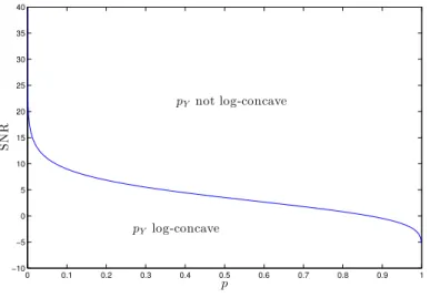
We obtain Figure 1 depicting the maximal signal-to-noise ratio (SNR) ensuring that
the evidence pY is log-concave, as a function of the sparsity level p. We notice that when
p→ 0 (i.e., the signal is not sparse), the maximal SNR goes to +∞. This means that for
any level of noise, the evidence (which becomes a simple Gaussian) becomes log-concave. On the other hand, when p → 1 (i.e. the signal is very sparse), the maximal SNR goes to −∞. Moreover, the curve is monotonically decreasing with p. In other words, the higher the sparsity level, the lower the SNR (hence the higher the noise level) needs to be to
ensure that the evidence pY is log-concave. Furthermore, one can note that even for a
relatively low level of sparsity, say 0.1, the evidence pY cannot be log-concave unless the
SNR is smaller than 9dB. As a consequence, when using penalized least-squares methods with a convex regularizing term, the resulting estimator cannot be optimal (in a mean squared error sense) unless the observations are very noisy, which basically means that the performances will be poor anyway.
0 0.1 0.2 0.3 0.4 0.5 0.6 0.7 0.8 0.9 1 −10 −5 0 5 10 15 20 25 30 35 40 p S N R pY not log-concave pYlog-concave
Figure 1: A plot of the maximal SNR so that pY is log-concave (hence φ is convex)
References
[1] R´emi Gribonval and Pierre Machart. Reconciling “priors” & “priors” without prejudice? In in Adv. Neural Information Processing Systems (NIPS), 2013.
[2] R´emi Gribonval and Pierre Machart. Reconciling “priors” & “priors” without prejudice? Technical report, INRIA Rennes - Bretagne Atlantique, 2013.
[3] Arthur E. Hoerl and Robert W. Kennard. Ridge regression: applications to nonorthogonal problems. Technometrics, 12(1):69–82, 1970.
[4] Robert Tibshirani. Regression shrinkage and selection via the lasso. Journal of the Royal Statistical Society, 58(1):267–288, 1996.
[5] R´emi Gribonval. Should penalized least squares regression be interpreted as maximum a posteriori estimation? IEEE Transactions on Signal Processing, 59(5):2405–2410, 2011. [6] Charles M. Stein. Estimation of the mean of a multivariate normal distribution. Annals of
Statistics, 9(6):1135–1151, 1981.
[7] Yurii Nesterov. Efficiency of coordinate descent methods on huge-scale optimization prob-lems. Core discussion papers, Center for Operations Research and Econometrics (CORE), Catholic University of Louvain, 2010.
[8] Stephen Boyd and Lieven Vandenberghe. Convex Optimization. Cambridge University Press, 2004.
[9] Martin Raphan and Eero P. Simoncelli. Learning to be bayesian without supervision. In in Adv. Neural Information Processing Systems (NIPS). MIT Press, 2007.