Analysis of Texture Evolution and Hardening Behavior during
Deep Drawing with an Improved Mixed Type FEM Element
Laurent Duchêne
ʆ, Pierre de Montleau*, Fouad El Houdaigui*, Salima Bouvier
¶,
Anne Marie Habraken*
ʆCOBO Dept., Royal Military Academy, Avenue de la Renaissance 30, 1000 Brussels, Belgium
*M&S Dept., University of Liège, Chemin des Chevreuils 1, 4000 Liège, Belgium
¶LPMTM-UPR9001, University Paris 13, 99 av. J.B. Clément, 93430 Villetaneuse, France
Abstract. In the present study, deep drawing simulations were investigated using a recently developed mixed type finite
element (FE): the BWD3D. The main formulation of the element is described, with particular focus on the shear locking treatment. Two hardening models used in the presented simulations are described: the isotropic Swift’s model and the physically based microstructural Teodosiu and Hu model. Finally, deep drawing results, in terms of earing profile, are compared to experiment. Special attention is paid to the effects of texture evolution and hardening models; the method used to implement Teodosiu and Hu hardening model is also discussed.
INTRODUCTION
An accurate description of the material’s behavior is required to obtain valuable FE predictions in sheet forming processes. From a numerical point of view, a key point is therefore the yield locus defining the plastic behavior of the material. The shape of the yield locus can be captured accurately thanks to micro-mechanical models based on the crystallographic texture of the material. The size of the yield locus, i.e. the isotropic hardening is related to the dislocation density while the kinematic hardening defines the position of the yield locus in stress space and is associated to the process of dislocation pile-up. Furthermore, it is well-known that plastic deformations induce texture evolution which is responsible of an evolution of material’s mechanical behavior. This can be taken into account through an evolution of the yield locus shape.
The effect of all these features, and their combination, on FE simulation results were analyzed in the present study thanks to deep drawing process [1]. “Minty” texture based yield locus [2] coupled with the microstructural Teodosiu and Hu hardening model [3,4,5] were investigated. A particular attention was paid to their implementation in the self-made FE code
LAGAMINE (developed at the M&S department since 1984; see [6,7] for some applications of this code). To allow comparison, the Hill 1948 yield locus and the Swift’s hardening model were also tested.
Beside material’s model, element formulation also appeared to be very important to guaranty accuracy of FE results. Next section is devoted to the description of the element used in the present study; the shear locking treatment is mainly focused on.
BWD3D ELEMENT
A new finite element, named BWD3D, has recently been implemented in LAGAMINE. This element is based on the non-linear three-field (stress, strain and displacement) HU-WASHIZU variational principle [8]. A first feature of the BWD3D element is a new shear locking treatment based on the Wang-Wagoner method [9]. This method identifies the hourglass modes responsible of the shear locking and removes them. The second feature of this new element is the use of a corotational reference system. This is made necessary for the identification of the hourglass modes.
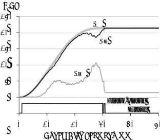
Bending mode Torsion mode Warp mode
The eight interpolation functions for eight-node solid element are:
1
( , , ) (1 )(1 )(1 ) 8
i i i
N x hz = +x x +h h +z zi (1)
with and where x, h and z are the
intrinsic coordinates of the element. Rewriting these interpolation functions in matrix form:
, , 1
i i i
x h z = ±
N[24×3],
interpolation of the velocity can be obtained: T u&=N U& (2) with x y z u u u é ù ê ú = ê ú ê ú ë û & & & & u and x y z U U U é ù ê ú = ê ê ú ë û & & & & U ú (3)
U& [24×1] is a vector of the nodal velocities and u&[3×1]
is the interpolated velocity field. Derivation of Equation (2) yields to the interpolation of the velocity gradient (expressed in vector form: L[9×1]).
T u N L U BU x x ¶ ¶ = = = ¶ 
& & &
(4)
where the velocity gradient interpolation matrix B[9×24] can be expressed in terms of the intrinsic
coordinates: 0
B= +B xBx+hBh+zBz +xhBxh+xzBxz+hzBhz (5) with sub-matrices B0[9×24] and Ba[9×24] (a=x, h, z,
xh, xz, hz) having the form of Equation (6), where bi[8×1] (i=x,y,z) are vectors constructed from the nodal
coordinates, while bia [8×1] vectors depend on the nodal
coordinates and are functions of the intrinsic coordinates x,h,z. 0 0 0 0 0 0 0 0 0 0 0 0 0 0 0 0 0 0 0 T x T y T z T x T y T z T x T y T z b b b b B b b b b b é ù ê ú ê ú ê ú ê ú ê ú ê ú ê ú = ê ú ê ú ê ú ê ú ê ú ê ú ê ú ê ú ê ú ë û , 0 0 0 0 0 0 0 0 0 0 0 0 0 0 0 0 0 T x T y T z T x T y T z T x T y T z b b b b B b b b b b a a a a a a a a a a é ù ê ê ê ê ê ú ê ú ê = ê ê ê ê ê ê ê ú ê ú ë û 0 ú ú ú ú ú ú ú ú ú ú ú (6)
FIGURE 1. Hourglass mode types
The BWD3D element is defined with only one integration point (IP). So, evaluation of the velocity gradient at the IP induces that the interpolation matrix
B reduces to B0, because the IP is located at the center
of the element (x=h=z=0). This consideration yields to
the existence of twelve non-zero deformation modes U& corresponding to a velocity gradient L equal to zero at the IP. These are the so-called hourglass modes: 6 bending modes, 3 torsion modes and 3 warp (non-physical) modes (see Fig. 1).
Stress computed at the IP corresponding to hourglass modes is zero (because L=0). Without particular care, the deformation energy associated to hourglass modes would be zero. No stiffness of the element with respect to hourglass deformation modes would derive.
Gratefully, an estimation of the stress field inside the element can be obtained using the tangent stiffness
matrix C[9×9] as shown by Equation (7), where s&[9×1]
is the stress field expressed in vector form, s&0 is the
stress at IP and &s , x s& , h s& , z s& , xh s& , xz s& are the hz
six so-called hourglass stresses. Note that, according to the FE time integration, the derivative of the stress with respect to time is actually computed.
0 0 CL C B Bx Bh Bz Bxh Bxz Bhz U x h z xh xz hz s x h z xh xz hz s xs hs zs xhs xzs hzs = é ù = ë + + + + + + û = + + + + + + & & & & & & & & &
(7)
With this stress field and the velocity gradient inside the element (Equation (4)), a non-zero deformation energy can be attributed to hourglass modes.
However, it is generally admitted that the energy computed thanks to the hourglass stresses is too high, depending on the deformation mode applied to the element. Consequently, the element is sometimes too stiff. This problem is known as locking phenomenon. A simple method used to avoid locking is to replace B
matrix by B[9×24] matrix:
0
Where B0 is identical as in Equation (5), while the
Ba[9×24] (a=x, h, z, xh, xz, hz) matrices have the
form of Equation (9), where e1, e2 and e3 are
parameters used to avoid volumetric locking, i.e. locking problem occurring during volumetric
deformation. Parameter b is introduced to reduce shear
locking (linked to shear strains).
1 3 2 2 1 3 3 2 1 0 0 0 0 0 0 0 0 0 0 0 0 T T T x y z T y T z T x T T T x y z T z T x T y T T T x y z e b e b e b b b b B e b e b e b b b b e b e b e b a a a a a a a a a a a a a b b b b b b é ê ê ê ê ê ê ê = ê ê ú ê ú ê ú ê ú ê ú ê êë a a a ù ú ú ú ú ú ú ú ú ú úû (9)
The volumetric locking can be completely eliminated by choosing e1=2/3 and e2=e3=-1/3.
Unfortunately, the shear locking cannot be treated as simply. The value of b (Î[0,1]) should be adapted to the deformation mode applied to the element: a value near 0 is recommended for bending dominated problems to avoid shear locking while a value around 1 should be used during shearing of the element to avoid hourglass modes without deformation energy.
The main drawbacks of the shear locking method proposed by Equations (8) and (9) are the dependence of the optimum b-value on the deformation undergone by the element. To facilitate the determination of b, some authors propose to approximate the deformation mode dependence by a dependence on the element shape [10,11]. A second drawback is the non-objectivity of the B matrix, i.e. dependence of the element behavior on the global reference axes. This second drawback can hardly be avoided.
These considerations led us to the development of a new locking treatment method: the Wang-Wagoner method [9], implemented in the BWD3D element. To do so, Equations (4) and (5) are adapted in order to be expressed in term of hourglass modes:
3 1 2 4 1 2 3 4 T T T T T i j i j j j j j u h h h h b x x g x g x g x g æ ¶ = +¶ +¶ +¶ +¶ çç ¶ è ¶ ¶ ¶ ¶ & & U ö ÷÷ ø (10) with h1=hz;h2 =xz;h3 =xh;h4 =xhz
In equation (10), the first term in parenthesis corresponds to uniform shear (if i¹j) or uniform tension (if i=j), while
g
1[8×1],g
2[8×1],g
3[8×1],g
4[8×1] arelinked to four hourglass modes: two bending modes, one torsion mode and one warp mode (the twelve hourglass modes are recovered for i=1,2,3).
According to [9], locking problems can be avoided by eliminating adequate hourglass modes. For shear locking, the uniform shear and the hourglass torsion modes must be kept while the two bending and the warp modes are identified to be at the origin of shear locking; therefore, they should be eliminated. Equation (10) is modified into Equation (11) for i¹j:
T T i i j i i j j u h b x x g æ ö ¶ = + ¶ çç ¶ è ¶ ø & & U ÷÷ (i¹j; no sum on i) (11) To prevent volumetric locking, Equation (10) becomes Equation (12) in order to eliminate the dilatational strain caused by torsion, bending and warp hourglass modes. 4 4 4 4 4 4 2 3 1 1 3 3 T T T T i k l j k l i j j j j T T T T T T i l i k k l i l i k k k k l l l u h h h b U x x x x h h h h h h U U x x x x x x g g g g g g g g g æ é ùö ¶ =ç + ê¶ +¶ +¶ ú÷ ç ÷ ¶ è êë¶ ¶ ¶ úûø æ¶ ¶ ¶ ö æ¶ ¶ ¶ - çç¶ +¶ +¶ ÷÷ - çç¶ +¶ +¶ è ø è & & & ö÷÷& ø 3 (12) (i= j; i¹ ¹k l; i k l, , =1, 2, ; no sum on i,k,l) In order to be able to identify the hourglass modes (which is a crucial point of the method), Equation (10) must be expressed in a corotational reference system [8], closely linked to the element coordinates. This reference system must have its origin at the center of the element and its reference axes are aligned (as much as possible, depending on the element shape) with element edges. A grateful consequence of this corotational reference system is a simple and accurate treatment of the hourglass stress objectivity, by using initial and final time step rotation matrices.
The shear locking and the volumetric locking method proposed by Equations (11) and (12) associated with the corotational reference system has been successfully implemented in the BWD3D element of LAGAMINE FE code. The Wang-Wagoner method, contrarily to the method using a bparameter (Equation (9)), has deep physical roots, which makes it very efficient for various FE analyses. Up to now, the BWD3D element has proved its superiority (compared with elements having a shear locking treatment using a
b parameter) during deep drawing simulations,
HARDENING MODELS
Teodosiu and Hu’s hardening model is described by 13 material parameters:
p R Sd SL X L P 0 Sat sat
C , C , C , C , C , f , n , n , r, Y , R , S , X0 (13)
and depends on four state variables:
P,S, X, R (14) Variable P is a second order-tensor that depicts the
polarity of the persistent dislocation structures (PDSs in [1]) and S is a fourth-order tensor that describes the directional strength of the PDSs. Scalar R represents the isotropic hardening due to randomly distributed dislocations and the second-order tensor X is the back stress. These state variables evolve with respect to the plastic strain rate ep and the equivalent plastic strain rate
& p& with the form:
( )
pY
Y& =f Y,e& & (15) p
A precise description of these evolution equations can be found in [5,12]. It should however be noticed that the fourth-order tensor S must be decomposed into SD the strength of the dislocation structure associated
with the currently active slip systems and SL, the part
of S associated with the latent slip systems, according to Equation (16).
L D
S=S Ne&pÄNe&p+S (16) where Ne&p is the plastic strain rate direction. Two
distinct evolution equations are applied to SD and SL.
Yield condition is given by Equation (17).
y Y0 R f | S
s s= = + + | (17)
where s is the equivalent stress, function of dev( ) Xs - , is the current elastic limit, is the initial size of the yield locus and
y
s Y0
R+f | S| represents the evolution of the isotropic hardening. The expression of s depends on the definition of the yield locus.
The implementation of Teodosiu and Hu’s hardening model into one FE code is not straightforward [4]. Equation (15), describing the evolution of the state variables, must be adapted to be introduced in FE codes, due to the discretization of the
time evolution. A particular attention has been paid to the evolution rule for S. During monotonic loading,
Ne&p is constant and the decomposition of S thanks to Equation (16) yields to a SL-value remaining equal to
zero, if initially zero. For smooth strain path changes, Ne&p evolves continuously and therefore SL should
neither be activated (different opinions concerning this point can be found in literature). Contrarily, for an abrupt strain-path change, Ne&p varies discontinuously and SL is activated. When implemented in FE codes,
without particular care, during continuous evolution of Ne&p, SL would be activated due to the evolution of
Ne&p-value from one time step to the next one. Different numerical solutions can be investigated. In this study, the method proposed by Alves [12,13] and Balan using the plastic strain rate direction at the end of the step for the decomposition of S was compared with Hoferlin’s method [1,14] using Ne&p at the beginning of the step.
Furthermore, the classical isotropic Swift hardening was also used. The formulation is:
(18)
(
y C 0 p
n
s = e +
)
where p is the accumulated equivalent plastic strain, while C,e0 and n are material parameters.
DEEP DRAWING SIMULATIONS
The deep drawing process proposed by [1] was investigated in the present study. It consisted of an axisymmetric deep drawing process with a punch having a flat bottom. The diameter of the blank was 100mm, the punch diameter was 50mm (the drawing ratio was then 2.0), the punch fillet radius was 5mm, the matrix opening was 52.5mm and the matrix fillet radius was 10mm. The blankholder force was prescribed to 12 kN. The Coulomb friction coefficient between the blank and the tools was m=0.10 according to experimental lubrication technique.TABLE 1. Hardening Parameters of the IF Steel.
Model Parameters
Swift C=530.4 MPa, e0=0.00159, n=0.2596 Teodosiu CP=3.3, CR=26.94, CSD=5.35, CSL=13.45,
CX=24.98, f=0.6, nL=1.88, nP=27.1, r=3.93, Y0=114.9 MPa, Rsat=78.4 MPa,
FIGURE 2. Earing profile for Minty constitutive law, with and without texture evolution; experimental results from [1].
2
1
0
FIGURE 3. Earing profile obtained by [1] and with Hill 1948 law; experimental results from [1].
The material used was an interstitial-free (IF) steel with a thickness of 0.8mm. Thanks to X-ray measurements, it appeared that the initial texture of this IF steel presented a strong g-fiber, typical of rolled steel sheets. The hardening parameters of this steel are summarized in Table 1. Due to the orthotropy of the IF steel, only a quarter of the process was studied. The steel sheet was meshed with one layer of 531 BWD3D elements. The tools were meshed with triangular foundation facets.
As the whole steel sheet was swallowed during the punch travel, the earing profile was measured as the cup height versus the angle from rolling direction (RD). Figure 2 presents the earing profile computed with the micro-macro Minty constitutive law [2]. The computation of texture evolution has been activated (curves called “Evol”) or not, i.e. the initial texture was used throughout the simulation (curves “Minty”). The influence of the hardening behavior was also analyzed. Swift type isotropic hardening was used (curves “Swift”) and the mixed hardening of Teodosiu
presented above was also tested (curves “Teo”). The Hill 1948 yield locus was also investigated for the deep drawing simulation. Figure 3 presents the earing profile obtained with the Hill law coupled with Swift and Teodosiu hardening models. Experimental values and results obtained by [1] (with a texture based law and isotropic and kinematic hardening models) are also plotted for comparison purpose.
0 0.5 1 1.5 2 0 15 30 45 60 75 9
Angle from Rolling Direction (°)
Ear ing ( mm) Minty_Swift Minty_Teo Evol_Swift Evol_Teo Experiment
According to Fig. 2, it appears that the influence of the hardening behavior on the earing profile was negligible when texture was not updated. This is consistent with the results of [1]. These models are indeed very similar: they are both based on Taylor’s model using initial texture, coupled with identical Swift (isotropic) and Teodosiu (mixed) hardening models. The main difference is the definition of the yield locus (see [2] and [1]).
0 0.5 1.5 2.5 3 0 15 30 45 60 75 90
Angle from Rolling Direction (°)
Earing (mm) Tex-Iso Tex-Mic Hill_Swift Hill_Teo Experiment from [1]
When texture evolution was computed throughout the simulation, a large effect of the hardening model was noticed. A shift of the minimum value from 45° to 40° and a significant asymmetry of the earing profile appeared when Teodosiu’s hardening model was used, which was confirmed experimentally. The results obtained with Hill law show a too large amplitude of the earing profile. The influence of the hardening model is almost not existent in these curves. According to the earing profile prediction, the micro-macro constitutive law with computation of texture evolution coupled with Teodosiu’s hardening model yielded best results.
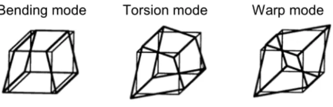
The evolutions of particular Teodosiu’s hardening variables are shown on Figs. 4 and 5 for the two tested methods used to implement Teodosiu’s hardening model in the FE code: Hoferlin’s one and Alves-Balan’s one. One particular element along RD was chosen such that it underwent completely the bending and unbending linked to the deep drawing process. Even if we have checked it had negligible effects on the earing profile, the implementation method appeared to have significant influence on the evolution of the directional strength of the PDSs, described by fourth-order tensor S. Evolution of the norm of SL, the
latent part of S, began soon in the simulation with Alves-Balan’s method: the first maximum around punch displacement 14mm corresponds to the bending of the steel sheet, while the second maximum around 27mm appeared during the unbending. Contrarily, Hoferlin’s method required elastic-plastic transition for the activation of SL, which only appeared after the
unbending. The end of the simulation was characterized, for the selected element, by a translation with low strains; this elastic state yielded to constant hardening values.
0
FIGURE 4. Evolution of Teodosiu’s hardening variables with Hoferlin’s method.
0
FIGURE 5. Evolution of Teodosiu’s hardening variables with Alves-Balan’s method.
CONCLUSIONS
The new BWD3D element with its improved shear locking treatment allowed to obtain accurate FE results, as shown by the deep drawing process investigated in the present study. The effect of texture evolution and hardening model were assessed through earing profile prediction. The hardening model used (Swift and Teodosiu) appeared to have almost no effect on earing profile if the yield locus shape remained constant during the simulation. Contrarily, when texture evolution was computed, a large effect of hardening model was noticed. The combination of Teodosiu’s hardening model and texture evolution yielded very good results. The method used to implement Teodosiu’s model in FE code was also analyzed. It had no effect on the earing profile
prediction while very different hardening variable evolutions were observed. The question about which implementation method is preferable is still open.
-50 50 100 150 200 250 0 10 20 30 40 5 Punch Displacement (mm) (MPa) ½S½ SD
ACKNOWLEDGMENTS
A. M. Habraken is mandated by the National Fund for Scientific Research (Belgium). The authors thank the Belgian Federal Science Policy Office (Contract P5/08) for its financial support.
½SL½
Elasto-plastic Elastic
0
REFERENCES
1. Li, S., Hoferlin, E., Van Bael, A., Van Houtte, P., Teodosiu, C., Int. J. Plast. 19, 647-674 (2003).
-50 50 100 150 200 250 0 10 20 30 40 5 Punch Displacement (mm) (MPa)
2. Habraken, A.M., Duchêne, L., Int. J. Plast. 20, 1525-1560 (2004).
½S½
3. Teodosiu, C., Hu, Z., “Evolution of the intragranular microstructure at moderate and large strains: modeling and computational significance” in Proc. NUMIFORM, edited by Shen, S.F. and Dawson, P.R., pp. 173-182.
SD
4. Hiwatashi, S., Van Bael, A., Van Houtte, P., Teodosiu, C., Comput. Materials Science 9, 274-284 (1997).
½SL½
5. Bouvier, S., Alves, J.L., Oliveira, M.C., Menezes, L.F.,
Comp. Mater. Sci. 32, 301-315 (2005).
6. Castagne, S., Pascon, F., Bles, G., Habraken, A.M., J. de
Physique IV 120, 447-455 (2004). Elasto-plastic
Elastic 7. Habraken, A.M., Cescotto, S., Int. J. Numerical Methods
in Engineering 30, 1503-1525 (1990).
0 8. Belytschko, T., Bindeman, L. P., Comput. Methods Appl. Mech. Engrg. 88, 311-340 (1991).
9. Wang, J., Wagoner, R. H., “A New Hexahedral Solid Element for 3D FEM Simulation of Sheet Metal Forming” in Proc. NUMIFORM, edited by Ghosh, S. et al., AIP Conf. Proc. 712, 2004, pp. 2181-2186.
10. Li, K. P., Cescotto, S., Comput. Methods Appl. Mech.
Engrg. 141, 157-204 (1997).
11. Alves de Sousa, R. J., Cardoso, R. P. R., Fontes Valente, R. A., Yoon, J.-W., Gracio, J. J., Jorge, R. M. N., “Development of a One Point Quadrature EAS Solid-Shell Element” in Proc. NUMIFORM, edited by Ghosh, S. et al., AIP Conf. Proc. 712, 2004, pp. 2228-2233. 12. Alves, J.L., Oliveira, M.C., Menezes, L.F., “An
advanced constitutive model in sheet metal forming simulation: the Teodosiu microstructural model and the Cazacu Barlat yield criterion” in Proc. NUMIFORM, edited by Ghosh, S. et al., AIP Conf. Proc. 712, 2004, pp. 1645-1650.
13. Alves, J.L., Simulação Numérica do Processo de estampagem de chapas metálicas Modelação Mecância e Métodos Numéricos, Ph. D. Thesis, University of Minho (2003).
14. Hoferlin, E., Incorporation of an accurate model of texture and strain-path induced anisotropy in simulations of sheet metal forming, Ph. D. Thesis, Katholieke Universiteit Leuven, 2001.
![FIGURE 2. Earing profile for Minty constitutive law, with and without texture evolution; experimental results from [1]](https://thumb-eu.123doks.com/thumbv2/123doknet/5646123.136631/5.918.107.443.101.335/figure-earing-profile-constitutive-texture-evolution-experimental-results.webp)