Multiplexage par division modale pour les applications à courte distance

(1)

Multiplexage par Division Modale pour les Applications

à Courte Distance

Thèse

Reza Mirzaei Nejad

Doctorat en Génie Électrique

Philosophiæ doctor (Ph.D.)

Québec, Canada

(2)

(3)

iii

Résumé

Le multiplexage par division de mode (MDM) a reçu une attention considérable de la part des chercheurs au cours des dernières années. La principale motivation derrière l'utilisation de différents modes de fibre optique est d'augmenter la capacité des réseaux de transport. Les expériences initiales ont montré une grande complexité dans le traitement de signal (DSP) du récepteur. Dans cette thèse, nous étudions la viabilité et les défis de la transmission de données sur des fibres à quelques modes (FMF) pour des systèmes MDM à complexité de DSP réduite. Nos études comprennent à la fois une transmission de données cohérente et non cohérente.

Dans notre première contribution, nous démontrons, pour la première fois, la transmission de données sur 4 canaux dans une nouvelle fibre OAM sans démultiplexage de polarisation optique. Nous utilisons une complexité de DSP réduite: deux jeux d'égaliseurs MIMO (multiple-input multiple-output) 2 × 2 au lieu d'un bloc égaliseur MIMO 4 × 4 complet. Nous proposons un nouveau démultiplexeur de mode permettant de recevoir simultanément deux polarisations d'un mode et de réaliser électriquement un démultiplexage de polarisation dans le récepteur DSP. Nous étudions également la pénalité OSNR due aux imperfections dans le démultiplexeur de mode et nous examinons la vitesse de transmission maximum accessible pour notre système.

Dans notre deuxième contribution, nous étudions les dégradations modales dans les systèmes OAM-MDM, en nous concentrant sur leur effet sur la performance et la complexité du récepteur. Dans notre étude expérimentale, nous discutons pour la première fois de l'impact de deux modes non porteurs de données sur les canaux de données véhiculés par les modes OAM. Deux types différents de fibres OAM sont étudiés. Nous caractérisons notre liaison MDM en utilisant les techniques de mesure du temps de vol et de réponse impulsionnelle. Nous discutons des conclusions des résultats de caractérisation en étudiant l'impact des interactions modales sur la complexité de l'égaliseur du récepteur pour différents scénarios de transmission de données.

Dans le troisième chapitre, nous étudions un nouveau FMF à maintien de polarisation et conduisons deux séries d'expériences de transmission de données cohérentes et de radio sur fibre (RoF). Nous démontrons pour la première fois, la transmission de données sans MIMO sur six et quatre canaux dans les systèmes cohérents et RoF, respectivement. Nous démontrons également, pour la première fois, la transmission de données RoF sur deux polarisations d'un mode dans une FMF. Nous discutons de la dégradation des performances due à la diaphonie dans de tels systèmes. Nous étudions également l'impact de la courbure sur cette fibre dans un contexte de RoF. La propriété de maintien de polarisation de cette fibre sous courbure est étudiée à la fois par des expériences de caractérisation et de transmission de données.

(4)

(5)

v

Abstract

Mode division multiplexing (MDM) has received extensive attention by researchers in the last few years. The main motivation behind using different modes of optical fiber is to increase the capacity of transport networks. Initial experiments showed high complexity in DSP of the receiver. In this thesis, we investigate the viability and challenges for data transmission over specially designed few mode fibers (FMF) for MDM systems with reduced DSP. Our studies include both coherent and non-coherent data transmission.

In our first contribution, we demonstrate, for the first time, data transmission over 4 channels in a novel OAM fiber without optical polarization demultiplexing. We use reduced DSP complexity: two sets of 2×2 multiple-input multiple-output (MIMO) equalizers instead of a full 4×4 MIMO equalizer block. We propose a novel mode demultiplexer enabling us to receive two polarizations of a mode simultaneously and conducting polarization demultiplexing electrically in receiver DSP. We also investigate the OSNR penalty due to imperfections in the mode demultiplexer and we examine the maximum reachable baud rate for our system.

In our second contribution, we study the modal impairments in OAM-MDM systems, focusing on their effect on receiver performance and complexity. In our experimental study, for the first time, we discuss the impact of two non-data carrying modes on data channels carried by OAM modes. Two different types of OAM fibers are studied. We characterize our MDM link using time-of-flight and impulse response measurement techniques. We discuss conclusions from characterization results with studies of the impact of modal interactions on receiver equalizer complexity for different data transmission scenarios .

In the third contribution, we study a novel polarization-maintaining FMF and conduct two sets of coherent data transmission and non-coherent radio over fiber (RoF) experiments. We demonstrate for the first time, MIMO –Free data transmission over six and four channels in coherent and RoF systems, respectively. We also demonstrate, for the first time, RoF data transmission over two polarizations of a mode in a FMF. We discuss the performance degradation due to crosstalk in such systems. We also study the impact of bending on this fiber in RoF context. The polarization maintaining property of this fiber under bending is studied both via characterization and data transmission experiments.

(6)

(7)

vii

List of Tables

Table 3.1. Crosstalk measurement for each mode group ... 33 Table 4.1. Measured DMGD between OAM0 and OAM1 mode groups per fiber ... 46 Table 4.2. Measured crosstalk (dB) among OAM modes in OAM-MDM link for 1.47 km RCF and 1.1 km IPGIF ... 51 Table 4.3. Summary of parameters in characterization and data transmission related to memory depth of equalizers ... 58 Table 5.1. Measured effective index separation between data carrying vector modes ... 66 Table 5.2. Received modal power matrix for coherent data transmission over 6 vector modes in (dB); columns are transmitted modes and rows are received modes ... 69 Table 5.3. Received modal power matrix at RF carrier of 3.3 GHz for bending radius of 4.5 cm in (dB); columns are transmitted modes and rows are received modes ... 74 Table 5.4. Received modal power matrix at RF carrier of 3.3 GHz for bending radius of 4.5 cm in (dB); columns are transmitted modes and rows are received modes ... 79

(11)

(12)

xii

List of Figures

Fig. 1.1. Time line for bit rate increase of optical transmission systems with different

technologies ... 2

Fig. 1.2. Different physical technologies to create orthogonal signal sets ... 3

Fig. 1.3. The key components of a MDM transmission system ... 5

Fig. 1.4. Butterfly Equalizer structure for Polarization demultiplexing ... 7

Fig. 1.5. PDM systems with (a) optical polarization demultiplexing (b) electrical polarization demultiplexing ... 8

Fig. 1.6. MIMO equalizer structure for a 6×6 MDM system ... 10

Fig. 1.7. Equalizer block for an MDM system supporting D/2 modes in two polarizations with separate mode detection ... 12

Fig. 2.1. DSP Blocks of a single mode single polarization system ... 17

Fig. 2.2. DSP blocks for a single mode dual polarization system ... 20

Fig. 2.3. DSP blocks for a non-coherent OFDM systems in (a) transmitter (b) receiver. .... 21

Fig. 3.1. OAM-MDM data transmission setup ... 29

Fig. 3.2. (a) Setup for free-space OAM mux and demultiplexer stages, (b) spiral phase patterns for OAM±1 at SLM of mux stage, (c) blazed forked gratings for OAM±1 at SLM of demultiplexer stage ... 30

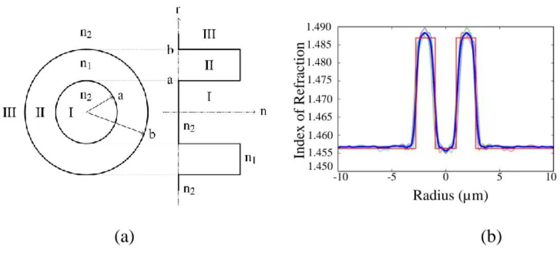
Fig. 3.3. (a) Cross section of RCF fiber, (b) Designed (red) and measured index profile (blue: averaged, others: x- and y-scan on both directions) ... 32

Fig. 3.4. BER vs. OSNR for all four data channel ... 34

Fig. 3.5. OSNR penalty vs. crosstalk from OAM0 on OAM1 mode group ... 35

Fig. 3.6. BER vs. baud rate for all four data channels ... 36

Fig. 4.1. (a) Channel model for interactions among vector modes propagating in OAM fibers supporting modes of order zero and one. Fiber output when launching a pulse in 4 supported vector modes (b) assuming no interaction among modes (c) with interactions among modes ... 43

Fig. 4.2. Setup for Time of flight measurement ... 46

Fig. 4.3. ToF measurement results, (a) IPGIF (b) RCF ... 47

Fig. 4.4. OAM-MDM characterization and data transmission setup ... 47

Fig. 4.5. Channel impulse response for OAM-MDM link using a 1.47 km RCF with scales of (dB) and (ns) on x and y axes of sub figures. ... 48

Fig. 4.6. Channel impulse response for OAM-MDM link using a 1.2 km IPGIF with scales of (dB) and (ns) on x and y axes of sub figures. ... 49

Fig. 4.7. Enlarged channel impulse response for case of sending and receiving OAM +1 in (a) 1.2 km IPGIF (b) 1.47km and 450 m RCF ... 50

(13)

xiii

Fig. 4.8. BER at OSNR = 16 dB vs. number of taps, (a) sending only OAM0, (b) sending

only OAM±1; Length of IPGIF and RCF are 1.2km and 1.47 km, respectively. ... 55

Fig. 4.9. BER at OSNR = 25 dB vs. number of taps, sending all modes and (a) detecting OAM0, (b) detecting OAM±1; Length of IPGIF and RCF are 1.2km and 1.47 km, respectively. ... 56

Fig. 4.10. BER vs number of taps for OAM±1 channels, RCF fibers of 1.47 km at OSNR=25 dB and 450 m at OSNR=16 dB ... 57

Fig. 5.1. Experimental setup for MIMO–Free 6 channels QPSK data transmission over PM-ERCF ... 67

Fig. 5.2. BER versus OSNR for six channels data transmission over PM-ERCF at 24 Gbaud ... 70

Fig. 5.3. RoF over PM-ERCF data transmission setup ... 71

Fig. 5.4. Crosstalk versus RF carrier frequency for each mode channel ... 73

Fig. 5.5. BER versus received power at RF carrier of 2.4 GHz ... 75

Fig. 5.6. BER versus received power at RF carrier of 3.3 GHz ... 76

Fig. 5.7. BER versus received power at RF carrier of 3.3 GHz for LPV11b,y channel when transmitting various combinations of channels; insets are measured crosstalk on LPV11b,y ... 76

Fig. 5.8. Loss and crosstalk measurement versus fiber spool bending at RF carrier of 2.4 GHz ... 79

Fig. 5.9. Crosstalk on channels versus RF carrier frequency with bending fiber of radius 4.5 cm added to the main spool ... 80

Fig. 5.10. BER vs received power for sending two polarizations of LPV11b with bending applied to the fiber at RF carrier of 2.4 GHz ... 81

(14)

(15)

xv

Abbreviations

AWG Arbitrary Wave Generator

B2B Back-to-Back

BER Bit Error Rate

BPG Bit Pattern Generator

BS Beam Splitter

CD Chromatic Dispersion

CP Cyclic Prefix

CPR Carrier Phase Recovery

CW Continuous-Wave

DAC Digital-to-Analog Converter

DD Decision Directed

DDO-OFDM Direct-Detection Optical Orthogonal Frequency-Division Multiplexing

DP Dual Polarization

DSP Digital Signal Processing

EDFA Erbium-Doped Fiber Amplifier

EVM Error Vector Magnitude

FEC Forward Error Correction

FFT Fast Fourier Transform

FIR Finite Impulse Response

FOR Frequency Offset Estimation

IFFT Inverse Fast Fourier Transform

IR Impulse Response

ISI Inter-Symbol Interference

(16)

xvi

LO Local Oscillator

LP Linearly Polarized

LPF Low-Pass Filter

LW Line-Width

MDM Mode Division Multiplexing

M-QAM M-Ary Quadrature amplitude modulation

MIMO Multiple-input multiple-output

MMSE Minimum mean square error

MZM Mach-Zehnder modulator

NRZ Non-return-to-zero

OAM Orbital Angular Momentum

OBPF Optical band pass filter

OFDM Orthogonal frequency-division multiplexing

OSA Optical Spectrum Analyzer

OSNR Optical signal-to-noise ratio

P/S Parallel-to-serial

PBC Polarization beam combiner

PBS Polarization Beam Splitter

PC Polarization controller

PD Photo-Detector

PDM Polarization-division multiplexing

PMD Polarization Mode Dispersion

PRBS Pseudorandom binary sequence

QAM Quadrature Amplitude Modulation

QPSK Quadrature phase-shift keying

(17)

xvii

RTO Real-time oscilloscope

S/P Serial-to-parallel

SDM Space Division Multiplexing

SE Spectral efficiency

SMF Single-mode fiber

TDM Time-division multiplexing

ToF Time of Flight

VOA Variable optical attenuator

(18)

(19)

xix

List of Symbols

m Modulation order

n Number of bits per symbol

ti Transmitted signal in ith_channel

ri Received signal in ith_channel

τi Differential mode group delay of mode i

D Number of modes used in system

Ri Fourier transform of the received signal in ith_channel

Ti Fourier transform of the transmitted signal in ith_channel

Hij Channel transfer function for sending channel i and receiving channel j

uij Equalizer output for sending polarization i and receiving polarization j

Vi Equalizer output for polarization i

wij Equalizer filter coefficients for case of sending channel i and receiving channel j

L Number of taps of equalizer

Δ Step of convergence for equalization algorithm

ε Error function in equalization algorithm tap update

(20)

(21)

xxi

To my parents, Esfandyar and Mah Monir

(22)

(23)

xxiii

Acknowledgment

I would like to express my sincere gratitude to my director, Professor Leslie A. Rusch, for all she taught me during my Ph.D. studies. For a project with extensive experimental studies, I faced many challenges but I never felt alone in this way and always had her support and help. I admire the considerable amount of time she spent with me going step by step through different phases of this project. I do appreciate her guidance, kindness and patience throughout my studies during these years.

I would also like to thank Prof. Sophie LaRochelle, member of COPL, who has been involved in this project and helped me wherever possible.

Next, I would like to thank the post docs with who I spent a lot of my time in the laboratory: Dr. Pravin Vaity for invaluable efforts to build the free space optics setup for mode multiplexer and demultiplexer and running the initial experiments with me; Dr. Karen Allahverdyan who committedly came to laboratory with me every single day including weekends. A special thanks to Dr. Lixian Wang who helped me after Karen left our group. His enthusiasm for academic research is admirable. I would also like to thank Farzan Tavakoli who helped me in the last few months of the experiments.

I had the chance to find many good friends at COPL who were part of my life here. I would like to thank Hadi, Siamak, Amin, Hassan, Bahareh, Alessandro, Charles, Gabriel and Omid for the good times we spent together.

Last but not least, I would like to thank my family who always encouraged me to pursue my studies and always supported me during all these long years that I have been in academia.

(24)

(25)

xxv

Foreword

Three chapters of this thesis are based on materials published in conference and journal papers. Most of the contents in these three chapters are the same as the journal papers; however, some modifications are made to the introduction of chapters and some supportive material are added for better coherence. I was the main contributor to these papers

Chapter 3: Reza Mirzaei Nejad, Karen Allahverdyan, Pravin Vaity, Siamak

Amiralizadeh, Charles Brunet, Younès Messaddeq, Sophie LaRochelle, and Leslie Ann Rusch, “Mode Division Multiplexing Using Orbital Angular Momentum Modes Over 1.4-km Ring Core Fiber,” Journal of Lightwave Technology, vol. 34, no. 18, Sept. 2016.

This paper demonstrates for the first time, data transmission over four channels using OAM modes of order zero and one with reduced DSP complexity. Two sets of 2×2 equalizer blocks were used instead of a full 4×4 MIMO equalizer. We used, for the first time, electrical polarization demultiplexing in OAM-MDM systems. Karen Allahverdyan and Pravin Vaity helped me with the free space optics setup. Siamak Amiralizadeh helped me with optical signal to noise ratio sweeping. Charles Brunet designed the fiber used in the experiment. Younès Messaddeq and Sophie Larochelle gave guidance for fiber design and fabrication. Leslie A. Rusch guided and managed the whole project including fiber design, building the setup and data transmission experiments. I built and ran the data transmission setup; debugged and completed the offline DSP; helped with the finalizing the free space setup and having a clear alignment routine. I wrote the paper and it was revised by the co-authors.

Chapter 4: Reza Mirzaei Nejad, Lixian Wang, Jiachuan Lin, Sophie LaRochelle, and

Leslie A. Rusch, “The impact of Modal Impairments on Receiver Complexity in OAM Fibers,” Journal of Lightwave Technology, vol. 35, no. 21, Nov. 2017.

(26)

xxvi

This paper discusses the modal impairments observed during OAM fiber characterization and how these impairments affect receiver complexity and the performance of the equalizer block. Lixian Wang helped me with the free space optics setup and fiber characterization. Jiachuan Lin helped me with the data transmission. Sophie LaRochelle advised us on characterization techniques. The project was led by Leslie A. Rusch. I did the experiments and analyzed the results in the discussions section. I chose the characterization techniques required; completed measurements and analyzed results from data transmission. I wrote the paper and it was revised by the co-authors.

Chapter 5: Reza Mirzaei Nejad, Farzan Tavakoli, Lixian Wang, Xun Guan, Sophie

LaRochelle, and Leslie A. Rusch, “RoF Data Transmission using Four Linearly Polarized Vector Modes of a Polarization Maintaining Elliptical Ring Core Fiber,” submitted to Journal of Lightwave Technology. Lixian Wang, Reza Mirzaei Nejad, Alessandro Corsi, Jiachuan Lin, Younès Messaddeq, Leslie Rusch, and Sophie Larochelle, “Linearly polarized vector modes: enabling MIMO-free mode-division multiplexing,” Optics Express, vol. 25, no. 10, pp.11736-11748, May 2017.

For the first paper, Farzan Tavakoli and Lixian Wang helped with building the free space optics setup. Xun Guan provided me with his DSP code for narrowband OFDM transmission and reception. I built and ran the data transmission setup. I also proposed the ideas for performance evaluation in RoF context and investigating the bending characteristic and polarization maintaining properties of the fiber using data transmission results. I wrote the paper and it was revised by the co-authors.

I was the second author of the second paper. I did the data transmission experiment. The sections describing the data transmission setup and the performance evaluation results are extracted from this paper and discussed and compared with the results of first paper of this chapter in the thesis.

(27)

(28)

1

Chapter 1

Introduction

1.1. Capacity crunch in optical transport network

The amount of traffic carried by optical transport networks has increased rapidly over the last decades. In the past two decades, and due to new telecom and Datacom services, a growth of around 30 to 60% per year in different geographic regions was observed [1], [2]. New applications, which require higher bandwidth, are being introduced every day. The number of users for different services, from digital media to mobile applications is increasing annually and will require more and more bandwidth in fiber optics backbone networks [3], [4]. In this section, we first review the technologies that have helped to increase the capacity of optical transport networks over the past decades. Next, we discuss the solutions to increase capacity in future networks.

The timeline of bit rate increase in optical transmission systems with different technologies is shown in Fig. 1.1. For over two decades, the bit rate increase was achieved via wavelength-division multiplexed (WDM) optical transmission systems [5]. This was itself mainly accomplished by improvements in optoelectronic device technologies. For

(29)

2

example, by introduction of lasers that could reach GHz frequency stability and optical filters that would let the engineers exploit 50 GHz frequency grids, the capacity was further increased.

After developments in physical technologies leading to better and more sophisticated devices, in the next phase, the telecommunication techniques played a significant role to increase the spectral efficiency by sending more information in the same bandwidth provided by optical devices. In the last decade, we have observed the adoption of many concepts from wireless communications in optical communications. This includes several techniques such as i) higher order modulation formats, i.e., quadrature amplitude modulation (QAM) accompanied with coherent detection instead of simply a non-coherent on-off keying modulation, ii) different digital signal processing (DSP) techniques and also iii) error correction coding [6-9].

Fig. 1.1. Time line for bit rate increase of optical transmission systems with different technologies [10]

While the single mode optical fiber transmission systems are reaching their capacity limit imposed by the combination of Shannon’s information capacity limit and nonlinear fiber effects [11], the demand for higher capacity is still increasing annually. Considering this issue, alternative techniques are required to support the amount of traffic foreseen for future networks.

(30)

3

In Fig. 1.2, all the physical dimensions in an optical fiber that can be used to create orthogonal signal sets for either modulation or multiplexing are illustrated.

Fig. 1.2. Different physical technologies to create orthogonal signal sets [10]

In what follows, we briefly review them:

I) The quadrature dimension which is the in-phase and quadrature components of the signal, are used to create higher order modulation formats, i.e. quadrature amplitude modulation (mQAM) formats where the number of bits per symbol, n, is increased by the order of modulation, m, following the expression n = log m bits ₂

per symbol. As the modulation order is increased, system performance will be more sensitive to noises and impairments of optical links, resulting in system performance degradation and imposing a restriction to using high spectral efficiency when a certain bit error rate (BER) is required.

II) The frequency dimension is used for multiplexing different data channels to different wavelengths in WDM systems. The capacity is scaled by the number of frequency channels used by the system. However, WDM related impairments, as

(31)

4

well as the available frequency band and the bandwidth of optical components used in the transmission link, limit the arbitrary increase in number of frequency channels.

III) The polarization dimension is used for polarization-division multiplexing (PDM). It can give a two-fold increase in capacity by sending two data streams on two orthogonal polarization states of the fundamental mode propagating in single mode fiber.

IV) The time dimension is used for multiplexing where different time slots are assigned to different channels to create a time division multiplexing (TDM) system. This technique clearly cannot increase the capacity of the network but it can be used as a way to share the same channel between different users.

V) The space dimension uses different modes of fiber as independent data channels to increase the capacity scaled by the number of modes exploited. Since the number of modes supported by fibers can be infinite in theory, there is a huge interest in studying the possibilities of space division multiplexing (SDM) or mode division multiplexing (MDM) as the main candidate for capacity increase in future networks. We will discuss MDM systems in more detail in the next section.

1.2. Mode division multiplexing

In MDM, different modes out of an orthogonal modal basis are chosen as independent data channels. Exploiting more than one mode, and combining the idea of MDM with currently available WDM systems, can significantly increase the capacity of transport networks. The conceptual diagram for the key components in MDM system is shown in Fig. 1.3, where ti

(32)

5 Mo d e Mu lti p le xe r Mo d e D e M u lti p le xe r Multimode Amplifier Few Mode Fiber

D in p u t, D o u tp u t Eq u al iz er Receiver DSP

...

t

1

t

2

t

D

r

1

r

2

r

D

Fig. 1.3. The key components of a MDM transmission system

The key components in MDM systems include modal multiplexer /demultiplexer, few mode fiber (FMF) and multimode amplifiers. For mode (de)multiplexing, different techniques and devices have been used such as phase plates [12], spatial phase modulators [13] or photonic lanterns [14]. New fibers are being developed for MDM systems supporting different number of modes [15]. Research on multimode amplifiers that could amplify the modes supported by the MDM system with the same gain value is another important research area [16] that can lead to a fundamental improvement in reach and capacity of MDM systems.

Although MDM systems can increase the capacity of transport networks, they suffer from modal impairments that can affect the performance or complexity of the receiver. The two main impairments in the linear regime in MDM systems include modal coupling and modal dispersion. With a well-designed fiber, modal coupling, i.e., crosstalk, can still occur in an MDM link due to various reasons such as fiber imperfection, non-ideal mode multiplexer and demultiplexer or mechanical stresses such as bending and twisting. Modal dispersion or differential mode group delay (DMGD) occurs as different modes have different group velocities and therefore, they travel with different speeds in the fiber. If D independent signals are launched at the transmitter on D modes simultaneously, they arrive at the receiver in different times with different group delays (GD), τi, i =1, 2, .. D.

DSP in MDM systems is used to compensate the modal impairments. They key block to compensate the modal impairments is the equalizer block. In general, for a system using D channels, an equalizer block with D inputs and D outputs is required. DMGD among different modes can affect the memory depth requirement of equalizers.

(33)

6

Depending on the strength of modal coupling among different modes, MDM systems can be divided to two groups of “strong” and “weak” mode coupling. In general, the level of modal crosstalk can affect the required dimension of the equalizer block. The equalizer block complexity, for these two groups of systems are different. In next section, we will discuss the structure and complexity of the equalizer block for MDM systems in strong and weak coupling regimes.

1.3. Equalizer complexity in MDM systems

An equalizer block in the receiver DSP of coherent detection systems is responsible for correcting the impairments introduced by the channel and the devices used at the transmitter and receiver side of the system [17]. One important task of equalizer for systems using more than one polarization of one mode is to undo the coupling between different polarization channels. In next sections, we first discuss the structure of equalizer for the current single-mode, commercial PDM systems, and then we discuss the generalization to MDM systems and the ensuing challenges.

1.3.1. Polarization demultiplexing in single mode dual polarization

systems

PDM systems use two polarizations of the fundamental mode as two independent data channels. Signals on the two polarization ( X and Y) mix with each other during fiber propagation. The channel interactions can be described in the frequency domain in matrix form as 1 11 12 1 2 21 22 2

( )

R

H

T

R

H

T





 







 





 



(1.1)

(34)

7

where R1, R2, T1 and T2 are the received and transmitted signals in two polarizations of X and Y, respectively at frequency . This is the transfer function, also called the Jones matrix, representation where Hij indicates the channel frequency response when sending polarization i and receiving polarization j. To recover the signal in each of the polarizations, we need an equalizer block that implements the inverse of the channel frequency response.

The equalizer block should receive the two polarization tributaries simultaneously to compensate for the polarization related impairments such as polarization mixing and polarization mode dispersion (PMD). The signals received in two polarizations are equalized using the so-called butterfly equalizer structure shown in Fig. 1.4, where wij are vectors of the time domain filter taps of the equalizer to recover the desired signal for polarization j from the received signal in polarization i. These taps are the inverse Fourier transform of the frequency response in the Jones matrix, and uij indicates the equalizer

output where the input is from polarization i to recover the data in polarization j.

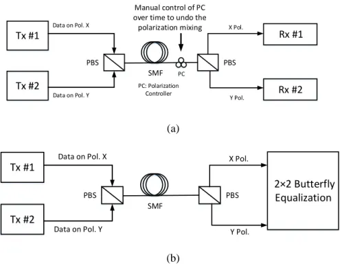
For short reach applications, where PMD is negligible, it is possible to use a polarization controller on the fiber and undo the polarization mixing optically. By using this method, we do not need the butterfly equalizer structure. However, this method requires constant manual intervention to adjust the paddles of polarization controller to undo the time varying polarization mixing. Modern communications system use more practical electrical polarization demultiplexing in the DSP of receiver. Fig. 1.5 compares these two methods.

w12 w21 w22 w11 Received data in Pol. X Received data in Pol. Y Equalized data in Pol. X Equalized data in Pol. Y 2 ×2 Eq u al iz er uxx uyx uxy uyy r1 r2 Vx Vy

(35)

8 Tx #1 Tx #2 Data on Pol. X Data on Pol. Y PBS PBS SMF PC X Pol. Y Pol. PC: Polarization Controller Manual control of PC over time to undo the polarization mixing Rx #2 Rx #1 (a) Tx #1 Tx #2 2×2 Butterfly Equalization Data on Pol. X Data on Pol. Y PBS PBS SMF X Pol. Y Pol. (b)

Fig. 1.5. PDM systems with (a) optical polarization demultiplexing (b) electrical polarization demultiplexing

1.3.2. Equalizer blocks in multi-mode dual polarization systems

For a system that supports transmission of D/2 modes in two polarizations carrying D data channels, in general an equalizer block with D inputs and D outputs is required. The task of the equalizer block is to compensate for the modal impairments including modal mixing, i.e. crosstalk, and modal dispersion. In the following, we will discuss the structure of the equalizer block for strong and weak modal coupling regimes.

Mathematically, the transfer function can be described by Eq. (1.2) where Ti and Ri are

the transmitted and received signals in the frequency domain for the ith_channel,

respectively. The channel frequency response is Hij when sending channel (a particular

polarization and mode) i and receiving channel j. In the next sections, we discuss the regimes of strong and weak coupling.

(36)

9 1 11 1 1 1

( )

.

( )

.

( )

.

( )

D D D DD D

T

H

R

T

H

R





 





 





 





 



 





 





 





 





 



(1.2)

1.3.2.1. Strong mode coupling regime

In this regime, modes of different order fully mix during propagation. All the elements Hij of the channel frequency response matrix are non-zero. To recover the data in each of D channels, a DD equalizer block (full MIMO equalizer) should be used to receive and

process the data in all D channels simultaneously. The equalizer block should find the inverse of the channel frequency response. As an example, an equalizer block for a 66 MDM system is shown in Fig. 1.6 [10]. Here ri and ui are the received data and equalized data, for channel i, respectively, and wij represents theequalizer taps in the time domain to recover the desired signal for channel j from the received signal in channel i.

1.3.2.2. Weak mode coupling regime

In this case, interactions between modes of different order are low; the only strong modal interaction is the polarization mixing. The channel matrix can be regarded as a matrix with zero, or very small, elements that are of the main diagonal and its nearest diagonal on either side. The diagonal 2×2 submatrices represent the polarization mixing within a mode. The transfer function can be described as (1.3)

(37)

10 r1 r2 r3 r4 r5 r6 u1 u2 u3 u4 u5 u6 R ec e iv ed d at a in ch an n el # 1 R ec e iv ed d at a in ch an n el # 2 R ec e iv ed d at a in ch an n el # 3 R ec e iv ed d at a in ch an n el # 4 R ec e iv ed d at a in ch an n el # 5 R ec e iv ed d at a in ch an n el # 6 Recovered data in channel #6 Recovered data in channel #5 Recovered data in channel #4 Recovered data in channel #3 Reccovered data in channel #2 Recovered data in channel #1

Fig. 1.6. MIMO equalizer structure for a 6×6 MDM system, [10]

11 12 21 22 1, 1 , 1 1, , ( ) ( ) 0 .. 0 ( ) ( ) . . . . . . . . ( ) ( ) 0 . . ( ) ( ) D D D D D D D D H H H H H H H H                              _ _  _ _  _ _   (1.3)

For sufficiently weak mode coupling, each mode can be detected independently. In practice, this can be achieved by designing specialty fibers with effective indices of

(38)

11

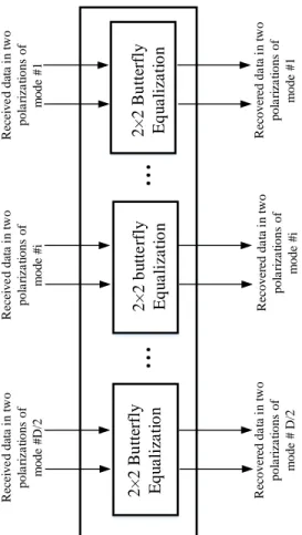
different modes that are sufficiently separated for minimum modal crosstalk. Given two polarizations per mode are used as data transmitting channels, an equalizer block similar to Fig. 1.4 could be used per mode in such systems. Instead of a large equalizer block covering all channels, we will have D/2 blocks of 2×2 equalizers. These 2×2 equalizers are used to compensate only for polarization mixing within each of the modes. It should be noted that if the polarizations of the modes do not mix with each other, i.e., if they are polarization maintaining, then we simply need D equalizers for D channels, i.e., a diagonal matrix. The structure of equalizer for such systems is shown in Fig. 1.7.

1.3.2.3. Equalizer complexity comparison between strong and weak

mode coupling regimes

As explained in section 1.3.2.1, systems working in the strong coupling regime require full MIMO equalizers. In systems using D/2 modesand two polarizations per mode, it includes simultaneous reception of D channels and MIMO processing with D×D equalizer blocks, i.e., D2_{equalizers in total. In general, the size of the equalizer block increases with the}

square of the number of channels. For example, demonstrations using 3 and 15 modes with two polarizations were reported in [18], [19]. For these systems, equalizers with dimension of 6×6 and 30×30 were used, requiring 36 and 900 equalizers in total, respectively. Such equalizer structures can be prohibitively complex for real time realization of receiver DSP in terms of size and power consumptions. The reported demonstrations were using offline DSP processing. Since fabricating fibers for strong coupling regime is less challenging, most of the early MDM transmission demonstrations were in strong coupling regime.

In recent years, researchers are focusing on decreasing the DSP complexity of MDM systems. The main solution is to design fibers and MDM links for separate mode detection, i.e., the weak coupling regime. For systems with separate mode detection, the number of equalizers is linearly related to the number of channels used. Comparing the increase of complexity of equalizers in these two regimes show the advantage and importance of separate mode detection. However, designing fibers and establishing an optical link with low modal mixing is quite challenging.

(39)

12

...

2 × 2 b u tt e rfl y E q u a li za ti o n 2 × 2 Bu tt erfl y E q u a li za ti o n 2 × 2 Bu tt erfl y E q u a li za ti o n R ec ei ve d da ta i n t w o pol a ri za ti ons of m ode # 1 R ec ei ve d da ta i n t w o pol a ri za ti ons of m ode # i R ec ei ve d d at a i n t w o pol a ri za ti ons of m ode # D /2 R ec ove re d da ta i n t w o pol a ri za ti ons of m ode # 1 R ec ove re d d a ta i n t w o po la ri za ti on s o f m ode # i R ec ove re d da ta i n t w o pol a ri za ti ons of m ode # D /2

Fig. 1.7. Equalizer block for an MDM system supporting D/2 modes in two polarizations with separate mode detection

1.4. Thesis structure

The motivation behind this project is to study and demonstrate the viability of low complexity MDM systems. The capacity is increased by a multiplicative factor equal to the number of modes, but the complexity is less than the full MIMO processing. For this purpose, different fiber designs are characterized and used in data transmission experiments. In the following, we describe the structure of the thesis.

In chapter 2 we give a brief overview of the electrical digital signal processing used in the characterization and transmission experiments reported in the thesis.

In chapter 3, we discuss data transmission demonstration over an OAM fiber supporting four channels. The experimental setup for data transmission and mode multiplexer and

(40)

13

demultiplexer setup with free space optics components is described in detail. The performance evaluation is presented via BER performance versus optical signal to noise (OSNR) ratio, and BER versus baud rate for high OSNR. The performance penalty due to crosstalk is also discussed. The two main contributions in this chapter include

i) Introducing a polarization diverse mode demultiplexer allowing electrical demultiplexing of the two polarizations of each mode.

ii) Transmitting four channels, for the first time, over an OAM fiber link of length 1.4 km.

In chapter 4, we discuss the modal impairments observed in OAM fibers and how they can affect the receiver complexity and in particular the memory depth of equalizers. Two different type of OAM fibers with different refractive index profiles are studied. The main contributions in this chapter include

i) Channel impulse response measurements for an OAM-MDM system are reported for the first time.

ii) For the first time, the impact of non-data-carrying modes of TE01 and TM01

on data carrying modes and equalizer memory depth is shown.

iii) The impact of parameters such as differential mode group delay (DMGD) and modal crosstalk on receiver performance and complexity in an OAM-MDM system is discussed based on two characterization techniques ( time-of-flight and channel impulse response measurements) and verified via data transmission results.

In chapter 5, data transmission results are reported for another type of fiber designed for separate mode detection. This fiber also benefits from a polarization maintaining property.

(41)

14

Two set of experiments are discussed for coherent detection and radio over fiber (RoF) non-coherent detection. The contributions of this chapter include

i) For the first time, we demonstrated data transmission over six vector mode of a polarization maintaining fiber in a coherent detection scheme. The receiver equalizer structure is even more simplified and instead of a 22 equalizer block for processing two polarizations of a mode simultaneously, a single equalizer per polarization of a mode is used.

ii) For the first time, we transmit four radio frequency (RF) signals over four linearly polarized vector modes. The impact of parameters such as RF carrier frequency and modal crosstalk are investigated.

iii) The impact of bending on fiber performance in terms of crosstalk changes and polarization maintaining property are discussed via characterization and data transmission results.

(42)

(43)

16

Chapter 2

DSP for MDM systems

2.1. Introduction

In this chapter, we present a very brief review of the structure of the DSP required for the receiver in coherent detection and non-coherent orthogonal frequency division multiplexing (OFDM) systems. We review the blocks for the coherent detection in 2.2. These techniques are used in experiments reported in chapters 3 and 4 and 5. The DSP blocks for non-coherent OFDM systems are reviewed in 2.3. These techniques are used in experiments reported in chapter 5.

2.2. DSP Blocks for Coherent Detection systems

In this section, we review the DSP blocks for coherent detection systems. We start with single-mode, single-polarization systems. We then discuss about the structure of DSP blocks for single-mode, dual-polarization systems.

2.2.1. DSP blocks in single-mode, single-polarization systems

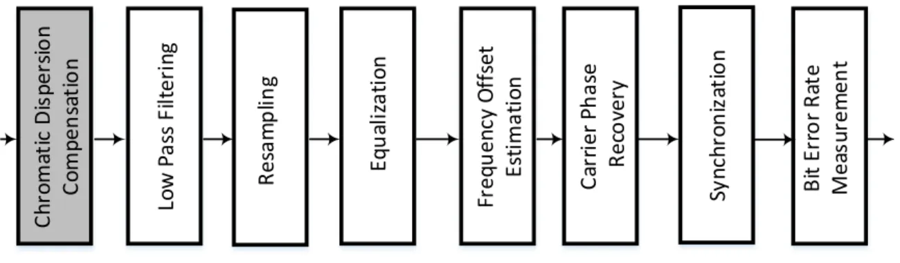
Essential DSP blocks for a conventional coherent detection system is shown in Fig. 2.1 Chromatic dispersion (CD) of the transmission link is compensated by digitally applying

(44)

17

the inverse of the CD transfer function of fiber in the frequency domain [20]. In this thesis, we do not use a block to compensate for CD. All our experiments are with short fibers of

C hr om at ic D is pe rs io n C om pe n sa ti o n Lo w P as s Fi lt er in g Eq u al iz at io n Fr eq u en cy O ff se t Es ti m at io n C ar ri er P h as e R ec o ver y B it E rr o r R at e M ea su re m en t Sy nc hr on iz at io n R es am p lin g

Fig. 2.1. DSP Blocks of a single mode single polarization system

around 1 km. The CD of a short link is negligible and this block is unnecessary for the short reach applications we target.

We low pass filter (LPF) to filter the out-of-band noise. We use a second order super Gaussian filter for this purpose. The bandwidth of the filter is set to 0.7×2× baud rate of the transmitted signal.

The next block is the resampling. The baud rate of the transmitted signal and the sampling rate of the real time oscilloscope (RTO) to capture the data in receiver side are not the same. The resampling block transforms captured data into a vector of received data with an arbitrary number of samples per symbol. This is achieved via interpolation techniques. We used two samples per symbol in our DSP.

Next we have a block for equalization. The equalizer is responsible for correcting the impairments introduced by channel and the devices used in transmitter and receiver side of a coherent detection system. These equalizers are the individual equalizers within the equalizer blocks discussed in chapter 2. The equalizer is realized by a finite impulse response (FIR) filter in the time domain with L taps. The filter coefficients can be found recursively using a steepest descent algorithm. The equalization algorithm could be blind or data aided. In a data-aided approach, the transmitted data is known at the receiver. The two major time domain adaptive algorithms widely used are constant modulus algorithm

(45)

18

(CMA) for blind adaptation and minimum mean square error (MMSE) algorithm for data-aided adaptation [21].

We used blind equalization, i.e., CMA, in all the experiments. The filter coefficients are updated by the expression

, 1 , *

,

1,2,...,

q k q k

k k q

w





w





r

_

q



L

(2.1)

where

w

q k, is the complex coefficient of the filter for the qth tap in the kth iteration of convergence, Δ is the step size (set at 10-4_{in our experiments), ε}

k is the error function and rk

is the kth_{received data sample. Complex conjugate of signal is denoted by *. The error}

function for CMA for phase shift keying (mPSK) modulation, is defined as

2

(1 |

| )

k

u

k

u

k







(2.2)

where uk is the equalizer output in the kth iteration [22]. The equalizer output, uk is calculated as

1 L k i k i i u w r_  



(2.4)

The next blocks are the frequency offset estimation (FOE) and carrier phase recovery (CPR) blocks. FOE is responsible for compensating the frequency drift between the transmitter and receiver lasers. We used mth power algorithm [23] for FOE which is mainly developed for mPSK modulations. m is the order of modulation, e.g. 4 for QPSK. In our experiments, we always used QPSK modulation, so the fourth power of the received complex signal is calculated. We find the peak in the resulting spectrum. The peak location in the frequency domain gives us the frequency offset between transmitter and receiver lasers.

CPR corrects for the laser phase drift at transmitter and receiver. We used the fourth power algorithm for phase noise correction in our CPR block [23]. This algorithm

(46)

19

calculates the phase drift by finding the angle of the fourth power of the received complex signal, thus removing the data modulation. For better accuracy, this procedure is done by assuming the phase drift is constant over multiple consecutive symbols. We find the angle of the average of fourth power of these symbols and remove it from the received data. We did the averaging over every eight symbols.

The next block is the synchronization block where the cross correlation between the received data and transmitted pseudo random binary sequence (PRBS) is calculated. The location of the peak in the cross correlation allows us to synchronize the received and transmitted data and thus count errors.

The final block is the BER measurement. We first assign the received symbols to the reference symbol in the QPSK constellation at the smallest Euclidean distance. We perform symbol to bit demapping and count errors by comparing the received bit sequence with the transmitted sequence.

2.2.2. DSP blocks in single-mode, dual-polarization systems

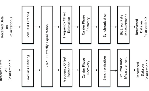
PDM systems use two polarizations of the fundamental mode as two independent data channels. The structure of the DSP block of such systems is also that of Fig. 2.1. There are two set of DSP blocks for each tributary at polarizations X and Y of the fiber, as seen in Fig. 2.2. The main difference with the single polarization system is the equalizer block where the equalizer taps of the two tributaries must be adapted simultaneously and jointly to compensate for the polarization related impairments.

The DSP blocks for PDM systems is shown in Fig. 2.2. The structure of the required 2×2 equalizer block was already discussed in section 1.3.1. Four filters coefficients are updated similar to (2.1), but with a significant difference. Here, the error signal is generated as the difference between the sum of the output of the two constituent equalizers per polarization and the transmitted data on the desired polarization. For example, the error function for the CMA algorithm for X polarization, using the same notation as Fig. 1.4., is defined as 2 , , , ,

(

)(1 |

| )

k

u

xx k

u

yx k

u

xx k

u

yx k











(2.5)

(47)

20

where uxx and uyx are the outputs of two equalizers in the butterfly structure in Fig. 1.4 with

inputs from received data in polarizations of X and Y used to recover the signal in X polarization; see Fig. 1.4.

Lo w P as s Fi lt er in g 2 ×2 B ut te rf ly E q ua liz at io n Fr eq u en cy O ff se t Es ti m at io n C ar ri er P h as e R ec o ve ry B it E rr o r R at e M ea su re m en t R ec ei ve d D at a o n Po la ri za ti o n X C ar ri er P h as e R ec o ver y B it E rr o r R at e M ea su rem en t Fr eq u en cy O ff se t Es ti m at io n Lo w P as s Fi lt er in g R ec ei ved D at a o n Po la ri za ti o n Y R ec o ve re d D at a o n P o la ri za ti o n X R ec o ve re d D at a o n P o la ri za ti o n Y Sy n ch ro n iz at io n Sy nc hr on iz at io n

(48)

21

2.3. DSP blocks for non-coherent OFDM systems

Sy n ch ro n iz at io n Se ri al t o P ar al le l c o n ve rs io n FF T Ze ro F o rc in g E q u al iz a ti o n Q A M d em o d u la ti o n & B ER

Fig. 2.3. DSP blocks for a non-coherent OFDM systems in (a) transmitter (b) receiver.

In our OFDM data transmission, the OFDM symbols are designed with parameters described in this section. A size 64 fast Fourier transform (FFT) is used, therefore, an OFDM symbol consists of 64 subcarriers in the frequency domain. Of these 64 subcarriers, there are 40 data-carrying subcarriers. Carrier spacing of the baseband OFDM signal is 10MHz. The cyclic prefix ratio of our OFDM symbol is 25%, appended to the beginning of the symbol. In a frame of 20 OFDM symbols, two symbols are used for training to estimate the channel. Subcarriers are modulated with 16 QAM modulation. The DSP blocks at the receiver for non-coherent OFDM systems in single-polarization, single-mode systems is shown in Fig. 2.4.

First, we synchronize the received data and the transmitted data, which is known to receiver. The synchronization block is realized by finding the largest peak in cross-correlation between the received and the transmitted data.

The next block is the serial to parallel formatting, and the removal of the CP. The FFT block converts the received data to the frequency domain.

The equalization block estimates the channel and equalize the received signal in frequency domain. The algorithm used in OFDM systems is the zero forcing algorithm [21], where each subcarrier of OFDM signal is equalized using a one-tap equalizer. We estimate the channel across all the subcarriers by using training symbols and comparing the received symbols with the transmitted ones in the frequency domain. Channel estimation is simply calculated for the two training OFDM symbols as

(49)

22 i i i R H T  (2.6)

where Ri and Ti are the received and transmitted symbols on the ith subcarrier; equalization is done over the 40 data-carrying subcarriers. The calculated values for Hi over the two OFDM symbols are averaged together for channel estimation.

The coefficients of the one-tap, zero-forcing equalizers are the inverse of the estimated channel responses. Since the DSP of OFDM is in frequency domain, the output of the equalizer is simply the product of the inverse of the channel and the input data to the equalizer block. Finally, the equalized QAM signal is de-mapped and BER is measured. We do the BER measurement in the same manner as coherent detection explained in section 2.2.1.

The size of the equalizer block for higher number of channels in MDM systems using non-coherent OFDM follows the same rules as those discussed in sections 1.3.2. The strong coupling regime requires a D×D zero forcing equalizer; in weak coupling regime, the signals can be recovered by 2×2 equalizers per mode. It should be noted that in case of polarization maintaining fibers working under weak coupling regime, the signals can be recovered using D duplicates of the DSP blocks for a single mode single polarization system with one equalizer per channel (Fig. 2.4).

(50)

(51)

24

Chapter 3

Mode Division Multiplexing using

Orbital Angular Momentum Modes over

1.4 km Ring Core Fiber

Résumé - Les systèmes de multiplexage en division modale (MDM) utilisant des modes de moment angulaire orbital (OAM) peuvent récupérer les données dans différents modes de traitement d'entrée duplex intégral (2D × 2D) - sortie multiple (MIMO). L'un des plus grands défis dans OAM-MDM est l’instabilité du mode suite à la propagation. Auparavant, la transmission de données OAM-MDM sans MIMO avec deux modes sur 1,1 km de fibre vortex a été démontrée lorsque le démultiplexage par polarisation optique était utilisé dans la configuration. Nous démontrons la transmission de données MDM en utilisant deux modes OAM sur 1,4 km d'une fibre à noyau annulaire (RCF) spécialement conçue sans utiliser le traitement MIMO complet ou le démultiplexage à polarisation optique. Nous démontrons l'importance du démultiplexage de polarisation, c'est-à-dire un MIMO minimal de 22, montrant la compatibilité de OAM-MDM avec des récepteurs de démultiplexage de polarisation de courant.

Abstract - Mode division multiplexing (MDM) systems using orbital angular momentum (OAM) modes can recover the data in D different modes without recourse to full (2D×2D) multiple input- multiple output (MIMO) processing. One of the biggest challenges in OAM-MDM systems is the modal instability following fiber propagation. Previously, MIMO-free OAM-MDM data transmission with two modes over 1.1 km of vortex fiber was demonstrated where optical polarization demultiplexing was employed in the setup. We demonstrate MDM data transmission using two OAM modes over 1.4 km of a specially designed ring core fiber (RCF) without using full MIMO processing or optical polarization demultiplexing. We demonstrate reception with electrical polarization demultiplexing, i.e.,

(52)

25

minimal 22 MIMO, showing the compatibility of OAM-MDM with current polarization demultiplexing receivers.

3.1. Introduction

As discussed in chapter 1, MDM systems have attracted much interest in recent years [24], [25] due to their ability to bypass the capacity limits of single mode systems. We discussed in detail the structure of equalizer block in MDM systems in section 1.4. Most of the demonstrated MDM systems using linear polarization (LP) modes over few mode fibers (FMF) [26] require full MIMO processing in receiver DSP [27]-[29].

Reducing receiver complexity in MDM systems is crucial for feasible real time operation, i.e., for reasonable processing speed and power consumption. Recently, a MIMO-free data transmission was reported over a 100 m graded-index ring core fiber [30]. Only mode groups were multiplexed (not individual modes) and there was no polarization division multiplexing (PDM), greatly reducing capacity. As coupling was negligible between mode groups, and there was no PDM, no MIMO was required. PDM combined with MDM offers highest capacity; but requires a 2×2 equalizer block for polarization demultiplexing for each mode. This is called dual polarization (DP)-MIMO.

Orbital angular momentum modes (OAM) [31] constitute an alternate modal basis for MDM systems. In this chapter, we focus on MDM data transmission systems. OAM-MDM systems offer the advantage of minimal mode coupling during propagation and thus reduced DSP complexity by eliminating the need for simultaneous detection of all modes and full MIMO processing. However, OAM modes cannot propagate in few mode fibers (FMF) designed for LP modes, but require specially designed fibers. One of the main challenges in OAM-MDM systems is mode instability at the optical fiber output after propagation.

OAM mode propagation was first demonstrated for 20 m and 900 m fibers [32], [33]. Successful MIMO-free OAM-MDM communications over 1.1 km of OAM fiber (called vortex fiber [34]), with simultaneous transmission of 4 channels over two OAM modes (order zero and one), was reported in [35], [36]. While MIMO-free, the transmission

(53)

26

scheme used optical polarization demultiplexing to undo the coupling between the two polarizations in each mode order.

In another experiment [37], successful data recovery without using MIMO processing was reported for OAM MDM data transmission system over 2 and 8 km conventional graded index multimode fiber. As in [30] for LP modes, neither PDM nor individual mode multiplexing was used, rather OAM mode groups (order zero to two) were exploited. Two data channels were constructed by choosing one mode out of degenerate modes inside mode groups of order zero to two (one channel from order zero, the other from order one or two) without polarization diversity.

In this chapter, we demonstrate successful data transmission over 1.4 km of ring core fiber (RCF) in four data channels of two OAM modes in two polarizations. For the first time, to the best of our knowledge, we use a polarization diverse demultiplexing scheme and successful data transmission is achieved without using full MIMO or manual optical polarization demultiplexing. We use electrical polarization demultiplexing in DSP, i.e., 2×2 equalizers for each mode group. We evaluate the BER performance versus OSNR. We examine the case of four channels data transmission and evaluate the OSNR penalty due to increasing the number of channels compared to single channel systems. Furthermore, we discuss the impact of crosstalk in mode demultiplexer and the resulting OSNR penalty.

The remaining sections of this chapter are organized as follows. In section 3.2, we discuss the principal of operation in OAM-MDM systems. In section 3.3, we describe the experimental setup used for data transmission and the details of our free-space, polarization-diverse OAM mux-demultiplexer stages. In section 3.4, we present results for crosstalk measurements in our OAM-MDM link. In section 3.5, we discuss the transmission experiment evaluating our OAM-MDM system performance. In section 3.6, we conclude the chapter.

3.2. Principles of Operation in OAM-MDM Systems

The motivation for using the OAM modal basis is to reduce the complexity of DSP in MDM systems. Complexity can be quantified via the number of equalizers required in

(54)

27

MDM reception. We consider only systems with full capacity where PDM is being combined with MDM, and all modes supported by the transmission system are used as distinct data channels. Therefore, this discussion will not include systems such as [30], [37], [38] where PDM is not used and only mode groups are used for data transmission. In general, for a LP-MDM system with D modes, we need full MIMO with a 2D×2D equalizer. The number of equalizers required in these LP-MDM systems with full MIMO processing scales with the square of the number of modes. Examples of this increase in complexity include LP-MDM systems (with two polarizations per mode) supporting 3 modes [28] and 15 modes [29], where equalizer blocks of 6×6 and 30×30 were used, respectively.

By using OAM modes, the complexity of DSP can be reduced, as the coupling between different modes can be low enough for separate mode detection. In OAM-MDM systems, the number of equalizers required scales linearly with the number of modes being exploited. As an example, and in our demonstration for a system using two OAM modes of OAM0 and OAM1 in two polarizations, supporting 4 data channels, two blocks of 2×2

equalizers (for polarization demultiplexing) are required instead of a 4×4 equalizer block.

We transmit simultaneously four data channels over two OAM modes. The order zero mode, the fundamental mode, is denoted by OAM0R and OAM0L where R and L denote

right and left circular polarization, respectively. The order one OAM modes are denoted by OAM+1 and OAM-1. The interactions between the two mode groups of order zero and one

are reduced to a minimum level by using specialty designed fibers for OAM modes propagation. The two polarizations of each of the two modes (zero and one) are degenerate leading to intra-mode coupling during propagation, i.e., OAM0L couples with OAM0R, and

OAM+1 couples with OAM-1. Hence, while MIMO processing of 4×4 equalizer can be

avoided, polarization demultiplexing on each mode group is required for successful data recovery in such systems.

Demultiplexing in [35], [36] used optical polarization demultiplexing using polarization controllers to separate the two polarizations of each mode rather than electronic separation. The demultiplexer setup was thus sequentially optimized for detection of each channel as they were captured; one polarization of one mode could be detected at a time at the

Multiplexage par division modale pour les applications à courte distance