CONDITIONAL HETEROSCEDASTICITY IN PACIFIC-BASIN
STOCK MARKET RETURNS
Corhay Albert, Tourani Rad Alireza
Abstract
This paper examines the statistical behavior of daily stock returns in several Pacific-Basin stock exchanges, which have grown tremendously in recent years. Empirical evidence reveals that return-generating models which empirically fit the data are processes with conditional heteroscedastic innovations. Particularly, the generalized autoregressive conditional heteroscedastic GARCH(1,1) process turns out to be the best in most cases.
Introduction
The purpose of this paper is to examine the empirical distribution of stock market returns in several Pacific-Basin stock exchanges and to find out which statistical model fits their distributions best. The distributional properties of stock returns have important implications for mean-variance portfolio theory, theoretical models of capital asset-pricing, and pricing of contingent claims. For instance, empirical tests of asset-pricing models and the efficient market hypothesis make statistical inferences based on distributional assumptions of stock returns, and estimation of the variance is essential in the Black-Scholes option-pricing formula.
The simplest and most practical assumption underlying the distribution of security returns is
multivariate normality with stationary parameters over time. As the normal distribution is stable under addition, any portfolio of stocks will also be normally distributed. If it is also assumed that investors are risk averse, mean-variance portfolio theory can be derived. Moreover, the assumptions of normality and parameter stability are implied by most of the statistical methods usually employed in empirical financial studies. Tests of normality hypothesis were first reported by Osborne (1964). He investigated returns of stock indices over several time periods and concluded they approximately follow normal processes. Other studies, however, questioned the normality assumption and showed that distributions of stock returns have fatter tails and are more peaked than the normal distribution. Mandelbrot (1963) and Fama (1965) observed that the family of stable Paretian distributions whose members exhibit heavy tails, conforms better to the distribution of stock returns.
Since then, there have been many models of stock returns describing processes that could generate distributions having heavier tails than normal distributions. For instance, Paretz (1972), and Blattberg and Gonedes (1974) showed that the scaled-f distribution, which can be derived as a continuous variance mixture of normal distributions, better fits daily stock returns than infinite variance stable Paretian distributions. Models using different mixtures of normal to generate distributions that would account for the higher magnitude of kurtosis, are, among others, the Poisson mixtures of Press (1967) and the discrete mixtures of Kon (1984). Furthermore, Clark (1973), Epps and Epps (1976), Merton (1982), and Tauchen and Pitts (1983) put forward models where the distribution of variance is a function of the arrival of the information rate, the trading activity, and the trading volume. Such models are, however, too complex to be used in empirical applications.
There is as yet no agreement regarding the best stochastic return-generating model. The general conclusion, however, seems to be that stock returns are approximately uncorrelated, but not
independent, and described by distributions with fatter tails. One of the most recently proposed class of return-generating process in the literature that can capture the temporal dependence of stock-return series is the class of autoregressive conditional heteroscedastic processes introduced by Engle (1982) and its generalized version by Bollerslev (1986). These processes allow for volatility clustering, that is, large changes are followed by large changes, and small by small, which has long been recognized as an important feature of stock-returns behavior. Empirical studies showed indeed that such processes are successful in modeling various time series (see, for example, French, Schwert, and Stambaugh 1987; Baillie and Bollerslev 1989; Hsieh 1989; Baillie and DeGennaro 1990).
In this paper, we show whether such models can adequately describe the stock-price behavior of Pacific-B asin capital markets. To that end, we have selected seven countries: Australia, Hong Kong, Japan, Korea, New Zealand, Singapore, and Thailand. The study of stock-price behavior in these
markets is interesting for it can provide further evidence in favor of or against the use of this type of model to describe stock-price behavior. The structure of the paper is as follows. The second section presents the data and the third section examines the statistical properties of the return series. In the fourth section, we apply an autoregressive model to the return series. The fifth section concerns the presentation and estimation of autoregressive conditional heteroscedastic processes. Conclusions follow in the last section.
The data
For this study, we selected the indices of seven stock markets in the Pacific-Basin rim. The daily market indices were collected from DATASTREAM for the period January 1, 1980 to September 30, 1990, and they are the All Ordinary Shares (Australia), the Hang Seng Index (Hong Kong), the Nikkei Down Jones (Japan), the Barclays Industrial (New Zealand), the Straits Times (Singapore), the Composite (South Korea), and the Bangkok Book Club (Thailand). The daily returns of these market indices are continuously compounded, they are calculated as the difference in logarithm of the index value for two consecutive days, Rt=log(Pt)-log(Pt-1).
Statistical analysis
This section contains a detailed analysis of the distributional and time-series properties of the stock-market-indices returns in the sample. A range of descriptive statistics are presented in Table 1, as well as the maximized likelihood function value when a normal distribution is imposed on data. The results confirm the well-known fact that daily stock returns are not normally distributed, but are leptokurtic and skewed, whatever the country concerned. All distributions are negatively highly skewed, indicating that they are nonsymmetric, and they all exhibit a high level of kurtosis, meaning they are more peaked and have fatter tails than normal distributions. In order to test the hypothesis whether returns are strict white noise, that is, random walk, the Box-Pierce test statistics up to lag 25 are calculated and presented in the table.
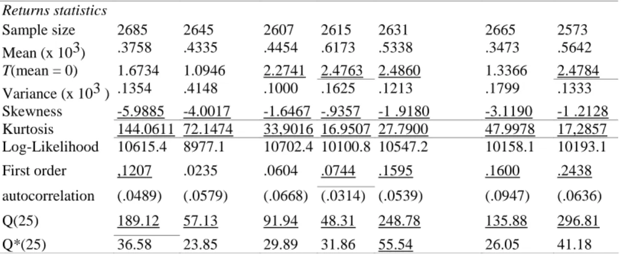
Table 1. Sample Statistics on Daily-Returns Series
Australia Hong Kong Japan Korea New Zealand I Singapore Thailand
Returns statistics Sample size 2685 2645 2607 2615 2631 2665 2573 Mean (x 103) .3758 .4335 .4454 .6173 .5338 .3473 .5642 T(mean = 0) 1.6734 1.0946 2.2741 2.4763 2.4860 1.3366 2.4784 Variance (x 103 ) .1354 .4148 .1000 .1625 .1213 .1799 .1333 Skewness -5.9885 -4.0017 -1.6467 -.9357 -1 .9180 -3.1190 -1 .2128 Kurtosis 144.0611 72.1474 33,9016 16.9507 27.7900 47.9978 17,2857 Log-Likelihood 10615.4 8977.1 10702.4 10100.8 10547.2 10158.1 10193.1 First order ,1207 .0235 .0604 .0744 .1595 .1600 .2438 autocorrelation (.0489) (.0579) (.0668) (.0314) (.0539) (.0947) (.0636) Q(25) 189.12 57.13 91.94 48.31 248.78 135.88 296.81 Q*(25) 36.58 23.85 29.89 31.86 55.54 26.05 41.18
Note: The tests statistically significant at the 5% level are underlined Numbers in parentheses are heteroscedasticity-consistent standard errors.
This is a joint test that the first k autocorrelation coefficients are zero. Under the null hypothesis, that the sample autocorrelations are not asymptotically correlated, the Box-Pierce statistic, Q = n ∑ik= ρ(i)2 has chi-square distribution with k degrees of freedom, where p(i) is the i-th autocorrelation. The values of Q are all significant at the 5% level for all countries. This implies that the null hypothesis of strict white noise is rejected, reflecting a rather long range of dependency in the returns series. However, it can be questioned whether this test accounts for the full probability distribution of the
returns series since heteroscedasticity can lead to the underestimation of the standard error, √1/n, of each sample, and therefore to the overestimation of the t- and chi-square statistics. Diebold (1987) provides a heteroscedasticity-consistent estimate of the standard error for the i-th sample
autocorrelation coefficient:
(1)
where γR2(i) is the i-th sample autocovariance of the square data and σ is the sample standard deviation of the data. These adjusted standard errors are presented in Table 1 under their respective autocorrelation coefficients. It can be seen that only four autocorrelation coefficients are statistically different from zero, whereas they are all significant, except that of Hong Kong, when√1/n is used as standard error.
Using the adjusted standard errors, Diebold proposed an adjusted Box-Pierce statistic:
(2)
which is asymptotically chi-square distributed with k degrees of freedom, under the null hypothesis of no serial correlation in the data. The values of Q* which are presented in Table 1 are much lower than the nonadjusted ones. They are significant at the 5% level for New Zealand only. So, even after adjusting for heteroscedasticity, there remains some significant long-term serial correlation in the series of returns for this country. A comparison between the values of Q and Q* suggests that the rejection of serial independence using Q, based on the standard testing procedure, is due to the presence of
heteroscedasticity in the returns series. However, the fact that the first lag autocorrelation is significant for six countries implies the rejection of white noise, that is, uncorrected process. Therefore, we have to eliminate the serial correlation in the return series before searching for appropriate models that could account for heteroscedasticity in the returns. One way to do this is to apply Autoregressive Moving Average (ARMA) models.
AUTOREGRESSIVE MODELS
The class of univariate ARMA models might adequately represent the behavior of the stock returns. In our case, an AR(1) model appears to fit returns series best.
(3)
The estimates of the above regression model for each country are presented in Table 2. In order to observe whether the residuals εt obtained from Equation (3) are uncorrected, we applied the same tests for normality and serial correlation as for the returns series. As before, the values of the autocorrelation coefficients and their respective standard errors adjusted for heteroscedasticity are presented in Table 2. The first order autocorrelation coefficient for all countries is not significantly different from zero, based on both adjusted and nonadjusted standard errors. The estimate of φi is statistically significant, except for Hong Kong. The Dickey-Fuller test for unit roots indicates that is significantly less than one. The series of returns appear to follow a stationary random walk. As far as the assumption of normality of the residuals is concerned, it can be rejected. The residual series appear to be leptokurtic and skewed. The comparison between values of Q and Q* is interesting in that while the former indicates significant serial correlation up to iag 25, the latter always rejects the presence of serial correlation. This shows that after controlling for heteroscedasticity, the AR(1) transformation of the returns provides an uncor-related series.
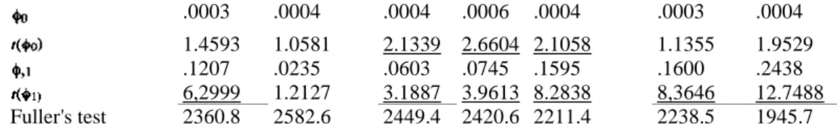
Table 2. The Autoregressive Model
Australia Hong Kong Japan Korea New Zealand Singapore Thailand
.0003 .0004 .0004 .0006 .0004 .0003 .0004 1.4593 1.0581 2.1339 2.6604 2.1058 1.1355 1.9529 .1207 .0235 .0603 .0745 .1595 .1600 .2438 6,2999 1.2127 3.1887 3.9613 8.2838 8,3646 12.7488 Fuller's test 2360.8 2582.6 2449.4 2420.6 2211.4 2238.5 1945.7 Residuals statistics
Mean (x 103) .0000 .0000 .0000 .0000 .0000 .0000 .0000 t(mean = 0) .0000 .0000 .0000 .0000 .0000 .0000 .0000 Variance (x 103 ) .1335 .4147 .0997 .1500 .1182 .1754 .1254 Skewness -5.7520 -.39343 -1.4590 .0687 -1.4676 -2,3729 -.7438 Kurtosis 140.3135 69.6704 34.1775 4,8406 25,9706 44.7506 16.6906 First order .0045 .0004 .0055 .0186 -.0015 -.0107 -.0119 autocorrelation (.0621) (.0599) (.0717) (.0316) (.0628) (.1061) (.0602) Q(25) 136.35 54.98 83.19 40.13 126.73 40.96 85.75 Q*(25) 27.24 23.31 28.97 30.41 30.74 17.20 18.48
Note: Statistical tests significant at the 5% level are underlined. Numbers in parentheses are heteroscedasticity-consistent standard errors.
Thus, it can be concluded that the residuals series is uncorrelated, but still exhibit heteroscedasticity.
Conditional heteroscedastic models
Various models have been developed to account for the presence of heteroscedasticity in stock-returns and market models (see Morgan 1976; Giaccoto and Ali 1982). While these models concentrate on unconditional heteroscedasticity, we use Engle's Autoregressive Conditional Heteroscedastic (ARCH) model, which focuses on conditional volatility movements. It is interesting to note that, according to Diebold, Im, and Lee (1988), the presence of ARCH effect appears to be generally independent of unconditional heteroscedasticity. Excess kurtosis observed in both returns and residuals series can be related to conditional heteroscedasticity, that is, its presence can be due to a time-varying pattern of the volatility. ARCH models and its extensions have been successfully applied, for instance, in foreign exchange markets by Baillie and Bollerslev (1989) and Hsieh (1989), and in stock markets by Akgiray (1989) and Baillie and De Gennaro (1990). The ARCH process imposes an autoregressive structure on the conditional variance which permits volatility shocks to persist over time. In this process, the conditional error distribution is normal, with a conditional variance that is a linear function of past squared innovations. The model, denoted by ARCH(p), is the following:
(4)
with p > 0; αi > 0, i = 0,..., p, and where Ω, is the information set of all information through time t, and the εt are obtained from a linear regression model. An important extension of the ARCH model is the Generalized Autoregressive Conditional Heteroscedasticity (GARCH) process of Bollerslev (1986), denoted by GARCH(p.q). In this model, the linear function of the conditional variance includes lagged conditional variances as well. Equation (4) in the case of a GARCH model becomes:
(5) where also q ≥ 0 and βj≥ 0,j=1,. .., q.
Before estimating (G)ARCH models, it is useful to test for the presence of ARCH properties on the returns series. This is the object of the next subsection.
Testing for ARCH Presence
In an ARCH process, the variance of a time series depends on past squared residuals of the process. Therefore, the appropriateness of an ARCH model can be tested by means of a LM test, that is, by
regressing the squared residuals against a constant and lagged squared residuals (Engle 1982).
(6)
Under the null hypothesis of no ARCH process, the coefficient of determination R2 can be used to obtain the test statistic TR2 which is distributed as a chi-square with i degrees of freedom. This LM test has been applied to our series up to lag 5 for all the seven returns series. The values we obtained for the TR2 are reported in Table 3.
Table 3. LM Test Statistic
Lags Australia Hong Kong Japan Korea New Zealand Singapore Thailand
ARCH (1) 30.32 73.09 369.74 461.78 378.13 1065.21 617.39
ARCH (2) 32.48 73.11 373.98 480.38 381.33 1068.83 654.98
ARCH (3) 49.81 76.75 407.92 486.51 396.53 1087.83 809.87
ARCH (4) 55.64 76.69 408.53 486.69 590.12 1090.96 813.77
ARCH (5) 61.34 76.85 411.58 490.91 591.99 1104.42 819.67
Note: A11 LM test statistics for ARCH (p) are significant at the 1% level.
They are all statistically significant at the 1% level, which strongly indicates the presence of an ARCH process in the series.
Estimating (G)ARCH Models
The parameters of a (G)ARCH model are obtained through a maximum likelihood estimation. Given the return series and initial values of el and hl for l=0,..., r and with r = max(p,q), the log-likelihood function we have to maximize for a normal distribution is the following:
(7)
where T is the number of observations; ht, the conditional variance, is defined by Equations (4) and (5) for the ARCH and GARCH models respectively; and εt2 are the residuals obtained from the appropriate linear regression model according to the country in consideration.
As the values of p and q have to be prespecified in the model, we tested several combinations of p and q. The values of the maximized likelihood functions for all pairs of p and q are presented in Table 4. We also calculated the generalized likelihood ratioof the maximized likelihood functions under the null hypothesis, that is, the normal distribution, and the various alternate hypothesis. Under the null hypothesisLRis chi-square distributed with degrees of freedom equal to the difference in the number of parameters under the two hypotheses. Table 4 gives the values of the LR test for each model. It can be observed that the value of the LR test for all (G)ARCH models is statistically significant at the 1% level, which means that all of these models are more likely to fit the data than is the normal distribution. In order to distinguish between an
improvement in the likelihood function due to a better fit and an improvement due to an increase in the
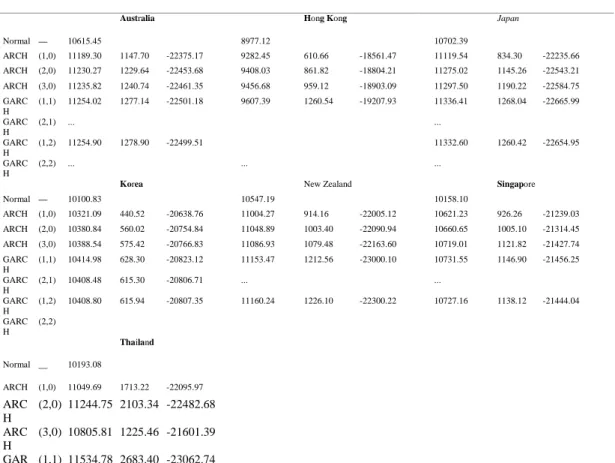
order-selection criterion, where K is the number of parameters in the model. Table 4. Maximum Log Likelihoods for (G)ARCH Models
Model p,q Log Likelihood
LRTest Schwarz Criterion Log Likelihood LRTest Schwarz Criterion Log Likelihood LR Test Schwarz Criterion
Australia Hong Kong Japan
Normal — 10615.45 8977.12 10702.39 ARCH (1,0) 11189.30 1147.70 -22375.17 9282.45 610.66 -18561.47 11119.54 834.30 -22235.66 ARCH (2,0) 11230.27 1229.64 -22453.68 9408.03 861.82 -18804.21 11275.02 1145.26 -22543.21 ARCH (3,0) 11235.82 1240.74 -22461.35 9456.68 959.12 -18903.09 11297.50 1190.22 -22584.75 GARC H (1,1) 11254.02 1277.14 -22501.18 9607.39 1260.54 -19207.93 11336.41 1268.04 -22665.99 GARC H (2,1) ... ... GARC H (1,2) 11254.90 1278.90 -22499.51 11332.60 1260.42 -22654.95 GARC H (2,2) ... ... ...
Korea New Zealand Singapore
Normal — 10100.83 10547.19 10158.10 ARCH (1,0) 10321.09 440.52 -20638.76 11004.27 914.16 -22005.12 10621.23 926.26 -21239.03 ARCH (2,0) 10380.84 560.02 -20754.84 11048.89 1003.40 -22090.94 10660.65 1005.10 -21314.45 ARCH (3,0) 10388.54 575.42 -20766.83 11086.93 1079.48 -22163.60 10719.01 1121.82 -21427.74 GARC H (1,1) 10414.98 628.30 -20823.12 11153.47 1212.56 -23000.10 10731.55 1146.90 -21456.25 GARC H (2,1) 10408.48 615.30 -20806.71 ... ... GARC H (1,2) 10408.80 615.94 -20807.35 11160.24 1226.10 -22300.22 10727.16 1138.12 -21444.04 GARC H (2,2) Thailand Normal __ 10193.08 ARCH (1,0) 11049.69 1713.22 -22095.97 ARC H (2,0) 11244.75 2103.34 -22482.68 ARC H (3,0) 10805.81 1225.46 -21601.39 GAR (1,1) 11534.78 2683.40 -23062.74
CH GAR CH (2,1) ... GAR CH (1,2) 11529.41 2672.66 -23048.59 GAR CH (2,2) ...
Note: ... indicates where the optimization routine failed.
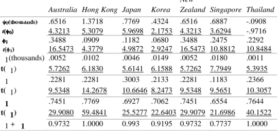
Table 5. Model Estimates
New
Australia Hong Kong Japan Korea Zealand Singapore Thailand
.6516 1.3718 .7769 .4324 .6516 .6887 -.0908 4.3213 5.3079 5.9698 2.1753 4.3213 3.6294 -.9716 .3488 .0909 .1182 .0680 .3488 .2475 .2292 16.5473 4.3779 4.9872 2.9247 16.5473 10.8812 10.8484 α1(thousands) .0052 .0102 .0046 .0149 .0052 .0180 .0011 t(α1) 5.7262 6.1830 5.6141 6.1588 5.7262 7.7949 5.3935 α1 .2281 .2281 .3003 .2133 .2281 .1183 .2366 t(α1) 9.5348 14.2678 10.6646 8.2473 9.5348 9.5651 10.3057 β1 .7451 .7769 .6927 .7062 .7451 .6554 .7644 t(β1) 29.9080 59.4841 25.5277 22.6403 29.9079 21.6986 40.1522 α1 + β1 0.9732 1.0000 0.993 0.9195 0.9732 0.7737 1.0000
Note: t-statistics significant at the 5% level arc underlined.
According to this criterion, the model with the lowest SIC value fits the data best. The SIC values are reported in Table 4. The GARCH(1,1) model has the lowest SIC values for all countries. Table 5 contains the results of the model best fitting the series of returns for each country. The sum ofin the conditional variance equations measures the persistence of the volatility. Engle (1982) and Bollerslev (1986) have shown that if this sum is equal to one, the GARCH process becomes an integrated GARCH or IGARCH process. Such an integrated model implies the persistence of a forecast of the conditional variance over all future horizons and also an infinite variance of the unconditional distribution of εt. Therefore, a restricted test on the sum of the parameters must be carried out. We calculated the sum of
the parameters for the appropriate (G) ARCH models. They are respectively 0.9732, 0.993, 0.9195, 0.9732, and 0.7737 for Australia, Japan, Korea, New Zealand, and Singapore. They are less than unity, though rather close to one for most of them, which indicates a long persistence of shocks in volatility. As for Hong Kong and Thailand, the sum of the α1 and β1 was greater than one. This indicates that the series are not stationary and an integrated model is more appropriate, that is, the conditional variance follows an integrated process. The IGARCH(1,1) model has therefore been
estimated for these two countries.
Conclusions
This paper examines the return properties of seven Pacific-Basin stock markets. It provides empirical support that the class of autoregressive conditional hetero-scedasticity models is generally consistent with the stochastic behavior of daily stock returns. Descriptive statistics and normality tests reveal that the distribution of returns is not normal, whatever the country concerned. It has further been shown that the residuals obtained after applying an AR(1) model, which accounts for the presence of first-order autocorrelation in the returns, exhibit nonnormality and heteroscedasticity. Then we tested various models belonging to the class of autoregressive conditional heteroscedasticity models. Among them the GARCH(1,1) fits the data best for Australia, Japan, Korea, New Zealand, and Singapore, and the IGARCH(1,1) for Hong Kong and Thailand.
References
Akgiray, V. (1989). "Conditional Heteroscedasticity in Time Series of Stock Returns: Evidence and Forecasts." Journal of Business 62: 55-80.
Baillie, R.T. and T. Bollerslev (1989). "The Message in Daily Exchange Rates: A Conditional-Variance Tale." Journal of Business & Economic Statistics 7: 297-305.
Baillie, R.T. and R.P. De Gennaro (1990). "Stock Returns and Volatility." Journal of Financial and Quantitative Analysis 25: 203-214.
Black, F. and M. Scholes (1973). "The Pricing of Options and Corporate Liabilities." Journal of PoliticalEconomy 81: 637-654.
Blattberg, R.C. and N.J. Gonedes (1974). "A Comparison of the Stable and Student Distribution of Statistical Models for Stock Prices." Journal of Business 47: 244-280.
Bollerslev, T. (1986). "Generalized Autoregressive Conditional Heteroskedasticity." Journal of Econometrics 31: 307-327.
Clark, P. (1973). "A Subordinated Stochastic Process Model with Finite Variance for Speculative Prices." Econometrica 41: 135-155.
Diebold, EX. (1987). "Testing for Serial Correlation in the Presence of ARCH." Pp. 323-328 in Proceedings from the American Statistic Association Meeting, Business and Economic Statistics Section.
Diebold, EX., J. Im, and C.J. Lee. (1988). "Conditional Heteroscedasticity in the Market." Finance and Economics Discussion Series No. 42, Division of Research and Statistics, Federal Reserve
Board, Washington D.C
Engle, R. (1982). "Autoregressive Conditional Heteroscedasticity with Estimates of the Variance of UK Inflation." Econometrica 50: 987-1008.
Epps, T.W, and M.L. Epps. (1976). "The Stochastic Dependence of Security Price Changes and Transaction Volumes: Implications for the Mixture of Distributions Hypothesis." Econometrica 44: 305-322.
Fama, E.F. (1965). "The Behavior of Stock Market Prices." Journal of Business 38: 34-105. French, K.R., G.W. Schwert, and R.F. Stambaugh. (1987). "Expected Stock Returns and Volatility." Journal of Financial Economics 19: 3-29.
Giaccoto, C. and M.M. Ali. (1982). "Optimal Distribution Free Tests and Further Evidence of Heteroskedasticity of Market Model." Journal of Finance 37: 1247-1257.
Hsieh, D.A. (1989). "Modelling Heteroscedasticity in Daily Foreign-Exchange Rates." Journal of Business & Economic Statistics 7: 307-317.
Kon, S. (1984). "Models of Stock Returns: A Comparison." Journal of Finance 39: 147-165. Mandelbrot, B. (1963). "The Variation of Certain Speculative Prices." Journal of Business 36:394 -119
Merton, R. (1982). "On the Mathematics and Economics Assumptions of Continuous-Time Models." In W. Sharpe and C. Cootner (eds.), Financial Economics, pp. 13-51. Englewood Cliffs, NJ:
Prentice-Hall.
Morgan, I. (1976). "Stock Prices and Heteroscedasticity." Journal of Business 49: 496-508. Osborne, F. (1964). "Brownian Motion in the Stock Market." In P.H. Cootner (ed.), The Random Character of Stock Market Prices. Cambridge, MA: MIT Press.
Paretz, P.D. (1972). "The Distribution of Share Price Changes." Journal of Business 45: 49-55. Press, S.J. (1967). "A Compound Events Model for Security Prices." Journal of Business 40: 317-335.
Schwarz, G. (1978). "Estimating the Dimension of a Model." The Annals of Statistics 6: 461—*64. Tauchen, G.E. and M. Pitts. (1983). 'The Price Variability-Volume Relationship on Speculative Markets." Econometrica 51: 485-505.