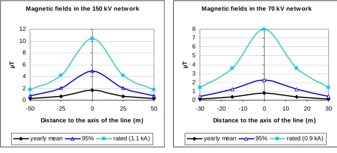
Assessment of the Electric and Magnetic field levels in the vicinity of the HV overhead power lines in Belgium.
Texte intégral
Figure
Documents relatifs
Exopodite biarti- culé plus court que l'endopodite avec article proximal plus large que le distal, celui-ci semi-ovalaire avec 7 tiges marginales lisses insérées du
To evaluate the influence of the resin on the insulation properties, it was also measured the thermal conductivity of a reference panel, realized with only Opuntia
L’archive ouverte pluridisciplinaire HAL, est destinée au dépôt et à la diffusion de documents scientifiques de niveau recherche, publiés ou non, émanant des
If the magnetic mode amplitudes are reduced, being for instance reduced to the fourth of the case just con- sidered in Figure 4, this differential heating is strongly attenuated as
In the absence of resonances, that will be specified below, the dramatic improvement on magnetic confinement induced by a low magnetic shear condition will be recalled in Section II
Die Resultate der Studie zeigen, dass trotz einem erhöhten Risiko zu psychischen Folgen eines Einsatzes Rettungshelfer Zufriedenheit und Sinn in ihrer Arbeit finden können und
Quanti fication of epidermal DR5:GFP reflux signals (Figure 2F; see Supplemental Figure 1 online) con firmed slightly reduced basipetal re flux for twd1 (Bailly et al., 2008)
L’archive ouverte pluridisciplinaire HAL, est destinée au dépôt et à la diffusion de documents scientifiques de niveau recherche, publiés ou non, émanant des
