HAL Id: hal-01816576
https://hal-mines-paristech.archives-ouvertes.fr/hal-01816576
Submitted on 15 Jun 2018
HAL is a multi-disciplinary open access
archive for the deposit and dissemination of
sci-entific research documents, whether they are
pub-lished or not. The documents may come from
teaching and research institutions in France or
abroad, or from public or private research centers.
L’archive ouverte pluridisciplinaire HAL, est
destinée au dépôt et à la diffusion de documents
scientifiques de niveau recherche, publiés ou non,
émanant des établissements d’enseignement et de
recherche français ou étrangers, des laboratoires
publics ou privés.
Optimal Offer of Automatic Frequency Restoration
Reserve from a Combined PV/Wind Virtual Power
Plant
Simon Camal, Andrea Michiorri, Georges Kariniotakis
To cite this version:
Simon Camal, Andrea Michiorri, Georges Kariniotakis.
Optimal Offer of Automatic Frequency
Restoration Reserve from a Combined PV/Wind Virtual Power Plant. IEEE Transactions on Power
Systems, Institute of Electrical and Electronics Engineers, 2018, 33 (6), pp.6155 - 6170.
�10.1109/TP-WRS.2018.2847239�. �hal-01816576�
Abstract— This paper presents a methodology for estimating
the optimal amount of automatic Frequency Restoration Reserve provided by an aggregation of renewable power plants. The increasing penetration of distributed weather-dependent renewable generation presents a challenge to grid operators. Wind and photovoltaic power plants are technically able to provide ancillary services, but their stochastic behavior currently hinders their integration into reserve mechanisms. In the methodology developed a Quantile Regression Forest model is used to forecast the aggregated production and a copula-based approach integrates the dependence between prices and renewable production. We then propose and compare three strategies to derive an optimal quantile of the combined production forecasts that can be used as basis to provide a reliable ancillary service to the System Operator. The methodology is evaluated using historical prices for energy and automatic Frequency Restoration Reserve along with production measurements from several renewable power plants.
Index Terms— Aggregation, Ancillary services, Flexibility,
Forecasting, Photovoltaic power systems, Smart grids, Virtual power plant, Wind energy
NOMENCLATURE
Indices
, Upward reserve , Downward reserve emp Empirical copula
k Forecast horizon
kurto Kurtosis of weather variable over grid points around plant
k
Product length of aFRR capacity
skew Skewness of weather variable over grid points around plant t Forecast runtime
Index of tree in Quantile Regression Forests
This paper was submitted for review on 12.04.2018. The research was carried as part of the European project REstable (Reference Number 77872), supported by the ERA-NET Smart Grids Plus program with financial contribution from the European Commission, ADEME, Jülich Research Center, Fundaçaõ para a Ciência e a Tecnologia.
S. Camal, A. Michiorri and G. Kariniotakis are with MINES ParisTech, PSL Research University, PERSEE - Center for Processes, Renewable Energies and Energy Systems, Sophia-Antipolis, 06904 France (email: simon.camal, andrea.michiorri, georges.kariniotakis each @mines-paristech.fr).
W , PV Wind and Photovoltaic plants
Sets
Xˆ Numerical Weather Predictions
S Portfolio of plants in the Virtual Power Plant Decision variables
R
Nominal value of the quantile selected for reserve
R
opt Nominal value of the optimal quantile for reserve k
, t
Eˆ Day-ahead energy offer [MW] k
, t
Rˆ Day-ahead symmetrical reserve offer [MW] Parameters
R
aˆ Expected activation probability for aFRR h
ˆ
Estimated mean in imbalance price regimes, for hour h *
i i,
Lagrange multipliers of Support Vector Regression (SVR)
b Affine coefficient of functional in SVR V
Coefficient of exogenous variable in day-ahead price model
cˆ, Cˆ Copula density, Copula cumulative distribution function
RE
ˆ
Expected day-ahead price spread between energy and reserve [€/MW.h]
RE
P
Random variable: day-ahead price spread between day-ahead energy and reserve [€/MW.h]
* RE ˆ
Expected real-time price spread between net penalties for energy and reserve [€/MW.h] *
RE P
Random variable: real-time price spread between net penalties for energy and reserve [€/MW.h]
t
White noise on day-ahead price moving average, at time t 1
X Y
Fˆ Inverse cumulated density function of aggregated production
forecast [MW] i
Auto-regression coefficient of day-ahead price at lag i m
Steepest gradient at iteration m of Gradient Boosting Tree K Kernel of Kernel Density Estimator Copula
Lˆ, Mˆ Load and Margin forecast at market level h
p
ˆ Estimated unconditional probability of imbalance energy price
regime, for hour h *
E
ˆ
Expected net energy imbalance price [€/MWh] E
ˆ
Expected energy price on day-ahead market [€/MWh] b
Im E
ˆ
Expected energy imbalance price [€/MWh] R
E
ˆ
Expected price for energy activated aFRR reserve [€/MWh]
R
ˆ
Expected capacity price on day-ahead aFRR market [€/MW.h]
Optimal Offer of Automatic Frequency
Restoration Reserve from a Combined PV/Wind
Virtual Power Plant
Simon Camal, Student Member IEEE, Andrea Michiorri,
George Kariniotakis, Senior Member, IEEE
R
ˆ Expected average symmetrical aFRR price including capacity and
activation [€/MW.h] *
R
ˆ
Expected net aFRR reserve penalty price for reserve deficit [€/MW.h] R
E R
ˆ
Expected average aFRR price (capacity+ activation energy) [€/MWh]
PRE,m
q Estimated quantile of price spread at iteration m i
R Infra-marginal reserve capacity at index i in the merit-order list
[MW]
aFRR demand activated by the TSO at each time-step [MW] ˆ
s
h2 Estimated log-normal variance of imbalance energy drop/spikeprice regime, for hour h
Moving-average coefficient of day-ahead price regression residual at lag j
Regression tree of loss gradient at iteration m of Gradient Boosting Tree
Regression tree of quantile response variable at iteration m of Gradient Boosting Tree
TS Thresholds in distribution of spike/drop imbalance energy prices
U Cumulated distribution function of production
V Cumulated distribution function of price spread Weight function of regression tree for learning set index i
Wˆ Wind power forecast at market level
Number of trees in the Quantile Regression Forests model X Multivariate explanatory variable for production forecast
RE P
X Multivariate explanatory variable for price spread forecast Installed aggregated active power capacity [MW] Random variable: aggregated power production [MW] Indicator function
I. INTRODUCTION
UE to their inherent dependency on weather conditions, the intermittent production of wind and photovoltaic (PV) power plants impacts the way power systems are operated, with consequences on the system stability and quality of service. However, studies have identified that wind and photovoltaic (PV) power plants show technical capabilities to provide Ancillary Services (AS) such as frequency support to the grid [1]. Moreover, Transmission System Operators (TSO), like that of Ireland, are starting to integrate specific regulations for frequency control from wind power plants into their grid codes [2]. Studies of the French TSO show that participation of wind power in downward reserve and balancing could generate a global economic revenue of 3 k€/MW.year [3].
Automatic Frequency Restoration Reserve (aFRR) is the second level of frequency control, deployed after Frequency Containment Reserve to restore frequency to its nominal value. Experiments conducted within the project Kombikraftwerk 2 in Germany have shown that aggregated renewable plants controlled by a Virtual Power Plant (VPP) can regulate their output according to aFRR signals, but with transient excursions outside the tolerance bands defined by TSOs‟ prequalification schemes [4]. Market conditions for aFRR are still heterogeneous in Europe, but regulators are moving towards advanced levels of harmonization to reach more liquid markets of balancing and reserve. The draft
regulation on electricity balancing published by the European Commission [5] requires TSOs to develop market methodologies based on pay-as-cleared pricing. Current discussions within ENTSO-E propose a minimal aFRR bid size of 1 MW, and that only integer values should be accepted [6]. The German regulator is considering shortening the lead-time of its aFRR tender from one week to one day, with a product length shortened to blocks of 4 hours [7]. Such a product length is coherent with the duration of consumption peaks and valleys. It is also likely to increase the opportunity for wind and PV to offer substantial reserve capacities.
Several studies have looked into AS offer strategies from renewables, including technical and economic constraints. A Belgian experiment [8] issued day-ahead offers of downward aFRR capacities for product lengths of 15 minutes. Forecasted production below a capacity dead-band (10-20% of installed capacity) was discarded for potential offers, because the quality of pitch-based power regulation was found to deteriorate in these low wind speed conditions. In case of sufficient forecasted production, volumes of 5 to 10 MW were proposed for the existing reserve market without affecting the market clearings. The observed reliability of the offer (defined as the difference in volume between offered reserve capacity and measured feed-in, compensated for any reserve activation) is 99.3%. In [9] Jansen models reserve bids based on opportunity costs or profit maximization. Capacity volumes are chosen from a forecast quantile, whose nominal value matches the observed reliability of reserve offers by conventional plants (99%-99.994%). The profit maximization bids use perfect price forecasting to place reserve offers at the marginal capacity price of the merit-order list, hence delivering an upper bound of revenues for a given offered volume. An analytical model of optimal quantiles for a joint day-ahead offer of primary reserve and energy is proposed by [10] for a wind power plant in Denmark: the expected revenue is found to increase from 3% to 12% depending on the methodology chosen. While the combination of renewables and storage for aFRR provision has been investigated, see for instance wind/pumped hydro in [11], aFRR offers originating from an aggregation of wind and PV have not been treated frequently in the literature. The interest of combining wind and solar power plant within the same VPP comes primarily from the industry itself since aggregators often develop portfolios integrating both technologies. This is the case developed within the frame of the EU demonstration project REstable, where a VPP of an aggregated capacity in the order of 100 MW is developed to provide aFRR [12]. The combination of Wind and PV to supply AS is valid in various climate zones, and may be a leading option for regions where hydro, which is a conventional renewable-based provider of AS, has limited resources. The interest of a VPP based solely on wind power and PV is also to propose a solution with reduced upfront investment costs compared to thermal plants, hydro plants and electrochemical storage: the marginal costs of wind power and PV are close to zero, and the required investment in control and software to meet with technical
demand R j m , g t m , q t i w max y Y . 1
D
qualification standards is comprised between 5% and 13% of the total investment for a wind farm [1]. The aFRR offer of a small VPP composed of wind power and PV, derived from the aggregated production forecast, was compared in [13] with aFRR offers issued separately by the wind and PV plants making up the VPP. In this case the aggregation permits to capture the dependence between production uncertainties of wind power and PV, and leads to higher reserve capacities than in the case of separate offers by each plant.
Precise production forecasts are a necessary input in reserve offering strategies. For the forecasting horizon of interest in the present paper (day-ahead, look-ahead time from 12h to 48h), the forecast of wind and PV production relies on Numerical Weather Predictions (NWP) [14]. An exhaustive review of the state of the art on existing methods is given in [15]. Among the existing models, in this work we consider the Quantile Regression Forests (QRF) model, which is a well-established probabilistic model for wind and PV power forecasting, and figures among the best performing models for both wind and PV forecasting [16]. Almeida et al. found that a training period shorter or equal to 15 days was sufficient for QRF prediction of PV power [17]. They also proposed to filter the training data by days showing an empirical distribution similar to the distribution of the NWP on the day to forecast, which improves performance. More advanced models applicable to both wind and PV are available but generally involve a higher computational burden or greater complexity, see for instance the approaches using gradient boosting proposed by Huang and Perry for PV [18] and Nagy et al for wind [19]. The forecast of aggregated solar or wind production is an emerging topic in the literature (see [20]– [22]). To our knowledge, little has been published on the aggregated forecasting of both wind and PV plants. The production forecast of a VPP combining wind and PV plants proposed in [13] is based on a model combining k-Nearest Neighbors and a bivariate Kernel Density Estimator. This model is adapted to aggregations where plants featuring the same technology experience similar weather conditions (i.e. located within the same region).
Having considered the state of the art of AS offer strategies and the forecasting of renewable energy production, this paper makes the following original contributions:
- A probabilistic forecast of the aggregated production of geographically dispersed PV and wind power plants, - A methodology to derive optimal day-ahead offers of
aFRR and energy using probabilistic forecasts of production and price spreads,
- A non-parametric copula that models the non-linear dependence between price spreads and VPP production, to adjust the reserve offer when renewable production is likely to affect prices,
- a comparison of the impact on revenue of using deterministic or probabilistic price forecasts.
To the best of the authors‟ knowledge, these topics have only marginally been treated together. The proposed integrated approach deals with the challenges of each part of
the complex modelling chain.
We begin by formulating the problem of optimal offers of aFRR and energy in Section II. The proposed methodology is presented in Section III and the methodology for production forecasting is detailed in Section IV. Strategies to derive offers are developed in Section V, simulated in Section VI and tested on a real-world case study in Section VII. We conclude in Section VIII.
II. PROBLEM STATEMENT
The objective of this work is to derive an optimal day-ahead offer of aFRR at 30-min resolution, provided by a VPP aggregating photovoltaic and wind power plants located in the same Control Area. The problem poses two main challenges:
1. We need to estimate a precise probabilistic forecast for the aggregated production of the VPP.
2. From this forecast, we need to derive reliable volumes of reserve that can be proposed on the existing ancillary services markets. To do this, we need to forecast day-ahead prices for energy and aFRR, but also aFRR activation probabilities and imbalance prices for energy. The interdependence between these prices and the renewable production could give useful information on when it is favorable for the VPP to offer aFRR. Considering that deterministic forecasting of imbalance energy prices and aFRR activation can be of limited value given the associated uncertainties, a probabilistic forecasting of the price spreads could lead to more robust decisions with respect to these uncertainties.
The modeling of a third logical step, i.e. the step involving disaggregation of the activated flexibility to individual power plants in the VPP, is not addressed in detail in this paper. For reference on this topic, see for instance the leader-following control strategy proposed by [23] for the coordination of aggregators offering AS. Finally, it is assumed that variations in technical characteristics among PV plants or wind plants (e.g. turbine technology for wind, panel/inverter technology or panel inclination for PV) do not significantly influence production forecasts and aFRR capacity offers.
III. OVERVIEW OF PROPOSED METHODOLOGY
A new methodology is proposed here to solve the aforementioned problem. The workflow is summarized in Fig. 1. It relies firstly on the probabilistic forecasting of the VPP aggregated production, based on Numerical Weather Predictions (NWP) and historical production records. The forecasting model is presented and discussed in Section 0. In the next step, an offer of symmetrical aFRR for the VPP is issued following the methodology proposed in Section V and taking the aggregated production forecast as input. Three alternative strategies to derive aFRR offers are proposed and compared.
1. Reliability-maximizing offers: these offers aim at respecting a high level of reliability in the provision of aFRR. They rely on a very low quantile of the aggregated
production forecast. The nominal value of this quantile is set to a constant that is close to the acceptable failure rates defined by TSOs when sizing AS (typically 0.006%-1% [9]).
2. Revenue-maximizing offers, independent from production: these offers maximize the revenue of energy and reserve by deriving an optimal quantile for reserve. This derivation is presented in Subsection V.A. It uses deterministic forecasts of reserve and energy prices which are presented in Subsection V.A.2. The introduction of a specific variable, the aFRR activation probability, is discussed in Subsection V.A.1. We describe this approach as “independent from production” to underline that the obtained quantile values do not depend on the production of the VPP. We compare these quantiles with quantiles based on a deterministic persistent price forecast and on perfect knowledge of price. The persistent price is expected to have a similar climatology to the perfect price, but with lower discrimination hence lower revenue from aFRR than for perfect knowledge of price.
3. Revenue-maximizing offers, dependent from production: Deterministic price forecasts and their errors are used as inputs in a probabilistic forecasting model of price spreads between energy and reserve. The dependence between these spreads and the production is modeled by non-parametric copulas described in Subsection V.B. Finally, the optimal quantile for reserve is obtained from the expected price spreads conditional on the VPP production.
In the last step, revenues and penalties for deployed energy and aFRR are simulated on a test period as described in Section VI. Realizations of the VPP operation (production forecast, measured production) over the test period are sampled. We simulate the net revenue for all operation samples available at a given time unit, similar to the Monte Carlo simulation proposed by [24].
Fig. 1. Methodology flowchart
IV. PROBABILISTIC FORECASTING OF AGGREGATED
PRODUCTION
Given that probabilistic forecasts are required for VPP production, making individual forecasts for wind and PV production, which is standard practice in applications, is no more convenient since these cannot be easily added. As a function of weather conditions or time of day, the percentages of wind and PV production may vary from null to nominal capacity within the mix. Given that different explanatory variables are needed to forecast each process, a highly adaptive forecasting approach is required to deal with the aggregation of both.
The NWP forecasts XˆWw and XˆPVp for each wind power plantwof the wind portfolioSWand each plant p of the PV portfolio SPV respectively are merged in (1) into a multivariate explanatory variable X used for the regression of t
the aggregated production:
p SPV
p t , PV W S w w t , W t Xˆ ,Xˆ X (1)The explanatory variable Xˆ(l)associated with a given plant of index
l
in (2) comprises: weather forecasts at the site of each plant at a horizon k, the same weather forecasts at horizon k-1 hour and k+1 hour, and statistical moments (standard deviation, skewness, kurtosis) of the distribution of weather variables over the grid points neighboring each plant. These statistical moments are considered as input to test whether higher diversity in NWP improves the aggregated production forecast.
l
kurto , k l skew , k l sd , k l k l k l k l Xˆ ,Xˆ ,Xˆ ,Xˆ ,Xˆ ,Xˆ Xˆ 1 1 (2)Recent measurements of power production are not considered as explanatory input here since previous studies [15] have shown that they contribute for horizons up to 6 hours ahead and do not improve the forecast model on the day-ahead horizon that is of interest in this paper. The aggregated wind and PV production is forecasted using a QRF model. This model evaluates in (3) a conditional distribution of the power production 1
kXt
t Y
Fˆ weighted by the explanatory variables, which are randomly selected by a parameter in each tree of index and tested within aggregated decision trees [24]. Each split at a node of the tree is carried out to maximize the diversity of variance within the subspace Sl of
the learning set defined by a leaf l. The number of trees grown must be sufficiently large to fit several times each training point i identified by the indicator function 1Yiy. The regression performance is usually quite insensitive to the number of variables randomly selected at each split, if it is higher than the recommended value for regression (1/3 of the number of explanatory variables) [24].
(3) QRF has been chosen for its ability to perform regression on multivariate inputs of large dimensions [24] and for its proven performance for individual wind [25] and PV [17] day ahead forecasting. Finally, the decorrelation of the explanatory variables obtained in the QRF by bagging and random variable selection is an interesting feature for differentiating various plants of the same typology. To validate the use of the QRF model, we benchmark it against a quantile linear regression model (QLR), fitted only on weather variables to avoid singularities in the covariance matrix due to high correlations between weather variables and their lagged counterparts or statistical moments. We also compare QRF with a gradient boosting tree (GBT) to serve as a non-linear benchmark. The GBT builds shallow decision trees improved iteratively by boosting. It is trained on a quantile loss function for each quantile of the distribution.
V. STRATEGIES FOR DAY-AHEAD OPTIMAL OFFER OF
ENERGY AND AFRR
Every day, a decision has to be made for the day ahead regarding the share of aggregated forecast production that will be dedicated to reserve. The remainder will be traded on the energy market. The target share dedicated to reserve is considered here as a quantile of the probabilistic production forecast given by (3), at nominal value R. In the case of reliability-maximizing offers, the nominal valueRequals a minimal risk of failure to provide the forecasted capacity. In both cases of revenue-maximizing offers, this nominal value is determined as a function of price forecasts (see Subsection V.A). The reserve capacity offerRˆt,k is then chosen in (4) as the minimum value of the aggregated production quantile
forecast
R t X k t Y Fˆ 1 at runtime t, over an horizon interval k.
This interval could be the entire day or a subset of shorter length.
R t X k t Y k k k , t min Fˆ Rˆ 1 (4)The energy offer Eˆtk at horizon k is given in (5) considering that the balancing market is operated following a single-price paradigm. In this case the theoretical optimal bid consists in offering the installed capacity if the forecasted day-ahead price is higher than the price for imbalance, and zero otherwise to maximize the arbitrage opportunity between the day-ahead market and the balancing market [26]. Considering the high uncertainties regarding the imbalance price for the day ahead, we choose here a more conservative bid which hedges the offer against imbalance penalties: the VPP will bid the mean of its production forecast, limited by the installed capacity ymaxand the reserve offer, which has priority over energy. This approach is in line with the risk-constrained energy offer proposed by [26] in a single-price balancing market, which is also set with reference to the mean of the forecasted production.
k t
Eˆ = min
ymaxRˆt,k, 𝔼
Ytk
(5)A. Production-independent Optimal Quantile for aFRR
We consider now that the aim of the VPP is to formulate revenue-maximizing offers on day-ahead markets for both energy and aFRR. It is assumed that the decisions of the VPP have no temporal dependence over a sequence of time steps. This assumption is justified here by the lack of decisions impacting the available production, such as trading in the intraday market or use of storage, between the day-ahead offer and the deployment of energy and reserve. This simplifies the
problem of maximizing the summed daily revenue as maximizing the expected revenue over each time unit [27].
This type of problem can be solved analytically and boils down to the derivation of an optimal quantile [10], following the theory of terminal linear losses [28]. We show in Section A.1 of the Annex how to obtain the optimal quantile for aFRR, looking for an optimum of the expected opportunity loss, and using Leibniz‟s rule to compute the derivative with respect to the amount of reserve offered. We assume at this stage that the prices involved in the energy and reserve market are estimated by a deterministic forecast. The derivation assumes the following market conditions:
- The VPP acts as a price taker in the day-ahead market, and is awarded the marginal price in the reserve auction; - The decisions taken by the VPP are risk-neutral;
- The energy opportunity cost for upward activated reserve is remunerated by the TSOs;
- The VPP pays the TSOs for the energy not produced during activation of downward reserve.
The optimal quantile is given in (6) for symmetrical aFRR, based on expected prices for energy and reserve. The
N i y i Y l , x l S k t Y . , x S : j Card x , y Fˆ 1 1 1 1 1 j t, i t, X t X X R opt
forecast of these expected prices (noted below with
ˆ
is explained in the next subsection.* E * R E R E R R E R R R E R E R R E R R R R opt ˆ ˆ ˆ ˆ. a ˆ ˆ. a ˆ ˆ ˆ ˆ ˆ. a ˆ ˆ. a ˆ ˆ ˆ (6) * RE RE RE * E * R E R E R ˆ ˆ ˆ ˆ ˆ ˆ ˆ ˆ ˆ
In the equation above R stands for reserve, E for energy,
R
E for energy associated with reserve activation.aˆRis the expected probability of the VPP being activated among bidders present in the merit-order list, for upward and downward aFRR. In summary, the optimal quantile represents the balance between the lost gain opportunity (proportional to the revenue price spreadˆRE) and the increase in penalty losses (proportional to the penalty price spreadˆ*RE) when
reserve is more expensive than energy. As demonstrated in (6), estimating the optimal quantile involves forecasting two types of quantity, i.e. the probability that the VPP will be activated and market conditions. The proposed methodology to derive and forecast these quantities is presented in the following two subsections.
1) Estimation of aFRR Activation Probability
Equation (6) implies forecasting the probability that the VPP will be activated for aFRR. Here, we present how this probability is estimated based on historical data from aFRR auction settlements and activations, while in the next sub-section we present how it is forecasted. We assume that the position of the VPP on the merit-order list (MOL) has a uniform probability. Although the low marginal costs of the renewable plants within the VPP would probably induce a low marginal price from the VPP, it is hazardous to assume that the VPP will be systematically selected among the cheapest offers, at least in aFRR markets that are penetrated by hydro or that integrate large amounts of wind and PV. Therefore, the VPP is considered as equally likely to be located anywhere in the merit-order. The activation probability is then estimated based on (7) and is valid for both upward and downward activation. At each activation time step, the activation probability equals the sum of infra-marginal reserve capacities that are situated below the reserve activated by the TSO in the merit-order list (for these capacities, the indicator function returns 1, 0 otherwise), divided by the sum of the allocated reserve as a result of the aFRR auction.
MOL j j MOL i demand R i R i R R . R a 1 (7)The model proposed here is based on the available history of reserve activations for all reserve suppliers. However, we can tune the model to the historical activation records of the VPP itself, if such data are available, in order to predict the VPP‟s actual probability of activation. This is expected to be the case in the future, when intermittent renewable VPPs enter
the aFRR market. An alternative model for activation probability proposed by [29] is based on the density of the wind forecast error. This was devised for sizing reserve and does not include tendered reserve volumes. It is therefore less adapted to the forecast of aFRR market conditions than our model in (7).
The activation probability obtained from this approach regarding the tendered and activated capacities on the aFRR market in Germany shows a high variability and discrepancies between upward and downward activation. In Fig. 2 this activation probability is averaged on a rolling daily mean to show tendencies more clearly. The probability of a reserve being activated has an impact on the potential revenue of the VPP. A downward reserve paid for capacity (after being selected in the tender) that is rarely activated (no need to curtail the production and day-ahead energy offer, no payment to TSO for downward energy activation), is the best-case for the VPP profitability. Conversely, an upward reserve paid for capacity that is rarely activated is likely to constitute the worst-case for profitability, as production is curtailed and the day-ahead energy offer has to be reduced.
Forecast errors on load and renewable production are correlated to the probability of reserve activation: in a scenario of high penetration of renewable energy, an evaluation of the activation probability should consider renewable production forecast errors as an important factor. The diagram on the left of Fig. 3 shows that the aFRR activation probabilities (January 2015-December 2016, 30-min resolution) are correlated with load forecast errors. Large negative load forecast errors, where grid operators require less reserve power than forecasted to ensure balance, are usually associated with significant reserve activation probability comprised between 0% and 40%. We observe that large positive load forecast errors, where load has been largely underestimated, are relatively rare. As expected in this case, only upward reserve is activated to supply more power to the grid. Low activation probabilities for large deviations could indicate that balance was mainly attained via services other than aFRR.
Fig. 2. Activation probability computed on German data. Downward aFRR in red, upward aFRR in blue. January to March 2016
The relation with wind generation forecast errors (at the control area level) shown onthe right diagram of Fig. 3 is less pronounced, and the activation probabilities are distributed rather uniformly on the scale of wind forecast errors. Still, large negative wind forecast errors seem to trigger more upward reserve activation than positive errors do for downward activation. The downward activation probabilities are slightly lower than the upward probabilities, and the same goes for load forecast errors: this may indicate that the upward reserve is dimensioned with a higher margin than its downward counterpart for the specific dataset used. In a scenario of very high penetration of wind power in this electricity market, the forecast of wind power at market level could benefit from the aggregation effect and reduce its overall error range on average. Meanwhile, the frequency of large or extreme forecast errors could increase when forecasting models propagate systematic errors on the zone‟s wind farms. To conclude, it appears that regional or national wind forecasts and their errors can be valuable explanatory variables for forecasting aFRR activation probability.
Fig. 3: Observed aFRR activation probabilities and forecast errors on load and wind production for Germany (data 2015-2016).
2) Forecast of Market Conditions
As explained in the previous section, in order to derive an optimal quantile for aFRR through (6) we need a forecast of the price spreads between energy and reserve. This involves forecasting the following expected market conditions which compose the price spreads:
- day-ahead and imbalance energy prices, ˆE ˆImE b, - aFRR capacity price and average price (capacity +
activation energy) ˆR, R E R ˆ ,
- aFRR activation probability aR.
We decide to forecast each price separately instead of directly forecasting price spreads because each price exhibits specific market dynamics. A state-of-the art forecasting technique is implemented for each price, when available. As the scope of this paper is mainly focused on the technical capacity of the VPP to offer ancillary services, price forecasts are developed here only to test the methodology. The forecast models of the different market conditions are presented in Section B of the Annex.
B. Optimal Quantile Dependent on Renewable Production
In a context of very high penetration of renewables, it is likely that VPP production will show some correlation with energy and reserve prices. The idea is that the VPP production profile would present some similarity with the aggregated Wind+PV production at market level, as has been observed in the case of wind power plants [36]. To obtain the optimal quantile for reserve (see Section A.2 in the Annex), we evaluate as in (8) the expected price spreads conditional to the (forecast) VPP production, 𝔼
PRE Y
and 𝔼
PRE* Y
beingfor the day-ahead and the imbalance respectively:
𝔼
P Y yˆ fˆ Y yˆ d RE P RE (8)The problem is analytically tractable if the joint densities of prices and production are modeled with simple approaches such as bivariate normal distribution, which are of limited use in practice because renewable production and prices are not normally distributed [36]. A regression approach could be employed to derive these conditional expected price spreads, for instance using a bivariate kernel density estimation. We choose here a density-based regression using a non-parametric copula. Copulas have the advantage of decoupling the dependence model from the marginal distributions, which can be forecast with various approaches without any impact on the dependence model. Copulas also deliver a probabilistic description of the dependence between production and prices. They give for instance the most likely price spreads conditioned by renewable production forecast. If the VPP production is high, there will be probably a high share of renewable in the market, therefore-a high probability of low day-ahead energy price. Finally, this gives a high probability of favorable day-ahead spread for reserve. In (9) we use the Kernel Density Estimation (KDE) copula [37] to evaluate the conditional density of the price spread PRE with respect to
VPP production Y . The Epanechnikov Kernel is used for price spread and power production. An alternative not tested here could be to use the Beta Kernel for the production, which is well suited to bounded variables [37]. The two smoothing bandwidths and are chosen following the Scott rule:
fˆ
.
cˆ
F
yˆ
,
F
,
fˆ
Y yˆ PRE Y PRE RE P ℝ (9)The goodness of fit of dependence is quantified in (10) by a Cramér-Von Mises statistic CvM [38] comparing the distribution of the copulaCˆ
u,v with the distribution of the empirical copulaCˆemp
u,v .
, h F v K h y F u K h . h . N v , u cˆ v i RE P V u i Y N i U v u
1 1
0,1 ) , (u v
u
,
v
Cˆ
.
v
,
u
Cˆ
v
,
u
Cˆ
N
CvM
emp , empd
2 1 0 2
N i v i RE P F , u i y Y F emp N v , u Cˆ 1 1 1 (10)The distribution of price spread is obtained by a gradient boosting tree model trained on the feature vector ,t
RE P X
gathering in (11) the deterministic forecast of the prices composing the spread and the associated errors.
REt,
* t, RE t, RE t, RE * t, RE t, RE t, RE P ˆ ,ˆ ,ˆ ,ˆ X (11)The estimated quantile of level ,m
RE P
q is obtained in (12) after m iterations by the iteratively built regression tree
m , q
t based on the steepest gradient mof the quantile loss function L.
x Fˆ y x q t, RE P RE P m , RE P inf y: X
x t
x t
x qPRE,m q,m m q,m1
N i i, m i m , g i m , RE P i, RE m L P q x t. x ,g 1 1 argmin (12)Note that we do not model the tails separately as for instance in [39], because we consider a risk-neutral VPP and therefore accept forecast errors on the rare extreme price spreads.
VI. EVALUATION OF VPPNET REVENUE FROM ENERGY AND AFRR
The optimal offer of energy and aFRR generates revenue for the VPP on the day-ahead markets of energy and aFRR. This revenue is computed using observed prices for energy and aFRR capacity. The penalties and revenues occurring in real-time are computed using observed aFRR activation probabilities and prices for upward and downward reserve, and observed imbalance energy prices. If the VPP production in real-time is lower than the summed offer of aFRR capacity and energy, the amount of energy delivered is reduced and energy penalties are paid to avoid failure on reserve deployment. The VPP net revenue sums up revenues and penalties from the day-ahead stage and the real-time stage.
The obtained revenue at a given time unit is computed for a single combination of prices and VPP operation. The VPP operation is defined by the forecasted and measured production. To increase the robustness of our revenue evaluation, we sample realizations of the VPP operation and compute revenues at each time unit on a set of operation samples, with the prices observed at that time unit.
VII. CASE STUDY
A. Description of the Case Study
The methodology is evaluated on a real-world case study of a VPP, which jointly offers energy and symmetrical aFRR on a day-ahead auction with an aFRR product length of 4 hours. Real production data covering the period September to December 2015 are used to tune the forecasting models, while data from January to March 2016 are employed to evaluate them..
The VPP‟s offers have to be placed before gate closure time at 9h00 UTC, each day and are evaluated over the 3 month testing period (January-March). The VPP combines wind and PV plants operating in France, with a total capacity of 42.3 MW and a 24% share of PV. The distance between any two power plants varies between 30 km and 700 km. These relative high distances imply that spatiotemporal correlations in the production are rather low. This is an interesting feature for the present application, i.e. the more diverse the production profiles are within the VPP, the less variable its power output will be, and likely with higher minima.
B. Aggregated Production Forecast
Probabilistic forecasts are generated using historic production data and NWPs from the European weather forecasting center ECMWF. The NWPs used are the predictions published at 00h00, in order to consider delivery delay and have sufficient time to process the forecast before gate closure. The training period covers 5 months (September-December). A QRF model is trained on the NWPs and the historical production data. The explicative value of NWP variables is evaluated by the model via an “importance” factor, which quantifies the increase in regression error when values of the selected variable are randomly permuted and tested against out-of-bag samples [40]. The variables with higher importance are listed in Table I. We note that weather variables have similar importance levels among plants of the same technology. The spatial distribution coefficients were found to improve the aggregated forecast for PV plants only.
1) Reliability
The forecast model is evaluated over the testing period stipulated above. The rank histogram of the probability integral transform (PIT) of the forecast shows in Fig. 4 an over-dispersive behavior on low quantiles and under-dispersive behavior on 20%-50% quantiles. The reliability is marked by the sampling effect created by the short duration of the validation period and by the errors of the QRF model.
2) Quantile Score
We select the Quantile Score (QS) as a forecasting skill score given that it is a probabilistic score widely used by the forecasting community [16]. The monthly-averaged QS of the QRF forecast is comprised between 0.023 and 0.026 over the test period, with an improvement of -55% and -30% against the QLR model and GBT model respectively (Table II). The GBT model has been trained with 2000 trees of depth 3 and
shrinkage of 0.01, the optimal number of trees for each quantile is obtained by 5-fold cross-validation. The performance of QRF is worse than the best forecasts on single wind or PV plants (maximum monthly-average QS of 0.022 for [18] and [19]) but in line with satisfactory wind power forecasts (monthly-average QS of 0.030-0.045 for [41], [42]). For this VPP dominated by wind power, the highest forecast errors of the QRF model in terms of Continuous Ranked Probability Score (CRPS) seem to take place at periods with significant solar radiation, which are located in the middle zone of the forecast horizon (Fig. 5). The gradient boosting model interestingly performs similarly to QRF when PV and wind produce both at daytime, but is worse at night when wind is the only source of power. Considering the context close to operational conditions, we find that the forecasting performance is sufficient for the present application.
TABLE I
FEATURES WITH MOST IMPORTANCE FOR QRFFORECAST
Variables PV Wind NWP SSRD, Temp U100,V100,W100 Lagged NWP SSRD.k-1/k+1 Temp.k-1 U100.k-1, V100/W100.k-1/.k+1 Spatial distribution NWP Temp.sd, Temp.skewness - Legend:
- SSRD: solar surface radiation downwards
- U100/V100/W100: zonal/meridional/absolute wind speed at 100 m - Temp: air temperature at 2 m
- k-1: previous hour
Fig. 4. PIT rank histogram of aggregated forecast
TABLEII
MONTHLY-AVERAGE QUANTILE SCORE [P.U.], AGGREGATED FORECAST
Model January February March
QRF 0.023 0.026 0.024
GBT 0.031 0.033 0.032
QLR 0.049 0.057 0.054
Fig. 5. Continuous Ranking Probability Score (CRPS) as a function of the forecast horizon for the QRF and the benchmarks QLR and GBT
C. Day-ahead Joint Offer of aFRR and Energy
The VPP simultaneously offers energy and symmetrical aFRR before noon of the previous day, using the QRF aggregated production forecast, and price forecasts in the case of a revenue-maximization strategy. The probabilistic forecast of the VPP production and the associated aFRR offers are illustrated in Fig. 6.
1) Deterministic Price Forecasts
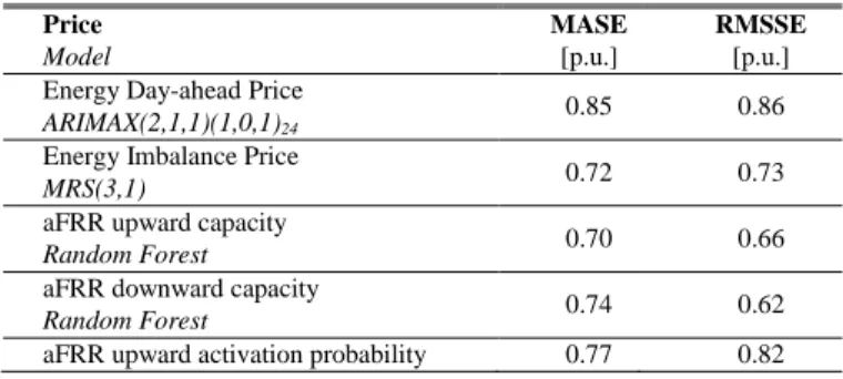
We forecast energy and reserve prices at 00h00 the day before (horizon of 24h to 48h). All price forecasts are based on a sliding window of 150 days for training data. The forecasts are evaluated on a testing dataset of German prices [33]spanning from January to March 2016. The reserve penalty is assumed here to be 5 times the reserve capacity price, as currently set by the French TSO [43]. We use error metrics that scale the forecast error by the error of daily persistence, i.e. the Mean Absolute Standard Error (MASE), and the Root Mean Square Scaled Error (RMSSE) [32]. If the scaled error is lower than 1, the forecast shows improvement against persistence. Price forecast errors are reported in Table III. The error levels for the energy price are coherent with similar studies based on auto-regressive or ARIMA models ([31], [30]). The forecast of aFRR capacities shows lower errors because daily persistence is strongly penalized on the first days of the week, which reproduce the valley-hour prices of the weekend. The error on imbalance price is lower than persistence mainly because the forecast has less bias than persistence. There is still significant room for improvement in capturing the variance correctly.
TABLEIII
FORECAST ERRORS FOR ENERGY AND aFRR PRICES
Price Model MASE [p.u.] RMSSE [p.u.] Energy Day-ahead Price
ARIMAX(2,1,1)(1,0,1)24
0.85 0.86
Energy Imbalance Price
MRS(3,1) 0.72 0.73
aFRR upward capacity
Random Forest 0.70 0.66
aFRR downward capacity
Random Forest 0.74 0.62
PCA+SVR
aFRR downward activation probability
PCA+SVR 0.74 0.77
aFRR upward average price
SVR 0.84 0.87
aFRR downward average price
SVR 0.84 0.82
2) Probabilistic Forecast of Price Spreads
A training period of 60 days was found sufficient for the gradient boosting model, using 5000 trees and a shrinkage
parameter of 0.01. The forecast of the spread for revenue prices is reliable on low quantiles (deviation of nominal rate below 3%), and underestimates higher quantiles (not surprising considering that the deterministic forecasts do not capture spikes). The quantile scores improve between 20% and 45% compared to climatology for quantiles lower or equal to 70%. Above this nominal value, the improvement is scarce which is in line with the findings for reliability.
Fig. 6. Aggregated production probabilistic forecast with QRF, confidence intervals in shades of blue/purple. Measured production in black. Risk-minimization aFRR offer in gray. Revenue-maximization aFRR offers in red based on the copula dependence, in blue based on deterministic price forecast, in
green based on persistence price forecast.
Fig. 7 shows that spreads observed over a 60-days period (February-March) fall on average within the central part of the forecast distribution, with a slightly positive spread. If we look at maximum spreads for a given hour of day (red curve), we observe spikes located outside the average forecast envelope during the two consumption peaks at mid-day and early evening. These are due to rare activation peaks where plants with a higher marginal price enter the merit-order. The minimum observed spreads for each hour of day (green curve) have lower levels during the daytime, and remain within the forecast envelope: the forecast model correctly captures low day-ahead prices.
Fig. 7: Day-ahead probabilistic forecast of revenue price spread between reserve and energy, obtained by a gradient boosting tree model. Prediction
intervals between 20% and 90%. Forecasts averaged at same hour of day.
3) Dependence between Price Spreads and Production
The KDE copulas are built on the VPP production and price spreads observed during the training period. The resulting copula density in the upper plot of Fig. 8 indicates that high VPP production is frequently associated with high price spreads on revenue, whereas low production levels are mostly linked with average spreads. This nonparametric copula detects asymmetrical tail dependences (high density for high quantiles, low density for low quantiles) and dissymmetrical densities for low price spreads and low production. The high price spreads on revenue occur when energy prices are low or the reserve activation price is high. High renewable production at very low marginal cost is known to produce low prices on energy markets, so the dependence structure detected by the copula in this zone is in line with practical experience. We also observe that medium levels of VPP production occur most frequently when revenue spreads are low, which usually occurs during the day.
To compare with the nonparametric copula, we fit parametric copulas by maximum likelihood estimation using the function “BiCopSelect” of the R package “VineCopula” [44]. A Joe-Frank copula (mostly symmetrical density and light upper-tail dependence) is selected for the dependence between day-ahead price spread PREand production Y, while
10 % 20 % 30 % 40 % 50 % 60 % 70 % 80 % 90 %
a Tawn 2 copula is selected for the dependence between imbalance price spread *
RE P
and production (asymmetrical density and asymmetrical tail dependences). The Cramér-von Mises statistic of the parametric copulas is higher than the KDE copulas (3.4 times higher for
PRE,Y
and 2.3 timeshigher for
PRE* ,Y
), and thus the KDE copula is closer to theobserved dependence structure in the learning data. Does this tighter fit lead to overfitting on the estimated quantile for aFRR? Although the parametric copulas partly detect the tail behaviors in the dependences, they tend to put more weight on the central part of the price distribution than the KDE copula, hence delivering higher quantiles for aFRR. The mean absolute error on the forecast of the optimal quantile for aFRR is 4.3% for the KDE copula, lower than the 5.0% for the parametric copulas.
The lower plot in Fig. 8 represents the copula density with a modified VPP portfolio where PV accounts for 75% of the installed capacity. In this case the dependence between high productions and high spreads is less pronounced; it is now higher with low spreads (typically when the sun shines during the daytime).
4) Optimal Quantile and Net Revenue
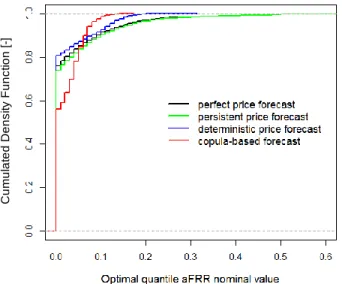
The cumulative density function (CDF) of optimal quantiles for aFRR obtained from the different price forecasts is presented in Fig. 9. The nominal value is most frequently zero, when the revenue price spread is negative (occurs e.g. at high energy prices, or for large activations of downward reserve). We see that the optimal quantiles are distributed on low values (0%-40%). The distribution of deterministic price forecast is close to the distribution of perfect price in the 0%-10% range of nominal values, but does not capture the high tail of optimal quantiles. The copula-based forecast issues less dispersed quantiles, influenced by the forecast of VPP production. Finally, we set at 1% the constant quantile value of the reliability-maximizing offer (ref. Section V), 1% being the maximum failure risk that a TSO is supposed to tolerate.
We evaluate the failure risk for each offer strategy by a Rate
of Under-Fulfillments (RUF) criterion [13], defined as the
frequency of timestamps for which the measured VPP production is inferior to the offered reserve capacity over the test period. The offer strategies have a RUF of between 0.1% and 2%, mostly due to the reliability of the probabilistic production forecast and the low values of quantiles dedicated to reserve. The RUF of the reliability-maximizing strategy is 1.3%. The highest RUF is 1.9% for the offer with persistence price forecast, and the lowest RUF is 0.1% for the strategy with the optimal quantile dependent on production, the latter having few under-fulfillments because its highest quantile values are lower than for the other strategies. This evaluation is limited by the available temporal resolution of production time series (here 30-min averaged). It also does not consider technical constraints that may impede a reliable regulation of power at low levels (wind turbines shutdowns were observed while down-regulating for a frequency response test in the Kombikraftwerk 2 project [4]).
We sample realizations of the VPP operation during the test period to evaluate the revenues of each strategy for diverse VPP operation conditions. The number of samples of VPP operations is 40 for each market time unit. Prices of the test period are characterized in Table IV. Results of the revenue calculation in Table V show an increase in net revenues when offering jointly aFRR and energy, reaching a maximum mean daily net revenue of 34.91 €/MW.h. The reliability-maximizing offer yields a similar net revenue to the revenue-maximizing offers based on deterministic forecasts (26.43 €/MW.h and 26.33 €/MW.h). The Conditional Value at Risk at 1% (CVar1%) is lower when offering both energy and reserve instead of energy only for all approaches. This indicates that adding aFRR increases the risk on net revenue, and advocates offering methods that are more risk conservative.
Fig. 8: Normalized density of copulas modelling dependence between price spread for revenue and VPP production:75% capacity from Wind, by KDE Copula (top left), 75% capacity from Wind, by Joe-Frank copula (1.39,0.95) (top right), 75% capacity from PV, by KDE Copula (bottom)
12
Fig. 9: CDF of aFRR optimal quantile
TABLE IV
CHARACTERISTIC PRICES DURING TEST PERIOD
Day-ahead energy price [€/MWh] Imbalance energy price [€/MWh] aFRR Upward average price [€/MW.h] aFRR Downward average price [€/MW.h] Average Price 23.7 20.7 41.5 0.9 Minimum Price -20.0 -630.6 33.8 -152.7 Maximum Price 53.5 634.5 239.9 11.3 TABLEV
RESULTS OF THE OFFER OF ENERGY AND aFRR
Mean daily net revenue for energy only is 25.05 €/MW.h Average reserve offered Mean daily net revenue Energy + aFRR Mean daily net revenue variation Energy + aFRR vs Energy CVar1% net revenue variation Energy + aFRR vs Energy Units MWp % of €/MW.h % €/MW.h Reliability-Maximizing Strategy 0.103 26.43 +5.5% -25 Revenue-Maximizing Strategy, production-independent 0.040 26.33 +5.1% -138 Revenue-Maximizing Strategy, production-dependent 0.038 26.40 +5.4% -8
Benchmarks for Revenue-Maximizing Strategy, production-independent Perfect price forecast 0.057 34.91 +36% -18 Persistent price forecast 0.055 27.50 +10% -12 TABLE VI SENSITIVITY ANALYSIS ON
PRODUCT LENGTH AND ENERGY PRICES (NO SAMPLING) APPROACH WITH DETERMINISTIC PRICE FORECAST
Mean daily net revenue variation Energy + aFRR
vs Energy
Unit %
Reference Energy Price- varying product length
4 hours +5.1%
1 day +3.9%
Product Length of 4 hours – varying energy price
Reference Energy price
- 10% +8.2%
Reference Energy price
- 20% +9.2%
Reference Energy price
- 30% +10.2%
Reference Energy price
- 40% +11.4%
Reference Energy price
- 50% +12.5%
5) Sensitivity Analysis
Energy markets are oriented towards lower prices due to the penetration of renewable energy at near-zero marginal costs and other factors. To test the sensitivity of the present method in a context of high penetration of renewables, we linearly reduce the energy prices (revenue price and penalty price), while keeping the reserve prices constant. We assume that reserve, being a product of high added value with limited availability, will see its price remain stable. We then compute offers based on deterministic price forecasts and the original (not sampled) VPP production and its forecast.
The optimal quantile for aFRR increases as energy prices decrease. Table VII shows that the additional mean net revenue increases linearly with decreasing energy prices. An aFRR product length of 1 day instead of 4 hours leads to a lower increase in net revenue.
VIII. CONCLUSIONS AND DISCUSSION
This paper proposes a novel methodology for the joint day-ahead offer of aFRR and energy by a VPP composed of wind and PV plants located in different climatic zones. It is based on an aggregated forecast of the VPP production based on a QRF model that is shown to have satisfactory performance over the testing period. The monthly-averaged QS ranges from 0.023 to 0.026.
The operator of the VPP can then opt either for a strategy offering aFRR with a minimal risk of underfulfilment, or strategies aiming at a higher combined revenue from aFRR and energy. Offers of aFRR in the revenue-maximizing strategies are derived by an optimal quantile using price forecasts. Prices are forecasted with deterministic models, the MASE is comprised between 0.70 and 0.85, which shows moderate improvement relative to persistence. Energy offers are adjusted as a function of aFRR offers and expected
0.0 0.1 0.2 0.3 0.4 0.5 0.6 0 .0 0 .2 0 .4 0 .6 0 .8 1 .0
Optimal quantile aFRR nominal value
C u m u la te d D e n s it y F u n c ti o n [ -]
perfect price forecast persistent price forecast deterministic price forecast copula-based forecast