HAL Id: hal-00725590
https://hal.archives-ouvertes.fr/hal-00725590
Submitted on 27 Aug 2012
HAL is a multi-disciplinary open access
archive for the deposit and dissemination of
sci-entific research documents, whether they are
pub-lished or not. The documents may come from
teaching and research institutions in France or
abroad, or from public or private research centers.
L’archive ouverte pluridisciplinaire HAL, est
destinée au dépôt et à la diffusion de documents
scientifiques de niveau recherche, publiés ou non,
émanant des établissements d’enseignement et de
recherche français ou étrangers, des laboratoires
publics ou privés.
3D Model Retrieval based on Adaptive Views Clustering
Tarik Filali Ansary, Mohamed Daoudi, Jean-Philippe Vandeborre
To cite this version:
Tarik Filali Ansary, Mohamed Daoudi, Jean-Philippe Vandeborre. 3D Model Retrieval based on
Adaptive Views Clustering. 3rd International Conference on Advances in Pattern Recognition (ICAPR
2005), Aug 2005, Bath, United Kingdom. �hal-00725590�
3D Model Retrieval based on
Adaptive Views Clustering
Tarik Filali Ansary1, Mohamed Daoudi2, Jean-Phillipe Vandeborre1
1 MIIRE Research Group
(GET / INT / LIFL UMR USTL/CNRS 8022) {filali, vandeborre}@enic.fr
2 Universit´e Fran¸cois-Rabelais
Laboratoire d’Informatique de Tours (EA 2101) [email protected] http://www-rech.enic.fr/miire
Abstract. In this paper, we propose a method for 3D model indexing based on 2D views, named AVC (Adaptive Views Clustering). The goal of this method is to provide an optimal selection of 2D views from a 3D model, and a probabilistic Bayesian method for 3D model retrieval from these views. The characteristic views selection algorithm is based on an adaptive clustering algorithm and using statistical model distribution scores to select the optimal number of views. Starting from the fact that all views do not contain the same amount of information, we also introduce a novel Bayesian approach to improve the retrieval. We finally present our results and compare our method to some state of the art 3D retrieval descriptors on the Princeton 3D Shape Benchmark database.
1
Introduction
The use of three-dimensional image and model databases throughout the Internet is growing both in number and size. The development of modeling tools, 3D scanners, 3D graphic accelerated hardware, Web3D and so on, is enabling access to three-dimensional materials of high quality. In recent years, many systems have been proposed for efficient information retrieval from digital collections of images and videos. However, the solutions proposed so far to support retrieval of such data are not always effective in application contexts where the information is intrinsically three-dimensional. A similarity metric has to be defined to compute a visual similarity between two 3D models, given their descriptions.
For example, Kazhdan et al. [1] describe a general approach based on spheri-cal harmonics. From the collection of spherispheri-cal functions spheri-calculated on the voxel grid of the 3D object, they compute a rotation invariant descriptor by decom-posing the function into its spherical harmonics and summing the harmonics within each frequency. Then, they compute the L2-norm for each component.
The result is a 2D histogram indexed by radius and frequency.
In 3D retrieval using 2D views, the main idea is that two 3D models are sim-ilar, if they look similar from all viewing angles. Funkhouser et al. [2] apply view
based similarity to implement a 2D sketch query interface. In the preprocessing stage, a descriptor of 3D model is obtained by 13 thumbnail images of boundary contour as seen from 13 view directions. Using aspect graphs, Cyr and Kimia [3] specify a query by a view of 3D objects. A descriptor of 3D model consists in a number of views of the 3D models. The number of views is kept small by clustering views and by representing each cluster with one view, which is repre-sented by a shock graph. Schiffenbauer [4] presents a complete survey of aspect graphs methods. Using shock matching, Macrine et al. [5] apply indexing using topological signatures vectors to implement view based similarity matching more efficiently. Recently, Chen et al. [6] defend the intuitive idea that two 3D models are similar if they also look similar from different angles. Therefore they use 100 orthogonal projections of an object and encode them by Zernike moments and Fourier descriptors. They also point out that they obtain better results than other well-known descriptors. Tangelder and Veltkamp [7] present a complete survey on 3D shape retrieval.
In this paper, we propose a method for 3D model indexing based on 2D views, named AVC (Adaptive Views Clustering). The goal of this method is to provide an optimal selection of 2D views from a 3D model, and a probabilistic Bayesian method for 3D models indexing from these views. This paper is organised in the following way. In section 2, we present the main principles of our method for characteristic views selection. In section 3, we present the Bayesian Information Criteria (BIC). In section 4, our probabilistic 3D models indexing is presented. Finally, the results obtained from a collection of 3D models are presented showing the performances of our method. We compare our method to some state of the art 3D retrieval descriptors on the Princeton 3D Shape Benchmark database.
2
Selection of characteristic views
Let Db= {M1, M2, . . . , MN} be a collection of N three-dimensional models. We
wish to represent each 3D model Mi by a set of 2D views that best represent
it. To achieve this goal, we first generate an initial set of views from the 3D model, then we reduce it to the only views that best characterise the 3D model. This idea comes from the fact that all the views of 3D model do not have equal importance: there are views that contain more information than others.
In this paragraph, we present our algorithm for characteristic views selection from a three-dimensional model.
2.1 Generating the initial set of views
To generate the initial set of views for a model Mi of the collection, we create
2D views (projections) from multiple viewpoints. These viewpoints are equally spaced on the unit sphere. In our current implementation, there are 320 views. The views are silhouettes only, which enhance the efficiency and the robustness of image metric. Orthogonal projection is applied in order to speed up the retrieval process and reduce the size of the used features. To represent each of these 2D
views, we use 49 coefficients of Zernike moment descriptor [8]. Consequently to the use of Zernike moments, the approach is robust against translation, rotation and scaling.
2.2 Characteristic views selection
As every 2D view is represented by 49 Zernike moment coefficients, choosing a set of characteristic views that best caraterise the 3D models (320 views), is equivalent to choose a subset of points that represent a set of 320 points in 49 dimensions space. The problem of choosing X characteristic views that best represent a set of N = 320 views, is well known as clustering problem.
Data clustering is a well known problem in the Mathematical and Computer-Science communities. The literature in this domain is huge. One of the widely used method is K-means [9]. Its attractiveness lies in its simplicity and in its local-minimum convergence properties. However, it has one main shortcomming: the number of clusters K has to be supplied by the user.
As we want from our method to adapt the number of characteristic views to the geometrical complexity of the 3D model, using K-means is not suited. To avoid this problem, we use a method derivative from K-means. Instead of a fixed number of clusters, we propose to use a range in which we will choose the best number of clusters. In our case the range will be [1, . . . , 40]. In this paper, we assume that the maximum number of characteristic views is 40. This number of views is a good compromise between speed, descriptor size and representation.
We proceed now to demonstrate how to select the characteristic views set and also how to select the best K within the given range. In essence, the algorithm starts with K equal to 1 and continue to add characteristic views where they are needed until the upper bound is reached. During this process, for each K, we save the characteristic views set.
To add new characteristic views we used the idea presented in X-means clus-tering method by Dan Pelleg [10]. In a first step, in every cluster of views rep-resented by a characteristic view, we select two views that have the maximum distance in this cluster. Next, in each cluster of views, we run a local K-means (with K = 2) for each pair of selected views. By local we mean that only the views that are in the cluster are used in this local clustering.
At this point, a question arises: ”are the two new views giving more in-formation on the region than the original characteristic view?”. To answer this question, we use Bayesian Information Criteria (BIC) [11], that scores how likely the representation model (using one or two characteristic views) is fitting the data. Other criteria like Akaike Information Criteria (AIC) [12] could also be used. It appears to be some debate on the relative merits of AIC versus BIC, but this discussion is far behind the scope of this paper. Estimating the BIC score will be discussed in the next section.
According to the outcome of the test, the model with the higher score is selected. These clusters of the views which are not represented well by the current centroids will receive more attention by increasing the number of centroids in them.
We continue alternating between global K-means and K-means on clusters owned by characteristic views until the upper bound for characteristic views number is attained. Then we compare the BIC score of each characteristic views set. Finally, the best characteristic views set will be the one that gets the highest BIC score on all the views. Algorithm 1 gives an overview of the characteristic views selection algorithm.
Algorithm 1characteristic views selection algorithm.
Number of characteristic views = 1
while Number of characteristic views < Maximum number characteristic views do Make global K-means on all the views (The start centers are the characteristic views).
Save the characteristic views set and it’s BIC Score. for all cluster of views do
Make K-means (with K=2) on the cluster.
Choose the representation with the higher BIC score. The original characteristic view or the two new characteristic views
Update the number of characteristic views. end for
end while
Select the K and the characteristic view set with the higher BIC score.
3
Bayesian Information Criteria.
To calculate the BIC score for a representation model M odj having the cluster
of views V , we use the formula introduced by Schwarz [11]: BIC(M odj) = ˆlj(V ) −
Pj
2 log N . (1)
With Pj the number of parameters in M odj. This is also know as the Schwarz
criterion [11]. ˆlj(V ) is the log-likehood of the data according to the j-th model
and taken at the maximum likelihood point. N is the number of views in the cluster N = |V |. In our case the models are all spherical Gaussians which is the type assumed by K-means. The Maximum Likehood Estimate (MLE) for variance is: ˆ θ2= 1 N − K X i(Dist(Vi, V ci) 2) . (2)
With Dist(Vi, V ci) the Euclidean distance between the Zernike moments of
the respective views Viand V ci, the characteristic view associated with the view
Vi. The log-likehood of the data is:
ˆ lj(V ) = X i( 1 √ 2π ˆθ49− 1 2ˆθ2 k Dist(Vi, V ci)k 2 + logN(i) N ) . (3)
(a) -5000 0 5000 10000 15000 20000 25000 30000 0 20 40 60 80 100 120 140 160 180 200 BIC Score
Number of characteristic views "aeroplane.plot" -5000 0 5000 10000 15000 20000 25000 30000 0 20 40 60 80 100 120 140 160 180 200 BIC Score
Number of characteristic views "aeroplane.plot" (b) (c) 12000 14000 16000 18000 20000 22000 24000 26000 28000 30000 32000 0 20 40 60 80 100 120 140 160 180 BIC Score
Number of characteristic views "Car.plot"
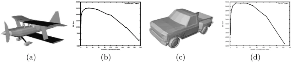
(d) Fig. 1. Two models from the database and their corresponding BIC Score curves.
Figure 1 shows the evolution of the BIC score with the number of views. Theses curves show that an optimal number of views exists where the BIC score is maximised. For the aeroplane model in figure 1(a), the number of optimal views is 29. For the car model in figure 1(c), only 17 views are needed as the 3D model is less complex then the first one. This is comming from the fact that the more the 3D model is geometrically complex, the more its 2D views are different. This leads to a higher number of views to best represent it.
4
Probabilistic approach for 3D indexing
Each model of the collection Db is represented by a set of characteristic views
V = {V1, V2, . . . , VC}, with C the number of characteristic views. To each
char-acteristic view corresponds a set of represented views called Vr. Considering a
3D request model Q, we wish to find the model Mi ∈ Db which is the closest
to the request model Q. This model is the one that has the highest probability P (Mi/Q). Knowing that each model is represented by its characteristic views,
P (Mi/Q) can be written: P (Mi|Q) = XC k=1P (Mi|V k Q)P (VQk|Q) . (4)
With C the number of characteristic views of the model Q. Let H be the set of all the possible hypotheses of correspondence between the request view Vk Q
and a model Mi, H = {hk1∨ hk2∨ . . . ∨ hkN}. A hypothesis hkp means that the view
p of the model is the view request Vk
Q. The sign ∨ represents logic or operator.
Let us note that if an hypothesis hk
p is true, all the other hypotheses are false.
P (Mi|VQk) can be expressed by P (Mi|Hk). We have:
P (Mi|Hk) = XN j=1P (Mi, V j Mi|h k j) . (5)
The sum PNj=1P (Mi, VMji|hkj) can be reduced to the only true hypothesis
P (Mi, V cjMi|H k
j). In fact, a characteristic view from the request model Q can
match only one characteristic view from the model Mi. We choose the
charac-teristic view with the maximum probability. P (Mi|Q) = XK k=1M axj(P (Mi, V j Mi|h k j))P (VQk|Q) . (6)
Using the Bayes theorem we obtain: P (Mi|Q) = K X k=1 M axj( P (hk j|V j Mi, Mi)P (V j Mi|Mi)P (Mi) PN i=1 PK k=1P (hkj|V j Mi, Mi)P (V j Mi|Mi)P (Mi) )P (Vk Q|Q) . (7) With P (M ) the probability to observe the model M .
P (Mi) = αe(−α.|Mi|)/
Pi=1
i=N|Mi|) . (8)
Where |Mi| is the number of characteristic views of the model Mi. α is a
parameter to hold the effect of the probability P (Mi). The algorithm conception
makes that, the more complex is the geometry of the 3D model, the greater is the number of its characteristic views. Indeed, simple object (e.g. a cube) are more frequent and got more probability of appearance then complex ones. This kind of object can be at the root of more complex objects.
On the other hand:
P (VMji|Mi) = 1 − βe(−β.N (V r j
Mi)/320) . (9)
Where N (V rjMi) is the number of views represented by the characteristic view j of the model M . The greater is the number of represented views N (V rjMi), the more the characteristic view VMji is important and the best it represents the three-dimensional model. The β coefficient is introduced to reduce the effect of the view probability. We use the values α = β = 1/100 which give the best results during our experiments.
The value P (hkj|V j
Mi, Mi) is the probability that, knowing that we observe
the characteristic view j of the model Mi, this view is the k view of the 3D query
model Q: P (hkj|V j Mi, Mi) = 1 − D(Qk,hVj Mi ) . (10) With Dhq,hVj Mi
the Euclidean distance between the 2D Zernike descriptors of the view k of the request model Q and VMji the characteristic view j of the three-dimensional model Mi.
In this section, we have presented our Bayesian retrieval framework, which takes into account the number of characteristic views of the model and the importance (amount of information) of its views. In the following section we present the results of experiments made by our method on Princeton 3D Shape Benchmark database [13].
5
Experiments and results
We implemented the algorithms, described in the previous sections, using C++ and the TGS OpenInventor libraries. The system consists in an off-line charac-teristic views extraction and an on-line retrieval process. In the off-line process,
the characteristic views selection takes about 18 seconds per model on PC with a Pentium IV 2.4 GHZ CPU. In the on-line process, the comparison takes less then 1 second for 1814 3D models. To measure the performance, we used a standard benchmark database: the Princeton 3D Shape Benchmark [13]. The database contain 1814 models manually classified into 161 classes.
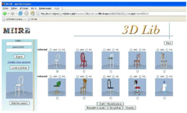
Fig. 2. Screenshot of the 3D models retrieval system.
Figure 2 shows a request using our 3D retrieval system. On the left side, the request 3D model is presented. The right side shows the 3D models which have the higher probabilities of matching the 3D request model. We use several dif-ferent performance measures to objectively evaluate our method: the First Tier (FT), Second Tier (ST), Nearest Neighbour (NN), E-Measure, Discounted Cu-mulative Gain (DCG) and Normalised Discounted CuCu-mulative Gain (N-DCG) match percentages, as well as the recall-precision plot [13]. As mentioned in the introduction, we compared our method to state of the art descriptors, Spheri-cal Harmonics [1], Radialized SpheriSpheri-cal Extent Function(REXT) [14], Gaussian Euclidean Distance Transform (GEDT) [1] and Light Field Descriptor (LFD) [6].
In our experiment, we use each of the five shape matching algorithms to compute distances between all pairs of models in the test and analyse them with the Princeton 3D Shape Benchmark evaluation tools to quantify the matching performance with respect to the classification.
Every model was normalised for size by isotropically rescalling it so that the average distance from points on its surface to the center of mass is 0.5. Then, all the models was normalised for translation by moving its center of mass to the origin.
Figure 3 shows the recall precision plots for our method AVC and the other shape descriptors. Table 1 shows micro averages storage requierement (for our method, we used 23 views that is the average number of views for all the database models) and retrieval statistics for each algorithm. Storage size is given in bytes. We found that micro and macro-average results gave consistent results, and we decided to present micro-averaged statistics.
We find that the shape descriptors based on 2D views (LFD and our method) provides the best retrieval precision in this experiment. We might expect shape
descriptors that capture 3D geometric relationships would be more discriminat-ing than the ones based solely on 2D projections, the opposite is true. However, our method and the LFD takes more time to compare than the other descriptors, since it requires searching over multiple possible image correspondances.
We can notice that our method provides more accurate results with the use of Bayesian probabilistic indexing. The experiment shows that our method gives better performances then 3D harmonics, Radialized Spherical Extent Function and Gaussian Euclidean Distance Transform on the Princeton 3D Shape Bench-mark database. Light Field Descriptor gives better results than our method but uses 100 views, does not adapt the number of views to the geometrical complexity and uses two descriptors for each view (Zernike moments and Fourier descrip-tor), which make it slower and more memory consuming descriptor compared to the method we presented.
Overall, we can conclude that our method gives a good compromise between quality (relevance) / cost (memory and online comparaison time) between the shape descriptors we compared to.
0 0.1 0.2 0.3 0.4 0.5 0.6 0.7 0.8 0.9 1 0 0.1 0.2 0.3 0.4 0.5 0.6 0.7 0.8 0.9 1 Precision Recall "LFD" "AVC" "REXT" "GEDT" "SHD"
Fig. 3. Recall Precision on Princeton 3D Shape Benchmark database.
Methods Discrimination
Storage size NN FT ST E-Measure DCG N-DCG
LFD 4,700 65.7% 38.0% 48.7% 28.0% 64.3% 21.3%
AVC with proba 1,113 60.6% 33.2% 44.3% 25.5% 60.2% 13.48%
REXT 17,416 60.2% 32.7% 43.2% 25.4% 60.1% 13.3%
GEDT 32,776 60.3% 31.3% 40.7% 23.7% 58.4% 10.2%
AVC without proba 1,113 58.2% 31.1% 42.7% 25.1% 59.9% 11,8%
Spherical Harmonics 2,184 55.6% 30.9% 41.1% 24.1% 58.4% 10.2%
Table 1. Retrieval performances.
In order to assess the robustness of our method, we apply the following transformations for all classified 3D models. Each transformed 3D model is then used to query the test database.
The average recall and precision of all the 1814 classified models are used for the evaluation (figure 5). The robustness is evaluated by the following transfor-mation:
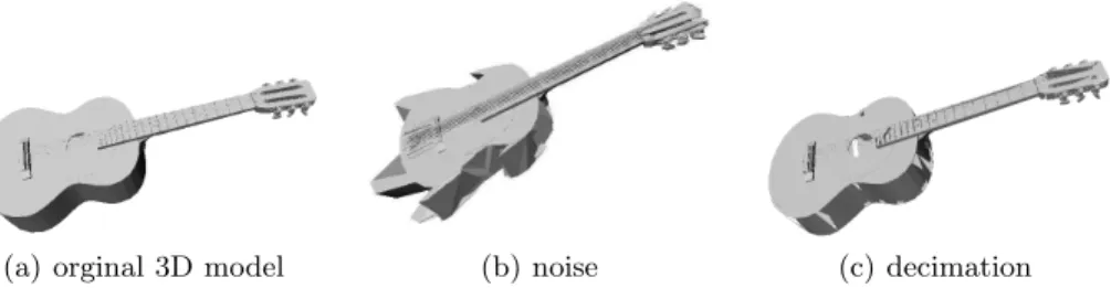
(a) orginal 3D model (b) noise (c) decimation Fig. 4. Robustness evaluation of noise and decimation from a 3D model.
1. noise: each vertex of 3D model is applied three random number to x-, y- and z-axis translation (±15% times of the length of the model’s bounding box). Figure 4(b) shows a typical example of the noise effect;
2. decimation: for each 3D model, randomly select 20% polygons to be deleted. Figure 4(c) shows a typical example of the effect.
Experimental results of the robustness evaluation is shown in Figure 5. These experimental results prove that our approach is robust against noise and deci-mation. 0 0.2 0.4 0.6 0.8 1 0 0.2 0.4 0.6 0.8 1 Precision Recall "Original" "Decimation" "Noise"
Fig. 5. Recall Precision on Princeton 3D Shape Benchmark database.
6
Conclusion
In this paper, we propose a 3D model retrieval system based on characteristic views similarity called AVC (Adaptive Views Clustering). Starting from the fact that the more the 3D model is geometrically complex, the more its 2D views are different, we propose a characteristic views selection algorithm that corresponds the number of views to its geometrical complexity. Our approach is based on alternating global k-means and adding new characteristic views where needed. The characteristic views set with the higher BIC score is choosed to represent the 3D model. The number of views varies from 1 to 40. We also propose a new probabilistic retrieval approach that takes into account that not all the views of 3D models have the same importance, and also the fact that geometrically simple models have more probability to be relevant than more complex ones. Based on
some standard measures, experiments and comparaison to some state of the art methods on Princeton 3D Shape Benchmark database, show the accurate results of our approach. The AVC method we proposed gives a good quality/cost com-promise compared to other well-known methods. Our method is robust against noise and model degeneracy. It can be suitable against topologically ill-defined 3D models. A practical 3D models retrieval system based on our approach will be soon available on the web for on-line tests.
7
Acknowledgments
This work is supported by the French Research Ministry and the RNRT (R´eseau National de Recherche en T´el´ecommunications) within the framework of the SEMANTIC-3D National Project (http://www.semantic-3d.net). We would like to thank Professor Dan Pelleg from Carnegie Mellon University for the help he provided on X-means, Julien Tierny and the reviewers for their help to make this paper more complete.
References
1. Kazhdan, M., Funkhouser, T., Rusinkiewicz, S.: Rotation invariant spherical
harmonic representation of 3d shape descriptors. In: Symposium on Geometric Processing. (2003)
2. Funkhouser, T., Min, P., Kazhdan, M., Haderman, A., Dobkin, D., Jacobs, D.: A search engine for 3D models. ACM Transactions on Graphics 22 (2003) 83–105 3. Cyr, C., B.Kimia: 3D object recognition using shape similarity-based aspect graph.
In: ICCV01. (2001) 254–261
4. Schiffenbauer, R.: A survey of aspect graphs. Technical Report TR-CIS-2001-01, CIS (2001)
5. Macrini, D., Shokoufandeh, A., Dickenson, S., Siddiqi, K., S.Zucker: View based 3-D object recognition using shock graphs. In: ICPR. Volume 3. (2002) 24–28 6. Chen, D., Tian, X., Shen, Y., Ouhyoung, M.: On visual similarity based 3D model
retrieval. In: Eurographics. Volume 22. (2003) 223–232
7. Tangelder, J., Veltkamp, R.: A survey of content based 3D shape retrieval methods. In: Shape Modeling International. (2004) 145–156
8. Khotanzad, A., Hong, Y.: Invariant image recognition by Zernike moments. IEEE Transactions on Pattern Analysis and Machine Intelligence 12 (90) 489 – 497 9. Duda, R., Hart, P.: Pattern classification and scene analysis. John Wiley and Sons
(1973)
10. Pelleg, D., Moore, A.: X-means: Extending k-means with efficient estimation of the number of clusters. In: International Conference on Machine Learning. (2000) 727–734
11. Schwarz, G.: Estimating the dimension of a model. The Annals of Statistics 6 (1978) 461–464
12. Akaike, H.: Information theory and extention of the maximum likehood principle. In: International symposium on information theory. (1973) 267–281
13. Shilane, P., Min, P., Kazhdan, M., Funkhouser, T.: The princeton shape bench-mark. In: Shape Modeling International. (2004)
14. Varnic, D.: An improvement of rotation invariant 3d shape descriptor based on functions on concentric spheres. In: ICIP. (2003) 757–760