Instrument-specific harmonic atoms for mid-level music representation
Texte intégral
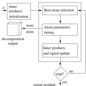
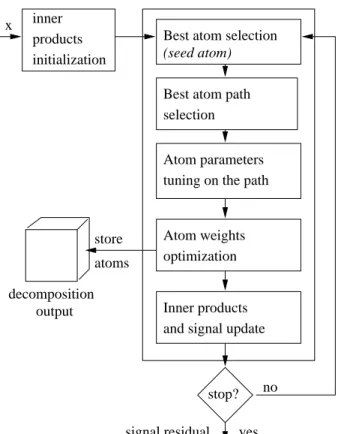
Figure
Documents relatifs
[38] made an analogy between image retrieval and text retrieval, and have proposed a higher-level representation (visual phrase) based on the analysis of visual word occurrences
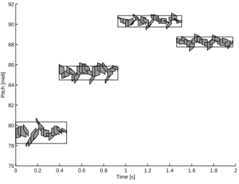
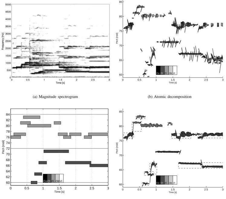
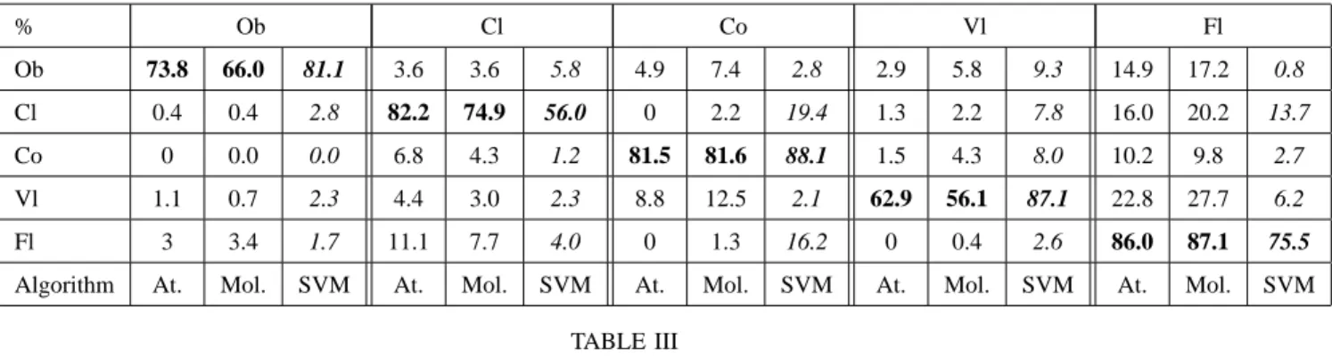
used as a mid-level representation of the mixture, displaying in our case its polyphonic pitch content, but also for applications such as melody extraction and lead
In this communication, starting from G-MUSIC which improves over MUSIC in low sample support, a high signal to noise ratio approximation of the G-MUSIC localization function is
Puis, nous avons étudié l’action d’une résonance de forme et des interférences à deux centres sur la phase spectrale, en montrant que dans le premier cas l’habillage de
fundamental musical element in his famous Traité de l'harmonie. Being absolutely fundamental for several tasks of analysis like the key determination, some additional information
Abstract - The Mossbauer Effect in 5 7 ~ e is used to discover and characterize chemical species formed between bare iron atoms or molecules with molecules of quasi-inert gases
In what follows we precise this notion and describe Niobé, a Common-Lisp-CLOS implementation of a system using PIMS for the specific case of generating musical sequences.... 4.1
emission of quanta of the external field are correlated in stimulated transitions, the gradient force is a regular quantity.. Spontaneous emission destroys the
