ILClass: Error-Driven Antecedent Learning For Evolving Takagi-Sugeno Classification Systems

(1)

HAL Id: hal-00881779

https://hal.archives-ouvertes.fr/hal-00881779

Submitted on 28 Jan 2014

HAL is a multi-disciplinary open access

archive for the deposit and dissemination of

sci-entific research documents, whether they are

pub-lished or not. The documents may come from

teaching and research institutions in France or

abroad, or from public or private research centers.

L’archive ouverte pluridisciplinaire HAL, est

destinée au dépôt et à la diffusion de documents

scientifiques de niveau recherche, publiés ou non,

émanant des établissements d’enseignement et de

recherche français ou étrangers, des laboratoires

publics ou privés.

ILClass: Error-Driven Antecedent Learning For

Evolving Takagi-Sugeno Classification Systems

Abdullah Almaksour, Eric Anquetil

To cite this version:

Abdullah Almaksour, Eric Anquetil.

ILClass:

Error-Driven Antecedent Learning For

Evolv-ing Takagi-Sugeno Classification Systems.

Applied Soft Computing, Elsevier, 2013, pp.1-16.

(2)

ILClass: Error-Driven Antecedent Learning For Evolving Takagi-Sugeno

Classification Systems

Abdullah Almaksour Eric Anquetil

IRISA - Intuidoc Team INSA de Rennes - France {abdullah.almaksour, eric.anquetil}@irisa.fr

Abstract

The purpose of this research work is to go beyond the traditional classification systems in which the set of recognizable categories is predefined at the conception phase and keeps unchanged during its operation. Motivated by the increasing needs of flexible classifiers that can be continuously adapted to cope with dynamic environments, we propose a new evolving classification system and an incremental learning algorithm called ILClass. The classifier is learned in incremental and lifelong manner and able to learn new classes from few samples. Our approach is based on first-order Takagi-Sugeno (TS) system. The main contribution of this paper consists in proposing a global incremental learning paradigm in which antecedent and consequent are learned in synergy, contrary to the existing approaches where they are learned separately. Output feedback is used in controlled manner to bias antecedent adaptation toward difficult data samples in order to improve system accuracy. Our system is evaluated using different well-known benchmarks, with a special focus on its capacity of learning new classes.

Keywords:

Evolving fuzzy classifiers, Online learning, Takagi-Sugeno, Classification

1. Introduction

Classification techniques represent a very active topic in machine learning. They appear frequently in many application areas, and become a basic tool for almost any pattern recognition task. Several structural and sta-tistical approaches have been proposed to build clas-sification systems from data. Traditionally, a classifi-cation system is trained using a learning dataset under the supervision of an expert that controls and optimizes the learning process. The system performance is funda-mentally related to the learning algorithm and the used learning dataset. The learning dataset contains labelled samples from the different classes that must be recog-nized by the system. In almost all learning algorithms, the learning dataset is visited several times in order to improve the classification performance which is usually measured using a separated test dataset. The expert can modify the settings of the learning algorithm and restart the learning process until obtaining an acceptable per-formance. Then, the classification system is delivered to the final user to be used in real applicative contexts. The role of the classifier is to suggest a label for each

un-labelled sample provided by the application. Typically, no learning algorithms are available at the user side.

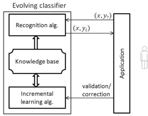
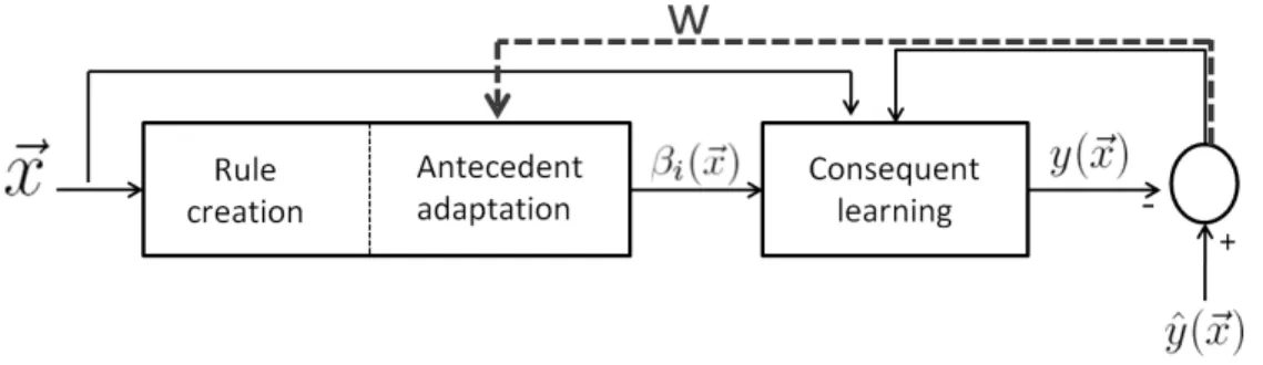
The main weakness in the above-mentioned concep-tion paradigm is that the knowledge base is constrained by the learning dataset available at expert side and can-not be extended by the data provided at user side. These drawbacks increase the need for new type of classifica-tion systems that can learn, adapt and evolve in lifelong continuous manner. As one can see from Figure 1, an incremental learning algorithm is used to learn from the data samples provided by the user after sending a valida-tion or a correcvalida-tion signal in order to confirm or change the label suggested by the classifier. Contrary to the tra-ditional paradigm, there is no separation between the learning phase and the operation phase in evolving clas-sification systems. One of the key features in evolving classifiers is that incoming samples may bring in new unseen classes that are learned by the classifier without destroying its knowledge base or forgetting the existing classes.

We have proposed in a previous work [1] an evolving Takagi-Sugeno (TS) classification system with an

(3)

im-Figure 1: Simultaneous operation and learning (incremental) pro-cesses in evolving classifiers

proved antecedent structure. It consists of a set of local linear regression models defined in different sub-spaces localized by the antecedent part of the rules. The rule-based structure of this system allows more flexibility in tuning its knowledge base, which makes it suitable for incremental learning. Recursive antecedent adaptation is coupled with a density-based incremental clustering to build the antecedent structure in the system. Con-sequent linear coefficients are estimated using recursive least squares method. The proposed learning algorithm has no problem-dependent parameters. In order to op-timize the system performance for classification prob-lems, a new method of antecedent learning in which out-put feedback is employed to supervise the re-estimation of prototype centers and covariance matrices. The goal is to focus on learning critical points and to improve the overall performance.

In this paper, we first reformulate and present in details the output-based antecedent learning method (called feed). Performance analysis of

ILClass-feed is then discussed and compared to the classic

statis-tical antecedent learning (called ILClass-stat). Contrary to ILClass-stat that behaves very well in the short term,

ILClass-feed has relative poor performance in the short

term, yet offering much better performance on the long term. Therefore, our effort in this paper is focused on proposing a new solution that combines the advantages of both ILClass-feed and ILClass-stat. The main criteria is to obtain the best possible performance for the short-and the long-term of learning. One can take for exam-ple the case of an evolving handwritten gesture classifier in which user defines his set of gestures providing few samples for each (short-term learning). It is very impor-tant in this example context to have a classifier with fast learning capacity. If user accepts the early system

per-formance, he would continue to use it providing more and more data samples (long-term learning).

Besides the focus on both early and late stages, a special emphasis is placed in this paper on the case of adding new classes to an existing classification system. The performance of our methods is studied in this con-text. It is important to mention that, to the best of our knowledge, it is the first work that evokes the problem of late learning of new classes by an evolving classifier. It can be also mentioned that very few works on evolving TS systems handle multiclass classification problems. Most of existing systems focus on prediction and regres-sion problems.

Before presenting our new evolving TS classifica-tion approach, we explain in Secclassifica-tion 2 the global struc-ture of TS systems and the different elements of most used incremental learning algorithms. We cite in the same section some known evolving TS systems. Our new system, called ILClass-hybrid is detailed in Sec-tion 3. Experimental validaSec-tion of the proposed system using well-known benchmark datasets is then presented in Section 4. Both synchronized and unsynchronized class learning is considered in our experiments.

2. Evolving Takagi-Sugeno (TS) systems: Overview

A Takagi-Sugeno system is defined by a set of fuzzy rules in which the antecedent part represents a fuzzy partitioning or clustering of the input space, and the out-put is calculated using a regression polynomial model over the input vector weighted by the antecedent acti-vation degree. Existing TS systems vary by their struc-ture (antecedent and consequent) or by the learning al-gorithms. A comparative table between several known TS systems is presented at the end of this section. In or-der to facilitate unor-derstanding of this table, the different structural and algorithmic elements used in TS systems are explained below.

2.1. TS architecture

As aforementioned, the structure of a TS system is divided into two parts: antecedent and consequent. We explain below the possible variants used in these two parts as well as the inference forward process in TS sys-tems.

2.1.1. Antecedent structure

Different types of membership functions can be used in TS models. The conjunction of the membership func-tions that are defined on the axes (features) of the input

(4)

space results in a hyper fuzzy zone of influence associ-ated to the fuzzy rule. The form of this fuzzy zone is re-lated to the used membership function of the antecedent part.

Considering the case of Gaussian functions, one can rewrite the fuzzy rules of TS models so that the an-tecedent part is represented by a fuzzy zone of influence with hyper-spherical shape. This zone of influence can be characterized by a center and a radius value. In the rest of this paper, the word “prototype” will be used to refer to the fuzzy zone of influence of a fuzzy rule.

In data-driven design of TS models, the antecedent of fuzzy rules are formed using batch or incremental fuzzy clustering methods over a learning data set. These clustering methods aim at finding the prototypes’ cen-ters and estimating the radius value in order to optimally cover the input data cloud(s).

The firing degree of the antecedent part can be ex-pressed by a specific distance that represents the close-ness degree between the input vector and the fuzzy pro-totype (equation 1).

Rulei: IF ~x is close to Pi THEN y1i = l 1 i(~x), ..., y k i = l k i(~x) (1) where Pi represents the fuzzy prototype associated to

the rule i, k represents the number of classes and lm_i(~x) is the linear consequent function of the rule i for the class m.

For spherical [2] or axes-parallel hyper-elliptical [3] prototypes, the firing degree can be com-puted depending on the prototype center ~µiand the

ra-dius value σi(the same value in all the dimensions for

the former, and different values for the latter). In our model [1], we went a step ahead in the structure of the antecedent part of TS models. In addition to the use of different variance values in the definition of the fuzzy prototypes in the input data space, the covariance be-tween the features is taken into consideration. There-fore, the fuzzy influence zone of each rule is represented by a prototype with a rotated hyper-elliptical form. Each fuzzy prototype in our system is yet represented by a center ~µiand a covariance matrix Ai:

Ai=               σ2 1 c12 ... c1n c21 σ2 2 ... c2n ... ... ... ... cn1 cn2 ... σ2n               i (2)

where c12(= c21) is the covariance between x1and x2,

and so on.

Different multi-dimensional (multivariate) probabil-ity densprobabil-ity functions can be used to measure the activa-tion degree of each prototype. The most used ones are:

• Multivariate normal distribution: the activation is

calculated according to this distribution as follows:

βi(~x) = 1 (2π)n/2_|A i|1/2 exp ₋1 2(~x − ~µi) t_A−1 i (~x − ~µi) ! (3)

• Multivariate Cauchy distribution: the activation

here is defined as follows:

βi(~x) = 1 2π√_|Ai| h 1 + (~x − ~µi)tA−1i (~x − ~µi) i−n+1₂ (4) After an experimental comparative study on different benchmark datasets, it had been concluded that mul-tivariate Cauchy distribution slightly outperforms the Normal distribution. However, the presented learning algorithm is independent of this choice, and the applied distribution has no effect on the manner of estimation of variance/covariance matrices. Cauchy distribution is used in our experiments.

2.1.2. Inference process

When using TS models in a classification problem, the inference process, applied to get the class of a given input vector ~x, consists of three steps:

• The activation (or firing) degree of each rule βi(~x)

in the model is calculated (using equation 4, for example). It must then be normalized as follows:

¯ βi(~x) = βi(~x) Pr j=1βj(~x) (5)

where r represents the number of rules in the model.

• the sum-product inference is used to compute the

system output for each class:

ym(~x) = r X i=1 ¯ βi(~x)ymi (6)

where ym_i = lm_i (~x) is the consequence part of the rule i related to the class m.

• The winning class label is given by finding the

maximal output and taking the corresponding class label as response:

class(~x) = y = argmax ym(~x) m = 1, .., k

(5)

2.1.3. Consequence variants

Three different consequent structures can be used in TS models: binary, singleton [4] or polynomial [5] [2] [6] [1]. The latter is the more sophisticated form used in TS models in order to achieve higher precision. The focus will be placed on first-degree linear consequent. Models with such consequent structure are called “First-order TS models”. Thus, the linear consequent function is written as follows: lm_i(~x) = ~πm i ~x = a m i0+ a m i1x1+ a m i2x2+... + a m inxn (8) where lm

i(~x) is the linear consequent function of the rule i for the class m.

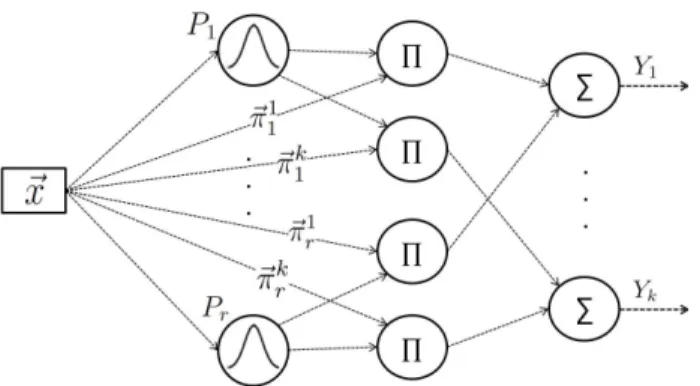
It had been proved that zero-order TS models are functionally equivalent to the well-Radial Basis Func-tion Networks (RBFN) [7]. The structures of these two models can be compared so that fuzzy prototypes in TS models are equivalent to the hidden neurons in RBFN, and singleton consequences in TS models are equivalent to the weights in RBFN between the hidden and the out-put layer. For the purpose of comparison between first-order and zero-first-order TS, Figure 2 shows a first-first-order TS model in the form of an RBF network with a second hidden layer.

2.2. TS Incremental Learning

Let’s suppose xi, i = 1, 2, .., n represent the

learn-ing data samples, M refers to the learned system, and

f refers to a given learning algorithm. Then, the

dif-ference between batch and incremental learning can be simply defined as follows:

Batch: Mi= f (x1, x2, .., xi)

Incremental: Mi= f (Mi−1, xi)

We focus in this section (and all along the paper) on incremental learning algorithms. Batch learning of TS systems is beyond the scope of this paper.

2.2.1. Rule creation

The focus is placed on incremental clustering be-cause our classifier is based on fuzzy rule-based sys-tem, in which rule creation is usually considered as a clustering problem. In incremental clustering, each new point may either reinforce an existing cluster, and eventually changes its characteristics (i.e. its center and zone of influence), or trigger the creation of a new clus-ter. The main difference between incremental clustering methods is the criterion used to make the decision be-tween these two choices. According to this criterion, we can categorize incremental clustering methods into distance-based and density-based methods.

Most of existing TS models use distance-based in-cremental clustering [4] [5] [2]. In these methods, a threshold value is directly or indirectly defined and used to decide whether a new cluster must be created or not depending on the minimum distance between the new data point and the existing cluster centers. Some exam-ples of these methods are ART Networks [8], VQ and its extensions [9] [10], ECM [5], etc. The main draw-back of these methods is the strong dependence on the minimum inter-clusters threshold value. A bad setting of this threshold may lead to either over-clustering (a data cluster is divided into several small ones), or under-clustering (different clusters are erroneously merged to form one big cluster). Another major disadvantage of distance-based incremental clustering is the sensibil-ity to noise and outlier points. Therefore, we believe that density-based techniques are much more suitable for incremental clustering. Contrary to distance-based ones, density-based techniques do not depend on an ab-solute threshold distance to create new cluster. They rely on density measures to make a global judgement on the relative data distribution. The representativity of a given sample in a density-based clustering process can be evaluated by its potential value. The potential of a sample is defined as inverse of the sum of distances be-tween a data sample and all the other data samples [11]:

Pot(~x(t)) = 1

1 +Pt−1

i=1kx(t) − x(i)k

2 (9)

A recursive method for the calculation of the poten-tial of a new sample was introduced in [6] under the name of eClustering method. The recursive formula avoids memorizing the whole previous data but keeps -using few variables - the density distribution in the fea-ture space based on previous data. The potential of each new instance is thus estimated as follows:

Pot(~x(t)) = t − 1 (t − 1)α(t) + γ(t) − 2ζ(t) + t − 1 (10) where α(t) = n X j=1 x2_j(t) (11) γ(t) = γ(t − 1) + α(t − 1), γ(1) = 0 (12) ζ(t) = n X j=1 xj(t)ηj(t), ηj(t) = ηj(t−1)+xj(t−1), ηj(1) = 0 (13) Introducing a new sample affects the potential values of the centers of existing clusters, which can be recursively

(6)

Figure 2: First-order TS model presented as a neural network

updated by the following equation:

Pot(µi) = (t − 1)Pot(µ

i)

t − 2 + Pot(µi) + Pot(µi)Pnj=1kµi− x(t − 1)k2_j

(14) If the potential of the new sample is higher than the po-tential of the existing centers then this sample will be a center of a new cluster. The potential value of such new center is initialized by 1. This density-based method had been first used for TS systems in [6]. Our system in [1] uses eClustering. Given that our focus here is placed on supervised incremental learning for classifi-cation problems, we can suppose that the addition of new classes can be explicitly pointed out by an external signal. A new rule is automatically created in our sys-tem for the first data sample from a new class. For the next samples, eClustering is used to detect the emer-gence of new regions with relative high data density. The data point ~xtthat triggered the creation of new rule

(new class or new region of interest) is considered as prototype center ( ~µr+1 = ~xt). An initial diagonal

vari-ance/covariance matrix is associated to the new proto-type. The initial diagonal values are estimated as the average diagonal values of existing prototypes.

2.2.2. Antecedent adaptation

The antecedent of each fuzzy rule in a FIS is repre-sented by a prototype in multidimensional space, and this prototype can have different shapes (hyper-boxes, hyper-spheres, etc.). While creating new prototypes is done using incremental clustering as explained in the precedent section, the parameters of prototype position and shape should be continuously and incrementally re-estimated in evolving FIS in order to get an up-to-date representation. Antecedent adaptation technique depends on prototype shape. It can be generally di-vided into two steps: prototype position displacement, and prototype zone of influence re-estimation (box

ex-panding in [4], radius update in [3], etc.). In our system [1], prototype centers are shifted and their covariance matrices are updated according to incoming samples.

2.2.3. Consequece learning

Weighted Recursive Least Squares method is used in most TS systems for learning consequent parameters in online manner. It is explained below how this method is used for TS consequent recursive estimation.

Coefficient estimation of TS consequent functions can be seen as a problem of solving a system of linear equations expressed as follows:

(Ψi +δI)Π = Yi i = 1, 2, ..., t1 (15)

where Π is the matrix of all the parameters of system linear consequences. Π =               ~π1 1 ~π 2 1 ... ~π k 1 ~π1 2 ~π 2 2 ... ~π k 2 ... ... ... ... ~π1 r ~π2r ... ~πkr              

k represents the number of classes and r is the number

of fuzzy rules,

Ψi = [β1(~xi)~xi, β2(~xi)~xi, ..., βr(~xi)~xi] is the input vector

(a vector of real values representing the input features) weighted by the activation degrees of prototypes, and

Yiis the ground truth output vector (a vector of binary

values in classification problems). In order to stabi-lize and to smooth the solution, a regularization term

δ (known as Tychonoff regularization) is added to the

equation. Solving this system of linear equations by the least squares method consists in minimizing the next

1_{It is worth mentioning that the term t in this paper has no temporal} meaning. Given that the system is fed in discrete manner, t is only incremented at the arrival of a new data.

(7)

cost function: E = t X i=1 kΨiΠ − Yik2+ω kΠk2 (16)

where ω = δ2_{is a positive number called the}

regulariza-tion parameter, and I is the identity matrix. The soluregulariza-tion that minimizes the cost function of Equation 16 is:

Πt= ( t X i=1 ΨiΨTi +ωI)−1. t X i=1 ΨiYi (17)

We rewrite Equation 17 by replacing (Pt

i=1ΨiΨT_i +ωI)

and (Pt

i=1ΨiYi) by Φtet Zt, respectively:

Πt= Φ−1t .Zt (18)

By isolating the term corresponding to i = t, one can rewrite Φtas follows: Φt=         t−1 X i=1 ΨiΨTi +ωI         + ΨtΨTt (19)

Thus, the matrix Φ is updated using the following recur-sive formula:

Φt= Φt−1+ ΨtΨTt (20)

In the same way, a recursive formula to update the ma-trix Z can be deduced :

Zt= Zt−1+ ΨtYt (21)

In order to calculate Πtusing Equation 18, Φ−1t need

to be calculated. This can be done using the following lemma:

Lemma 1 : Let A = B−1+ CD−1CT, the inverse of A is given as follows:

A−1_{= B − BC(D + C}TBC)−1CTB (22)

To apply Lemma 1 on Equation 20, we make the fol-lowing substitutions:

A = Φt, B−1= Φt−1, C = Ψt, D = 1

Thus, the recursive formula of the inverse of the matrix

Φ can be obtained as follows: Φ−1_t = Φ−1_t−1₋Φ

−1

t−1ΨtΨTt Φ−1_t−1

1 + ΨTt Φ−1_t−1Ψt

(23)

Π is then calculated as next:

Πt = Φ−1t Zt= Φ−1t (Zt−1+ ΨtYt) = Φ−1_t (Φ_t−1Π_t−1+ ΨtYt) = Φ−1_t ((Φt− ΨtΨTt)Πt−1+ ΨtYt) = Π_t−1_{− Φ}−1t ΨtΨtTΠt−1+ Φ−1t ΨtYt

= Π_t−1_{− Φ}−1_t Ψt(Yt− ΨTt Πt−1) (24)

The initialization of the algorithm consists in deter-mine two quantities:

• Π0 : In practice, and when no prior knowledge is

available, Π0is initialized by 0.

• Φ−1

0 : Given Φt= Pt

i=1ΨiΨT_i +ωI and by putting t

equals 0, we find that Φ−1₀ =ω−1_{I, where ω is the}

regularization parameter.

Large values of ω−1 _{(between 10}2 _{and 10}4_{) are}

gener-ally adopted when signal-to-noise ratio on input vec-tor is high, which is the case in our system especially at the beginning of learning where significant modifica-tions are applied on the prototypes. The impact of ω−1 value according to input noise level is discussed in [12]. When a new rule is created, its parameters are initialized by the average of the parameters of other rules:

Πt=                      ~π1 1(t−1) ~π 2 1(t−1) ... ~π k 1(t−1) ~π1 2(t−1) ~π 2 2(t−1) ... ~π k 2(t−1) ... ... ... ... ~π1 r(t−1) ~π 2 r(t−1) ... ~π k r(t−1) ~π1 (r+1)t ~π 2 (r+1)t ... ~π k (r+1)t                      (25) where ~πc (r+1)t= r X i=1 βi(~xt)~πc_i(t−1) (26)

The matrix Φ−1_{is extended as follows:}

Φ−1_t =                      ρh Φ−1 t−1 i h 0 i h 0 i           Ω−1 _... ₀ ... ... ... 0 ... Ω−1                                (27)

where ρ = (r2 _{+ 1)/r}2_{. This recursive least squares}

(RLS) consequent learning is used in most TS systems.

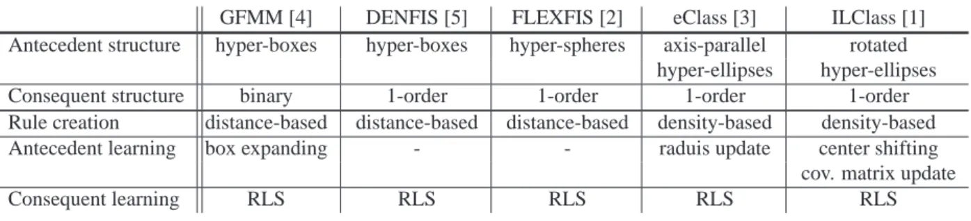
We sum up the main features of the evolving TS sys-tems mentioned in this section in Table 1.

It can be noticed that the antecedent is learned inde-pendently from the consequent learning in the above-mentioned systems. However, few other approaches propose a global learning of fuzzy rule-based models.

The authors of [13] proposed an extension of the classic neural networks error back-propagation method based on the gradient descent called ANFIS (Adap-tive Neuro-Fuzzy Inference Systems). In this exten-sion, a hybrid learning method that combines the gradi-ent method and the least squares method is used. Each

(8)

GFMM [4] DENFIS [5] FLEXFIS [2] eClass [3] ILClass [1] Antecedent structure hyper-boxes hyper-boxes hyper-spheres axis-parallel rotated

hyper-ellipses hyper-ellipses

Consequent structure binary 1-order 1-order 1-order 1-order

Rule creation distance-based distance-based distance-based density-based density-based Antecedent learning box expanding - - raduis update center shifting

cov. matrix update

Consequent learning RLS RLS RLS RLS RLS

Table 1: A comparison table between existing evolving TS systems

epoch of this hybrid learning procedure is composed of a forward pass and a backward pass. In the forward pass, the parameters (weights) in the output layer are identified using the least squares estimation. Then, the error rates propagate from the output toward the input end and parameters in the hidden layer(s) are updated the gradient descent method. Based on the functional equivalence between adaptive networks and fuzzy in-ference systems, the hybrid learning method is used to learn a fuzzy inference system of Takagi Sugeno’s type. Thus, consequent parameters are first estimated using least squares, and premise parameters are then updated using error-propagation gradient descent. Despite the wide use of ANFIS in different applications, we can note that it cannot be used in an evolving learning con-text because of its fixed structure. However, it is still a robust learning algorithm for adaptive classification sys-tems.

EFuNN (Evolving Fuzzy Neural Networks) [14] is a fuzzy rule-based classification system in which each rule represents an association between a hypersphere from the fuzzy input space and a hypersphere from the fuzzy output space. The pair of fuzzy input-output data vectors (xf, yf) is allocated to a rule ri if xf falls in

the input hypersphere and yf falls in the output

hyper-sphere. The former condition is directly verified using a local normalized fuzzy distance, whereas the latter is indirectly verified by calculating the global output error. EFuNN algorithm starts by evaluating the local normal-ized fuzzy distance between the input vector and the ex-isting rules in order to calculate the activations of the rule layer. The activation of the fuzzy output layer is calculated based on the activations of input layer and the centers of hyperspheres in output layer. The cen-ters of input hyperspheres are adjusted depending on the distance between the input vector and rule nodes, and centers of output hyperspheres are also adapted using a gradient descent. However, a supervised adaptation of the input hyperspheres centers is also possible based on

a one-step gradient descent method. Although EFuNN structure has been presented differently, it is function-ally equivalent to Mamdani fuzzy inference system. The distance-based incremental clustering method used in EFuNN in both input and output space depends strongly on the sensitivity threshold.

3. Antecedent learning optimization in evolving Takagi-Sugeno classifiers

As mentioned before, we proposed in [1] an evolv-ing TS classification system with first-order consequent structure. We used an enhanced antecedent structure so that each prototype is represented by a center and a co-variance matrix.

Incremental learning of TS models is generally di-vided into two independent learning processes: an-tecedent learning and consequent learning. This work focuses on finding an optimal antecedent structure that can improve the overall system performance.

Antecedent learning can be simply done in straight-forward recursive statistical manner so that prototype center and covariance matrix are re-estimated after each new data sample in order to give it the rotated hyper-elliptical form. All samples have the same weight and antecedent structure is built in unsupervised way; i.e. system output is not considered in the learning pro-cess. Our system with this simple method will be called

ILClass-stat and presented in section 3.1.

Looking for new techniques that optimize antecedent structure and enhance system performance, we pre-sented in [1] a global learning paradigm for evolving TS classifiers. The core idea of this paradigm is to learn the antecedent and the consequent part in correlated mner so that the output error is used to supervise the an-tecedent learning process. The goal of this supervision is to focus learning on samples with high output error and thus to reduce misclassification errors. To the best

(9)

of our knowledge, this is the first system in which out-put feedback is employed in antecedent learning. This approach is called ILClass-feed and explained in sec-tion 3.2.

Although ILClass-feed had shown good results [1] by improving the long-term system accuracy for several in-cremental classification problems, it had been system-atically outperformed by ILClass-stat in the short-term (at the beginning of learning process where only few data are available). The main purpose of this paper is to cope with this problem by proposing a new solution that can be efficient during the whole learning process, i.e. good performance at the early learning stage cou-pled with the best possible long-term performance. This new solution will be explained in section 3.3 and called

ILClass-hybrid.

3.1. ILClass-stat: statistical antecedent learning

For each new sample ~xt, the center and the covariance

matrix of the prototype that has the highest activation degree are updated.

The recursive estimation of the center can be found as follows:

~

µt= (1 − α) ~µt−1+ α ~xt (28)

α =1

t (29)

where t represents the number of updates that have been applied so far on this prototype.

The covariance matrix can be recursively computed as follows:

At= (1 − α) At−1+ α (~xt− ~µt)(~xt− ~µt)T (30)

All incoming samples are treated equitably in the above formulas that are straightforward statistical mean and covariance calculations.

3.2. ILClass-feed: antecedent learning driven by out-put feedback

The fundamental idea of the novel approach is to use an output error feedback in the antecedent adaptation (as illustrated in Figure 3), contrary to existing approaches where the antecedent is learned independently from the consequent learning and the overall output. The pur-pose of integrating the output signal in the antecedent learning is to bias it towards the incoming points with high output error so that the more the error is high the more will be the influence of this point on the antecedent adaptation. Thanks to this improvement, it becomes possible in the antecedent adaptation to focus on the

data points that are misclassified by the system or hardly well-classified, and to put less focus on non-problematic points.

To formulate this concept, we introduce in the an-tecedent adaptation formulas a weight value calculated for each sample so that α is calculated as follows:

α = wt wcumul (31) wcumul= t X i=1 wi (32)

where w represents the “weight” associated to the data point ~xt. The value of w is related to the output error

committed by the system for the current point ~xt.

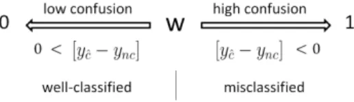
In classification problem, the quality is perceived by the user from the number of misclassification er-rors committed by the system. The value of w can be calculated so that it becomes higher for points with a high risk of misclassification. The risk of misclassifi-cation of each sample is estimated by its confusion de-gree. The confusion degree is inversely proportional to the difference between the score of the true class of ~x, and the highest score within the other (wrong) classes. The confusion-driven antecedent learning is then imple-mented by calculating w for each incoming sample as follows:

w = (1 − [yˆc− ync])/2 w ∈ [0, 1] (33)

where yˆc is the system output corresponding to ˆc that

represents the true class of ~xt, and

ync= argmax yc ; c = 1...k & c , ˆc (34)

The value of w tends toward 0 when ~xt is “strongly”

recognized, and toward 1 when it is misrecognized. The risk of misclassification associated to ~xtis proportional

to the confusion degree estimated by the value of w. (see Figure 4)

Figure 4: Confusion degree estimation (W for error samples is greater than 0.5, and less than 0.5 for recognized ones)

System quality in regression and time-series predic-tion problems is related to the difference between sys-tem output vector and real output vector, and can be

(10)

Figure 3: ILClass-feed learning paradigm: antecedent adaptation driven by output feedback

measured using different indications. w can be calcu-lated in these cases by the distance between system out-put vector ~y and ground truth vector ˆ~y (contains 1 for the

true class and 0s for the rest). Thus, the value of w can be estimated as follows: w =1 2 k X c=1 | ˆyc− yc| (35)

where k is the number of classes. The proposed idea can be implemented using different quality measures, like R-squared adjusted [2], non-dimensional error in-dex (NDEI) [5], or normalized RMSE [6]. However, the focus in this paper is placed on classification prob-lems and the confusion-based calculation (Equation 33) will be employed all along the experimental section.

3.3. ILClass-hybrid: ILClass-stat/ILClass-feed error-based sliding

As explained above, ILClass-feed uses system scores to estimate the weight of each sample. Antecedent structure is then highly influenced by system perfor-mance. When experimenting it, ILClass-feed was able to outperform ILClass-stat after a specific period of in-cremental learning. Nevertheless, results have shown the relatively poor performance of ILClass-feed at the early phase of learning so that it is always beaten by ILClass-stat method. Figure 5(a) (using PenDigits dataset) illustrates this phenomenon and the intersection point of the two curves. These results can be explained by the system instability at the beginning of learning where only few data samples are learned and important fluctuations appear at system output during this early stage. Therefore, antecedent learning in ILClass-feed will suffer from this instability and need a period of time to reach its expected good performance. The more sys-tem output gets stable, the more ILClass-feed can en-hance its performance, as shown in Figure 5(a). On the other hand, ILClass-stat copes well at the early stage al-lowing a stable statistical prototype initialization, but its

1 2 3 4 5 6 7 500 1000 1500 2000 2500 3000 3500 4000 Misclassification rate (%)

Number of learning samples Evolve-stat Evolve-feed (a) 1 2 3 4 5 6 7 500 1000 1500 2000 2500 3000 3500 4000 Misclassification rate (%)

Number of learning samples Evolve-stat Evolve-feed Desired solution

(b)

Figure 5: (a) Performance curve intersection between ILClass-stat and ILClass-feed (b) The optimal looked-for performance

performance stagnates for the long term. It is worth re-minding that achieving acceptable early performance is mandatory in many applications where user is involved in the learning cycle.

An ideal solution consists then in proposing a new method that profits of the advantage of ILClass-stat for the short term, and that of ILClass-feed for the long term. The objective is to get the performance illustrated by the black curve in Figure 5(b).

To cope with this problem, we propose a new ap-proach, called ILClass-hybrid, that allows a gradual sliding between ILClass-stat and ILClass-feed. It is worth reminding that one of the main criteria in the learning algorithm is to be completely free of problem-depended parameters. Thus, the sliding mechanism

(11)

from ILClass-stat to ILClass-feed is automatically con-trolled by a system stability measure represented by λ, as follows: α = λ1 t + (1 − λ) wt wcumul (36) λ = nbErr t λ ∈ [0, 1] (37)

where nbErr is the accumulated number of misclassifi-cation committed on the incoming samples. Early val-ues of λ are close to 1 because of the high number of error at the beginning of incremental learning process. Then, its value tends more-or-less rapidly towards small values close to 0. Using Equation 36, ILClass-hybrid automatically adjusts the combination of ILClass-stat and ILClass-feed according to the relative error level observed at system output.

Thus, the formulas used in ILClass-hybrid can be summed up as follows: ~ µt= (1 − α) ~µt−1+ α ~xt At= (1 − α) At−1+ α (~xt− ~µt)(~xt− ~µt)T α = λ 1 t + (1 − λ) wt wcumul λ = nbErr t λ ∈ [0, 1] wt= (1 − [yˆc− ync])/2 w ∈ [0, 1] ync= argmax yc ; c = 1...k & c , ˆc wcumul= t X i=1 wi 4. Experimental Validation

Experiments in this paper will be mainly focused on studying the performance of ILClass-hybrid as an op-timal compromise between stat and

ILClass-feed. The three models are evaluated for different incremental classification problems using benchmark datasets. Short- and long-term performance compar-isons between the three models are presented in this sec-tion.

In addition to the validation of ILClass-hybrid, we present in this section another original point of this pa-per that consists in studying the behaviour of an evolv-ing TS classifier when addevolv-ing new unseen classes to the system. In this novel evaluation scenario, the aim is to examin the system reaction to the addition of new classes, and to test its performance recovery speed.

The benchmark datasets used in our tests are first pre-sented, then some details about our experimental proto-col are given. Results are then presented and divided into two parts: results for synchronized class learning, and results for unsynchronized class adding.

4.1. Classification datasets

We evaluate our algorithms on several well-known classification benchmarks form the UCI machine learn-ing repository [15]. We followed two criteria in select-ing the datasets :

• They should represent multiclass problems. Our

learning algorithms are optimized for classification problem with more than two classes.

• The number of samples per class in each dataset

should be large enough for two reasons. The first is to have a large learning dataset that allows contin-uing the incremental learning as far as possible and to examine the behaviour of the algorithms in the long term. The second reason is to have a large test dataset to be able to correctly evaluate the classi-fier during the incremental learning process as seen later. The large size of the test dataset helps as well to neutralize as much as possible the order effect on the results.

Respecting the last two criteria, the next datasets had been chosen from UCI machine learning repository to be used in our experiments:

• CoverType: The aim of this problem is to predict

forest cover type from 12 cartographical variables. Seven classes of forest cover types are considered in this dataset. A subset of 2100 instances is used in our experiments.

• PenDigits: The objective is to classify the ten

dig-its represented by their handwriting information from pressure sensitive tablet PC. Each digits is represented by 16 features. The dataset contains about 11000 instances.

• Segment: Each instance in the dataset represents

a 3x3 region from 7 outdoor images. The aim is to find the image from which the region was taken. Each region is characterized by 19 numerical at-tributes. There are 2310 instances in the dataset.

• Letters: The objective is to identify each of a large

number of black-and-white rectangular pixel dis-plays as one of the 26 capital letters in the English alphabet. Each letter is represented by 16 primitive

(12)

Dataset # Classes # Features # Instances CoverType 7 54 2100 PenDigits 10 16 10992 Segment 7 19 2310 Letters 26 16 20000 JapaneseVowels 9 14 10000

Table 2: Characteristics of learning datasets

numerical attributes. The dataset contains 20000 instances.

• JapaneseVowels: The goal is to distinguish nine

male speakers by their utterances of two Japanese vowels. Each vector is characterized by 14 values. The dataset contains 10000 samples.

The characteristics of the five datasets are summa-rized in Table 2. The five datasets used in our exper-iments vary by both the number of features (number of data space dimensions), and the number of classes, which allows testing our algorithms on different multi-class problems.

4.2. Experimental protocol

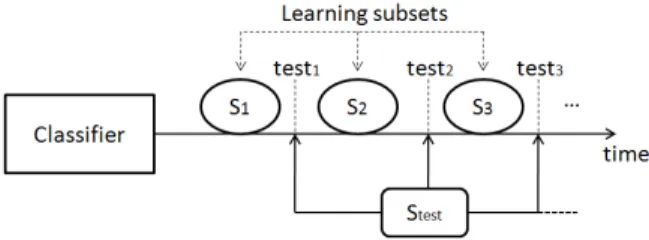
Figure 6: Periodic held-out evaluation protocol

A repeated 10-folds cross-validation (CV) data parti-tioning protocol is employed in our experiments. For each CV, the samples of training subset (90% of en-tire dataset) are sequentially introduced to the system in 10 different random orders. Thus, experiment for each dataset is repeated 100 times and average results are presented in the figures below. The test subset is used to estimate the recognition rate achieved by the classifier during the incremental learning process. The term “learning subset” is used to identify the group of instances learned by the system between each two con-secutive tests. When a new class appears in a given learning subset Si, test samples of the same class are

added to the test subset Stest. After learning each new Si, a new evaluation point is estimated using Stest and

the curves drawn in the next figures represent an inter-polation of these points. This incremental learning pro-tocol is called periodic held-out propro-tocol. (Figure 6)

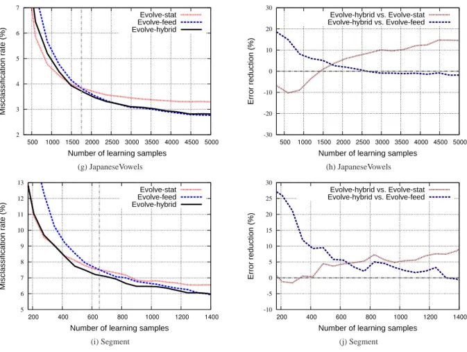
4.3. Results for synchronized classes

We present in Figure 7 the results of the three mod-els for five different benchmark datasets. In these fig-ures, the evolution of the generalization misclassifica-tion rate of the three models is presented, from the very beginning of the incremental learning process (few sam-ples per class), until a relatively advanced learning state (limited by the size of the used datasets). We show in the same figures the relative reduction of misclassi-fication rate achieved by ILClass-hybrid compared to

ILClass-stat and ILClass-feed. All classes in this first

part of experiments are introduced to the system in quasi-synchronized manner (random sample orders are applied without any constraint on sample classes).

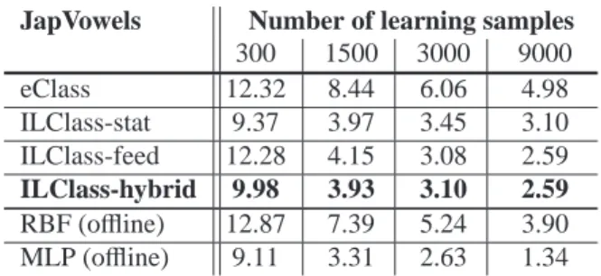
The obtained results are also synthesized in Tables 3-7 where the performance is measured at four different moments of incremental learning (i.e. different num-ber of learned samples) that represent short-term and long-term viewpoints. In addition to the ILClass-stat,

ILClass-feed and ILClass-hybrid, the performance

ob-tained by the evolving TS approach eClass [3] is given in the tables. Besides, we present in the same tables the misclassification rates obtained by two batch classifiers: radial basis function (RBF) classifier and multilayer per-ceptron (MLP, one hidden layer with 10 neurons). The implementation of these two classifiers is provided by Tanagra software.

The obtained results confirm the analysis given in Section 3.3 about the difficulties that face ILClass-feed in the early learning phases due to high perturbation of antecedent learning. Nonetheless, they approve the con-siderable gain of performance that can be achieved by

ILClass-feed in the long term, compared to ILClass-stat

method.

More importantly, results show the very good per-formance of ILClass-hybrid that almost covers the op-timal combined performance obtained by ILClass-stat end ILClass-feed at both short- and long-term learning moments. It can be noted that ILClass-hybrid allows in average about 15% of error reduction when compared to ILClass-feed at the early stage of learning. This size-able gain is very important in many application con-texts in which online incremental learning is required to be sufficiently fast. The short-term performance can play a key role in user acceptance of evolving classi-fiers. The short-term enhancement in ILClass-hybrid does not sacrifice the good performance of the output feedback model (ILClass-feed) and ILClass-hybrid also achieves about 15% of error reduction when compared to ILClass-stat after a long-term incremental learning.

(13)

1 1.5 2 2.5 3 3.5 4 4.5 5 500 1000 1500 2000 2500 3000 3500 4000 4500 5000 Misclassification rate (%)

Number of learning samples

Evolve-stat Evolve-feed Evolve-hybrid (a) PenDigits -10 0 10 20 30 40 50 500 1000 1500 2000 2500 3000 3500 4000 4500 5000 Error reduction (%)

Evolve-hybrid vs. Evolve-stat Evolve-hybrid vs. Evolve-feed (b) PenDigits 10 12 14 16 18 20 2000 3000 4000 5000 6000 7000 8000 Misclassification rate (%)

Evolve-stat Evolve-feed Evolve-hybrid (c) Letters -10 -5 0 5 10 15 20 25 2000 3000 4000 5000 6000 7000 8000 Error reduction (%)

Evolve-hybrid vs. Evolve-stat Evolve-hybrid vs. Evolve-feed (d) Letters 14 16 18 20 22 24 26 28 30 200 400 600 800 1000 1200 1400 1600 Misclassification rate (%)

Evolve-stat Evolve-feed Evolve-hybrid (e) Cover -30 -20 -10 0 10 20 30 200 400 600 800 1000 1200 1400 1600 Error reduction (%)

Evolve-hybrid vs. Evolve-stat Evolve-hybrid vs. Evolve-feed

(14)

2 3 4 5 6 7 500 1000 1500 2000 2500 3000 3500 4000 4500 5000 Misclassification rate (%)

Evolve-stat Evolve-feed Evolve-hybrid (g) JapaneseVowels -30 -20 -10 0 10 20 30 500 1000 1500 2000 2500 3000 3500 4000 4500 5000 Error reduction (%)

Evolve-hybrid vs. Evolve-stat Evolve-hybrid vs. Evolve-feed (h) JapaneseVowels 5 6 7 8 9 10 11 12 13 200 400 600 800 1000 1200 1400 Misclassification rate (%)

Evolve-stat Evolve-feed Evolve-hybrid (i) Segment -10 -5 0 5 10 15 20 25 30 200 400 600 800 1000 1200 1400 Error reduction (%)

Evolve-hybrid vs. Evolve-stat Evolve-hybrid vs. Evolve-feed

(j) Segment

Figure 7: (a)(c)(e)(g)(i) Evolution of performance during the incremental learning process and (b)(d)(f)(h)(j) Evolution of relative reduction in misclassification rates using ILClass-hybrid compared to both ILClass-stat and ILClass-feed

PenDigits Number of learning samples

500 1000 2000 10000 eClass 5.23 4.53 3.8 3.03 ILClass-stat 3.76 3.04 2.35 1.67 ILClass-feed 5.60 3.60 2.15 1.06 ILClass-hybrid 3.42 2.58 1.91 1.07 RBF (offline) 8.11 6.76 5.13 4.10 MLP (offline) 6.38 3.41 2.74 2.13

Table 3: Misclassification rates at different moments of learning (PenDigits)

Letters Number of learning samples

(15)

JapVowels Number of learning samples 300 1500 3000 9000 eClass 12.32 8.44 6.06 4.98 ILClass-stat 9.37 3.97 3.45 3.10 ILClass-feed 12.28 4.15 3.08 2.59 ILClass-hybrid 9.98 3.93 3.10 2.59 RBF (offline) 12.87 7.39 5.24 3.90 MLP (offline) 9.11 3.31 2.63 1.34

Table 5: Misclassification rates at different moments of learning (JapVowels)

Segment Number of learning samples

Table 6: Misclassification rates at different moments of learning (Segment)

Cover Number of learning samples

(16)

4.4. Results for unsynchronized classes

The experiments presented so far represent a simple and straightforward incremental learning scenario, in which all the classes are presented to the classifier to-gether from the beginning of the incremental learning process. In addition to the continuous refinement of its knowledge base, one of the main features of an evolv-ing classification system is the capacity of learnevolv-ing new unseen classes without suffering from the “catastrophic forgetting” phenomenon. This feature might be manda-tory in several real application areas. Therefore, we present a second experiment that imitates this real con-text so that the system starts with a subset of classes, and the rest of them are introduced after a specific while of learning. We aim at studying the behaviour of the dif-ferent evolving systems and their ability to learn new class of data without fully destroying the knowledge learned from old data. We maintain the repeated 10-fold cross-validation data partitioning for this experi-ment. For each CV, we introduce the first half of the training subset with only 60% of the classes, then all the classes are learned during the second half. Evi-dently, samples from unseen classes are not considered in the test subset during the first learning phase. Fig-ure 8 shows the results of the experiment (It is useful to remind that these results represent the average of 100 runs). We note that ILClass-hybrid resists better when introducing new classes. Concentrating the antecedent learning on confusing samples results in faster fall in misclassification curve.

5. Conclusion

Looking for an efficient evolving classification sys-tem, we go a step forward in our TS system by proposing a new incremental learning algorithm, called

ILClass-hybrid. This algorithm leads to mush better

antecedent learning and lower error rates at both the short and the long term of incremental learning process. Moreover, the proposed solution have shown high re-sistance and fast recovery when adding new classes in progressive (unsynchronized) scenario. The presented algorithm is completely free of any problem-dependent parameters. All these advantages have been validated in the experimental part using several benchmark datasets. Inspired by the idea of ILClass-hybrid, we have started to work on an efficient dynamic combination of a set of evolving classifiers. Error-feedback can be an important criterion and could play a key role in any dy-namic vote mechanism. Classifiers from different sub-spaces, learned starting from different moments can be

incrementally learned in parallel so that they can play complementary roles is different situation (adding new classes, deleting existing classes, long-term stability, etc.). We believe that this track is very promising and can lead to interesting new evolving classification ap-proaches.

References

[1] A. Almaksour, E. Anquetil, Improving premise structure in evolving Takagi-Sugeno neuro-fuzzy classifiers, Evolving Sys-tems 2 (2011) 25–33.

[2] E. Lughofer, FLEXFIS: A Robust Incremental Learning Ap-proach for Evolving Takagi-Sugeno Fuzzy Models, IEEE Trans-actions on Fuzzy Systems 16 (6) (2008) 1393–1410.

[3] P. Angelov, X. Zhou, Evolving Fuzzy-Rule-Based Classifiers From Data Streams, IEEE Transactions on Fuzzy Systems 16 (6) (2008) 1462 –1475.

[4] B. Gabrys, A. Bargiela, General fuzzy min-max neural network for clustering and classification, IEEE Transactions on Neural Networks 11 (3) (2000) 769 –783.

[5] N. Kasabov, Q. Song, DENFIS: dynamic evolving neural-fuzzy inference system and its application for time-series prediction, IEEE Transactions on Fuzzy Systems 10 (2) (2002) 144 –154. [6] P. Angelov, D. Filev, An approach to online identification of

Takagi-Sugeno fuzzy models, IEEE Transactions on Systems, Man, and Cybernetics 34 (1) (2004) 484–498.

[7] J. S. R. Jang, C. T. Sun, Functional equivalence between ra-dial basis function networks and fuzzy inference systems, IEEE Transactions on Neural Networks 4 (1) (1993) 156–159, doi: 10.1109/72.182710.

[8] G. A. Carpenter, S. Grossberg, D. B. Rosen, ART 2-A: An adap-tive resonance algorithm for rapid category learning and recog-nition, Neural Networks 4 (1991) 493–504.

[9] T. Kohonen, The self-organizing map, Proceedings of the IEEE 78 (9) (1990) 1464 –1480.

[10] T. Martinetz, K. Schulten, et al., A” neural-gas” network learns topologies, University of Illinois at Urbana-Champaign, 1991. [11] R. R. Yager, D. P. Filev, Learning of fuzzy rules by

moun-tain clustering, in: Optical Tools for Manufacturing and Ad-vanced Automation, International Society for Optics and Pho-tonics, 246–254, 1993.

[12] G. Moustakides, Study of the transient phase of the forgetting factor RLS, IEEE Transactions on Signal Processing 45 (10) (1997) 2468 –2476.

[13] J. S. R. Jang, ANFIS: adaptive-network-based fuzzy inference system, IEE Transactions On Systems Man And Cybernetics 23 (3) (1993) 665–685.

[14] N. Kasabov, Evolving Fuzzy Neural Networks: Theory and Ap-plications for On-line Adaptive Prediction, Decision Making and Control, in: Control. Australian Journal of Intelligent In-formation Processing Systems 5, 154–160, 1998.

[15] A. Frank, A. Asuncion, UCI Machine Learning Repository, URLhttp://archive.ics.uci.edu/ml, 2010.

(17)

0 0.5 1 1.5 2 2.5 3 3.5 4 1000 2000 3000 4000 5000 6000 7000 8000 9000 Mi scl a ssi fi ca ti o n ra te (% )

Evolve-stat Evolve-feed Evolve-hybrid # classes = 6 # classes = 10 (a) PenDigits 0 1 2 3 4 5 6 1000 2000 3000 4000 5000 6000 7000 8000 Mi scl a ssi fi ca ti o n ra te (% )

Evolve-stat Evolve-feed Evolve-hybrid # classes = 5 # classes = 9 (b) JapaneseVowels 6 8 10 12 14 16 18 2000 4000 6000 8000 10000 12000 14000 16000 18000 Mi scl a ssi fi ca ti o n ra te (% )

Number of learning samples Evolve-stat Evolve-feed Evolve-hybrid # classes = 16 # classes = 26 (c) Letters 14 16 18 20 22 24 26 28 30 200 400 600 800 1000 1200 1400 1600 1800 Mi scl a ssi fi ca ti o n ra te (% )

Evolve-stat Evolve-feed Evolve-hybrid # classes = 4 # classes = 7 (d) Cover Figure 8: Performance stability and recovery when introducing new classes