Synthesis of Attributed Feature Models From Product Descriptions

HAL Id: hal-01178454

https://hal.inria.fr/hal-01178454

Submitted on 22 Jul 2015

HAL is a multi-disciplinary open access

archive for the deposit and dissemination of

sci-entific research documents, whether they are

pub-lished or not. The documents may come from

teaching and research institutions in France or

abroad, or from public or private research centers.

L’archive ouverte pluridisciplinaire HAL, est

destinée au dépôt et à la diffusion de documents

scientifiques de niveau recherche, publiés ou non,

émanant des établissements d’enseignement et de

recherche français ou étrangers, des laboratoires

publics ou privés.

Synthesis of Attributed Feature Models From Product

Descriptions

Guillaume Bécan, Razieh Behjati, Arnaud Gotlieb, Mathieu Acher

To cite this version:

Guillaume Bécan, Razieh Behjati, Arnaud Gotlieb, Mathieu Acher. Synthesis of Attributed

Fea-ture Models From Product Descriptions. International Software Product Line Conference, Jul 2015,

Nashville, United States. �hal-01178454�

Synthesis of Attributed Feature Models

From Product Descriptions

Guillaume Bécan

Rennes 1 France

guillaume.becan@inria.fr

Razieh Behjati

behjati@simula.no

Arnaud Gotlieb

arnaud@simula.no

Mathieu Acher

Inria - IRISA - University of Rennes 1

France

mathieu.acher@inria.fr

ABSTRACT

Many real-world product lines are only represented as non-hierarchical collections of distinct products, described by their configuration values. As the manual preparation of fea-ture models is a tedious and labour-intensive activity, some techniques have been proposed to automatically generate

boolean feature models from product descriptions.

How-ever, none of these techniques is capable of synthesizing fea-ture attributes and relations among attributes, despite the huge relevance of attributes for documenting software prod-uct lines. In this paper, we introduce for the first time an algorithmic and parametrizable approach for computing a legal and appropriate hierarchy of features, including fea-ture groups, typed feafea-ture attributes, domain values and relations among these attributes. We have performed an empirical evaluation by using both randomized configura-tion matrices and real-world examples. The initial results of our evaluation show that our approach can scale up to matrices containing 2,000 attributed features, and 200,000 distinct configurations in a couple of minutes.

CCS Concepts

•Software and its engineering → Software product lines; •Social and professional topics → Software re-verse engineering;

Keywords

Attributed feature models, Product descriptions

1.

INTRODUCTION

Many real-world product lines are represented as collec-tions of distinct products, each exhibiting specific

configu-ration values. Users can customize or choose their product according to numerous configuration options for satisfying

their functional needs without e.g. reaching a maximum

budget. Options (also referred as features or attributes) are ubiquitous and may refer to functional or non-functional as-pects of a system, at different levels of granularity – from parameters in a function to a whole service.

Modeling features or attributes of a given set of products is a crucial activity in software product line engineering. The formalism of feature models (FMs) is widely employed for this purpose [2, 8, 21]. FMs delimit the scope of a fam-ily of related products (i.e., an SPL) and formally docu-ment what combinations of features are supported. Once specified, FMs can be used for model checking an SPL [28], automating product configuration [19], computing relevant information [8] or communicating with stakeholders [10]. In many generative or feature-oriented approaches, FMs are central for deriving software-intensive products [2]. Feature attributes are a useful extension, intensively employed in practice, for documenting the different values across a range of products [4, 8, 12]. With the addition of attributes, op-tional behaviour can be made dependent not only on the presence or absence of features, but also on the satisfaction

of constraints over domain values of attributes [13].

Re-cently, languages and tools have emerged to fully support attributes in feature modeling and SPL engineering (e.g., see [4, 8, 12, 17, 19]).

The manual elaboration of a feature model – being with attributes or not – is known to be a daunting and error-prone task [1, 3, 5, 15, 16, 18, 20, 23–27]. The number of features, attributes, and dependencies among them can be very im-portant so that practitioners can face severe difficulties for accurately modeling a set of products. In response, numer-ous synthesis techniques have been developed for synthe-sising feature models [5, 15, 20, 23, 26, 27]. Until now, the impressive research effort has focused on synthesizing basic, Boolean feature models – without feature attributes. De-spite the evident opportunity of encoding quantitative in-formation as attributes, the synthesis of attributed feature models has not yet caught attention.

Developing techniques for synthesizing attributed feature models requires to cope with extra complexity. A synthe-sis algorithm must decide what becomes a feature, what

becomes an attribute and identify the domain of each at-tribute. Compared to features, the domain of an attribute may contain more than two values. Moreover, the placement of the attributes further increases the number of possible hi-erarchies in a feature model. Finally, cross-tree constraints over attributes are now possible; this level of expressiveness (beyond Boolean logic) challenges synthesis techniques.

In this paper, we develop the theoretical foundations and algorithms for synthesizing attributed feature models given a set of product descriptions. We present parametrizable, tool-supported techniques for computing hierarchies, feature groups, placements of feature attributes, domain values, and

constraints. We describe algorithms for comprehensively1

computing logical relations between features and attributes. The synthesis is capable of taking knowledge (e.g., about the hierarchy and placement of attributes) into account so that users can specify, if needs be, a hierarchy or some placements of attributes. Our work both strengthens the understanding of the formalism and provides a tool-supported solution.

Furthermore, we evaluate the practical scalability of our synthesis procedure with regards to the number of config-urations, features, attributes, and domain values by using randomized configuration matrices and real-world examples. Our results show that our approach can synthesize matrices containing up to 2,000 attributed features, and 20,000 dis-tinct configurations in less than a couple of minutes.

The remainder of the paper is organized as follows. Sec-tion 2 discusses related work. SecSec-tion 3 further motivates the need of synthesising attributed FMs. Section 4 exposes the problem of synthesizing attributed FMs. Section 5 presents our algorithm targeting this problem. Sections 6 and 7 eval-uate the synthesis techniques from a practical point of view. In Section 8 we discuss threats to validity. Section 9 sum-marizes the contributions and describes future work.

2.

RELATED WORK

Numerous works address the synthesis or extraction of FMs. Despite the availability of some tools and languages supporting attributes, no prior work consider the synthesis of attributed FMs; they solely focus on Boolean FMs.

Techniques for synthesising an FM from a set of depen-dencies (e.g., encoded as a propositional formula) or from a set of products (e.g., encoded in a matrix) have been pro-posed [15, 20, 22, 26, 27]. In [27], the authors calculate a dia-grammatic representation of all possible FMs from a propo-sitional formula (CNF or DNF). In [5], we propose a set of techniques for synthesizing FMs that are both correct w.r.t input propositional formula and present an appropriate hi-erarchy. The algorithms proposed in [20, 23] take as input a set of configurations. As in the case of [5, 20, 22, 26, 27], the considered configurations only contain Boolean values. Furthermore the generated feature diagram may be an over-approximation of the input configurations. Our work aims to study whether similar properties arise in the context of attributed feature models.

She et al. [26] proposed heuristics to synthesize an FM presenting an appropriate hierarchy. Janota et al. [22] de-veloped an interactive editor, based on logical techniques, to guide users in synthesizing an FM from a propositional

1

The interested reader can find more details – includ-ing proofs of soundness and completeness and complexity analysis– in the technical report accompanying the paper [6].

Configuration matrix

AFM

Product Comparison Matrices, Spreadsheets Textual product description Manual elaboration Synthesis Reasoning (product configuration, extraction of information, T-wise testing, multi-objective, etc.) Understanding a domain,

Communication with stakeholders (engineering a configurator, Forward engineering relating an AFM to another

artefact, etc.)

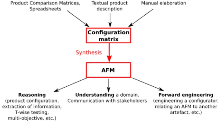
Figure 1: Core problem: synthesis of attributed fea-ture model from configuration matrix

formula. In prior works [5], we develop techniques for tak-ing the so-called ontological semantics into account when synthesizing feature models. Our work shares the goal of interactively supporting users – this time in the context of synthesizing attributed feature models.

Considering a broader view, reverse engineering techniques have been proposed to extract FMs from various artefacts (e.g., product descriptions [3, 16, 18, 25], architectural infor-mation [1] or source code [24]). However, they do not sup-port the synthesis of attributes despite the presence of non Boolean data in some of these artefacts. In this paper, we do not consider such a broad view; we focus solely on the synthesis of attributed FMs.

In addition to synthesis techniques, there are numerous existing academic (or industrial) languages and tools for specifying and reasoning about FMs [4, 8, 11–13, 19]. None of the existing tools propose support for synthesizing at-tributed FMs.

3.

MOTIVATION AND BACKGROUND

In this section, we motivate the need for an automated encoding of product descriptions as attributed feature models (AFMs). We also introduce background related to AFMs.

3.1

Product Descriptions and Feature Models

Many modern companies provide solutions for customiza-tion and configuracustomiza-tion of their products to match the needs

of each specific customer. From a user’s perspective, it

means a large variety of products to choose from. It is there-fore crucial for companies not only to provide comprehensive descriptions of their products, but also to do it in an easily navigable manner.

Product descriptions are usually represented in tabular formats, such as spreadsheets and product comparison ma-trices. The objective of such formats is to describe the char-acteristics of a set of products in order to document and differentiate them. From now on, we will use the term con-figuration matrix to refer to these tabular formats. Con-figuration matrices provide an enumerative description of a set of products and are by definition not succinct. Feature models provide an alternative format with a compact and formalized view of a set of products.

Figure 1 summarizes our motivation for synthesizing an AFM from a configuration matrix. As shown in the upper part of Figure 1, the input to the synthesis algorithm is a

Id License License Language Lang WYSI Type Price Support uage WYG W1 Commercial 10 Yes Java Yes W2 NoLimit 20 No – Yes W3 NoLimit 10 No – Yes W4 GPL 0 Yes Python Yes

W5 GPL 0 Yes Perl Yes

W6 GPL 10 Yes Perl Yes

W7 GPL 0 Yes PHP No

W8 GPL 10 Yes PHP Yes

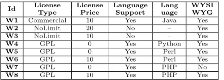
Figure 2: A configuration matrix for Wiki engines.

configuration matrix (see Definition 1).

Definition 1 (Configuration matrix). Let c1, ..., cM be a

given set of configurations. Each configuration ci is an N

-tuple (ci,1, ..., ci,N), where each element ci,j is the value of

a variable Vj. A variable represents either a feature or an

attribute. Using these configurations, we create an M × N

matrix C such that C = [c1, ..., cM]t, and call it a

configu-ration matrix.

Configuration matrices act as a formal, intermediate rep-resentation that can be obtained from various sources, such as (1) spreadsheets and product comparison matrices (e.g., see [7]), (2) disjunction of constraints, or (3) simply through a manual elaboration (e.g., practitioners explicitly enumer-ate and maintain a list of configurations [10]).

For instance, let us consider the domain of Wiki engines. The list of features supported by a set of Wiki engines can be documented using a configuration matrix. Figure 2 is a very simplified configuration matrix, which provides information about eight different Wiki engines.

The resulting AFM (see lower part of Figure 1) can as well be used to document a set of configurations and open new perspectives. First, state-of-the-art reasoning techniques for AFM can be reused (e.g., [4, 13, 19, 28]). Second, the hier-archy helps to structure the information and a potentially large number of features into multiple levels of increasing detail [14]; it helps to understand a domain or communi-cate with other stakeholders [8, 10, 14]. Finally, an AFM is central to many product line approaches and can serve as a basis for forward engineering [2] (e.g., through a mapping with source code or design models).

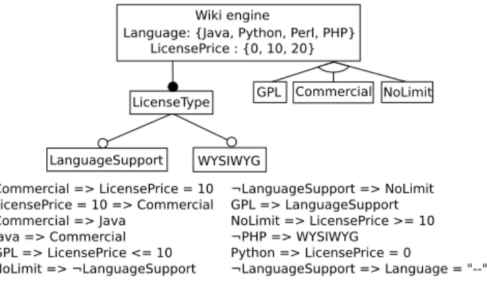
Overall, configuration matrices and feature models are se-mantically related and aim to characterize a set of config-urations. The two formalisms are complementary as they propose different views on the same product line; we aim to better understand the gap and switch from one repre-sentation to the other. For instance, Figure 3 depicts an at-tributed feature diagram as well as constraints that together provide one possible representation of the configuration ma-trix of Figure 2.

3.2

Attributed Feature Models

Several formalisms supporting attributes exist [4,9,12,17]. In this paper, we consider an extension of FODA-like FMs including attributes and inspired from the FAMA frame-work [8, 9]. An AFM is composed of an attributed feature diagram (see Definition 2 and Figure 4) and an arbitrary constraint (see Definition 3).

Definition 2 (Attributed Feature Diagram). An attributed

feature diagram (AFD) is a tuple hF , H, EM, GM T X, GXOR,

GOR, A, D, δ, α, RCi such that:

Commercial => LicensePrice = 10 LicensePrice = 10 => Commercial Commercial => Java Java => Commercial GPL => LicensePrice <= 10 NoLimit => ¬LanguageSupport ¬LanguageSupport => NoLimit GPL => LanguageSupport NoLimit => LicensePrice >= 10 ¬PHP => WYSIWYG Python => LicensePrice = 0 Wiki engine LanguageSupport LicenseType Language: {Java, Python,

Perl, PHP} LicensePrice: {0, 10, 20} GPL Commercial NoLimit

WYSIWYG

Φ = ¬WYSIWYG <=> PHP ∧ LicensePrice = 0

Figure 3: One possible attributed feature model for representing the configuration matrix in Figure 2

RC ::= bool factor ‘⇒’ bool factor

bool factor ::= feature name | ‘¬’ feature name | rel expr rel expr ::= attribute name rel op num literal rel op ::= ‘>’ | ‘<’ | ‘≥’ | ‘≤’ | ‘=’

Figure 4: The grammar of readable constraints.

• F is a finite set of boolean features.

• H = (F, E) is a rooted tree of features where E ⊆ F ×F is a set of directed child-parent edges.

• EM ⊆ E is a set of edges defining mandatory features.

• GM T X, GXOR, GOR ⊆ P (E\Em) are sets of feature

groups. The feature groups of GM T X, GXORand GOR

are non-overlapping and each feature group is a set of edges that share the same parent.

• A is a finite set of attributes.

• D is a set of possible domains for the attributes in A. • δ ∈ A → D is a total function that assigns a domain

to an attribute.

• α ∈ A → F is a total function that assigns an attribute to a feature.

• RC is a set of constraints over F and A that are con-sidered as human readable and may appear in the fea-ture diagram in a graphical or textual representation ( e.g., binary implication constraints can be represented as an arrow between two features).

A domain d ∈ D is a tuple hVd, 0d, <di with Vd a finite

set of values, 0d∈ Vd the null value of the domain and <d

a partial order on Vd. When a feature is not selected, all

its attributes bound by α take their null value, i.e., ∀(a, f ) ∈

α with δ(a) = hVa, 0a, <ai, we have ¬f ⇒ (a = 0a).

For the set of constraints in RC, formally defining what is human readable is essential for designing automated tech-niques that can synthesize RC. In this paper, we define RC

as the constraints that are consistent with the grammar2_in

Figure 4 (see bottom of Figure 3 for examples). We consider that these constraints are small enough and simple enough to be human readable. In this grammar, each constraint is a binary implication, which specifies a relation between the values of two attributes or features. Feature names and re-lational expressions over attributes are the boolean factors

2_{Other kinds of constraints (e.g., based on arithmetic}

op-erators) can be considered as well. They may be compu-tationally expensive to synthesize and require the use of constraint-based solvers.

that can appear in an implication. Further, we only allow natural numbers as numerical literals (num literal).

The grammar of Figure 4 and the formalism of attributed feature diagrams (see Definition 2) are not expressively com-plete regarding propositional logics, and therefore cannot represent any set of configurations (more details are given in Section 4.2). Therefore, to enable accurate representation of any possible configuration matrix, an AFM is composed of an AFD and a propositional formula:

Definition 3 (Attributed Feature Model). An attributed feature model is a pair hAF D, Φi where AFD is an attributed feature diagram and Φ is an arbitrary constraint over F and A that represents the constraints that cannot be expressed by RC.

Example. Figure 3 shows an example of an AFM describ-ing a product line of Wiki engines. The feature WikiMatrix is the root of the hierarchy. It is decomposed in 3 features: LicenseType which is mandatory and WYSIWYG and Lan-guageSupport which are optional. The xor-group composed of GPL, Commercial and NoLimit defines that the wiki en-gine has exactly 1 license and it must be selected among these 3 features. The attribute LicensePrice is attached to the feature LicenseType. The attribute’s domain states that it can take a value in the following set: {0, 10, 20}. The readable constraints and Φ for this AFM are listed below its hierarchy (see Figure 3). The first one restricts the price of the license to 10 when the feature Commercial is selected.

The main objective of an AFM is to define the valid con-figurations of a product line. A configuration of an AFM is defined as a set of selected features and a value for every attribute. A configuration is valid if it respects the con-straints defined by the AFM (e.g., the root feature of an AFM is always selected). The set of valid configurations corresponds to the configuration semantics of the AFM (see Definition 4).

Definition 4 (Configuration semantics). The configuration

semantics_{JmK of an AFM m is the set of valid configurations}

represented by m.

4.

SYNTHESIS FORMALIZATION

Two main challenges of synthesizing an AFM from a con-figuration matrix are (1) preserving the concon-figuration se-mantics of the input matrix; and (2) producing a maximal and readable diagram for a further exploitation by practi-tioners (see Figure 1). Synthesizing an AFM that represents the exact same set of configurations (i.e., configuration se-mantics) as the input configuration matrix is primordial; a too permissive AFM would expose the user to illegal config-urations. To prevent this situation, the algorithm must be sound (see Definition 5). Conversely, if the AFM is too con-strained, it would prevent the user from selecting available

configurations, resulting in unused variability. Therefore,

the algorithm must also be complete (see Definition 6). Definition 5 (Soundness of AFM Synthesis). A synthesis algorithm is sound if the resulting AFM (af m) represents only configurations that exist in the input configuration

ma-trix (cm), i.e.,_{Jaf mK ⊆ JcmK.}

Definition 6 (Completeness of AFM Synthesis). A synthe-sis algorithm is complete if the resulting AFM (af m) repre-sents at least all the configurations of the input configuration

matrix (cm), i.e.,_{JcmK ⊆ Jaf mK.}

To avoid the synthesis of a trivial AFM (e.g., an AFM with the input matrix encoded in the constraint Φ and no hierarchy, i.e., E = ∅), we target a maximal AFM as output (see Definition 7). Intuitively, we enforce that the feature diagram contains as much information as possible. Defini-tion 8 formulates the AFM synthesis problem.

Definition 7 (Maximal Attributed Feature Model). An AFM is maximal if its hierarchy H connects every feature in F and if none of the following operations are possible without modifying the configuration semantics of the AFM:

• add an edge to EM

• add a group to GM T X, GXORor GOR

• move a group from GM T X or GOR to GXOR

• add a constraint to RC that is not redundant with other constraints of RC or the constraints induced by the hierarchy and feature groups.

Definition 8 (Attributed Feature Model Synthesis Prob-lem). Given a set of configurations sc, the problem is to

synthesize an AFM m such that _{JscK = JmK ( i.e., the}

syn-thesis is sound and complete) and m is maximal.

4.1

Synthesis Parametrization

In Definition 8, we enforce the AFM to be maximal to avoid trivial solutions to the synthesis problem. Despite this restriction, the solution to the problem may not be unique. Given a set of configurations (i.e., a configuration matrix), multiple maximal AFMs can be synthesized.

This property has already been observed for the synthesis of Boolean FMs [5, 26, 27]. Extending boolean FMs with at-tributes exacerbates the situation. In some cases, the place of the attributes and the constraints over them can be modi-fied without affecting the configuration semantics of the syn-thesized AFM.

GPL Commercial NoLimit

WYSIWYG Wiki engine

Language: {Java, Python, Perl, PHP}

LanguageSupport LicensePrice : {0, 10, 20} LicenseType Commercial => LicensePrice = 10 LicensePrice = 10 => Commercial Commercial => Java Java => Commercial GPL => LicensePrice <= 10 NoLimit => ¬LanguageSupport ¬LanguageSupport => NoLimit GPL => LanguageSupport NoLimit => LicensePrice >= 10 ¬PHP => WYSIWYG Python => LicensePrice = 0 ¬LanguageSupport => Language = "--" Φ = ¬WYSIWYG <=> PHP ∧ LicensePrice = 0

Figure 5: Another attributed feature model repre-senting the configuration matrix in Figure 2

Example. Figures 3 and 5 depict two AFMs represent-ing the same configuration matrix of Figure 2. They have the same configuration semantics but their attributed fea-ture diagrams are different. In Figure 3, the feafea-ture WYSI-WYG is placed under Wiki engine whereas in Figure 5, it is placed under the feature LicenseType. Besides the attribute LicensePrice is placed in feature LicenseType in Figure 3, whereas it is placed in feature Wiki engine in Figure 5.

To synthesize a unique AFM, our algorithm uses domain knowledge, which is extra information that can come from

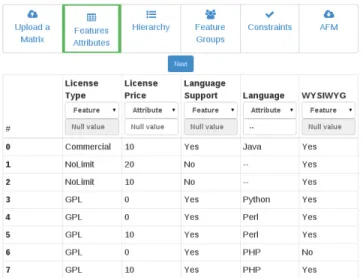
Figure 6: Web-based tool for gathering domain knowledge during the synthesis

heuristics, ontologies or a user of our algorithm. This do-main knowledge can be provided interactively during the synthesis or as input before the synthesis. Our synthesis tool (Figure 6 shows the workflow) provides an interface for collecting the domain knowledge so that users can:

• decide if a column of the configuration matrix should be represented as a feature or an attribute;

• give the interpretation of the cells (type of the data, partial order);

• select a possible hierarchy, including the placement of each attribute among their legal possible positions; • select a feature group among the overlapping ones; • provide specific bounds for each attribute in order to

compute meaningful and relevant constraints for RC. All steps are optional; in case the domain knowledge is missing, the synthesis algorithm (see next section) takes ar-bitrary yet sound decisions (e.g., random hierarchy).

Example. The domain knowledge that leads to the syn-thesis of the AFM of Figure 3 can be collected with our synthesis tool. Users specify what constitute an attribute or a feature. For instance, the column Language represents an attribute (for which the null value is ”–”). In further step, users can specify hierarchy and also precise that, e.g., ”10” is an interesting value for LicensePrice when synthesizing constraints.

4.2

Over-approximation of the Attributed

Fea-ture Diagram

A crucial property of the output AFM is to characterize the exact same configuration semantics as the input config-uration matrix (see Definition 8). In fact, the attributed feature diagram may over-approximate the configuration

se-mantics, i.e., _{JcmK ⊆ JF DK.} Therefore the additional

con-straint Φ of an AFM (see Definition 3) is required for pro-viding an accurate representation for any arbitrary configu-ration matrix.

Example. The diagrammatic part of the AFM in Figure 3 characterizes two additional configurations that are not in the matrix of Figure 2: {LicenseType = GPL, LicensePrice

= 0, LanguageSupport = Yes, Language = PHP, WYSI-WYG = Yes} and {LicenseType = GPL, LicensePrice = 10, LanguageSupport = Yes, Language = PHP, WYSIWYG = No}. To properly encode the configuration semantics of the configuration matrix, the AFM has to rely on a con-straint Φ. This particular concon-straint cannot be expressed by an attributed feature diagram as defined in Definition 2. Therefore, if Φ is not computed the AFM would represent an over-approximation of the configuration matrix.

A basic strategy for computing Φ is to directly encode the

configuration matrix as a constraint, i.e.,_{JcmK = JΦK. Such}

a constraint can be achieved using the following equation, where N is the number of columns and M is the number of rows. Φ = M _ i=1 N ^ j=1 (Vj= cij) (1)

An advantage of this approach is that the computation is immediate and Φ is, by construction, sound and complete w.r.t. the configuration semantics. The disadvantage is that some constraints in Φ are likely to be (1) redundant with the attributed feature diagram; (2) difficult to read and under-stand for a human.

Ideally, Φ should express the exact and sufficient set of constraints not expressed in the attributed feature diagram,

i.e., _JΦK = _{JcmK \ JF DK.} Synthesizing a minimal set of

constraint may require complex and time-consuming com-putations. The development of efficient techniques for sim-plifying Φ and investigating the usefulness and readability

of arbitrary constraints3 _{are out of the scope of this paper.}

5.

SYNTHESIS ALGORITHM

Algorithm 1 presents a high-level description of our ap-proach for synthesizing an Attributed Feature Diagram (AFD). The two inputs of the algorithm are a configuration matrix and some domain knowledge for parametrizing the synthesis. The output is a maximal AFD. In complement to the AFD, we compute the constraint Φ (as described by Equation 1). The addition of Φ and the AFD forms the AFM.

5.1

Extracting Features and Attributes

The first step of the synthesis algorithm is to extract the features (F ), the attributes (A) and their domains (D, δ). This step essentially relies on the domain knowledge to de-cide how each column of the matrix must be represented as a feature or an attribute. We also discard all the dead features, i.e., features that are always absent. The domain knowledge specifies which values in the corresponding col-umn indicate the presence (e.g., by default ”Yes”) or absence (e.g., ”No”) of the feature. For each attribute, all the dis-tinct values of its corresponding column form the first part

of its domain (Vd). The other parts, the null value 0d, and

the partial order <d, are computed accordingly. Some

pre-defined heuristics are implemented to populate the domain knowledge and consist in (1) determining whether a column is a feature or an attribute or (2) typing the domain values. If needs be, users can override the default behaviour of the synthesis and specify domain knowledge.

3

We recall that relational constraints as defined by the grammar of Figure 4 are already part of the synthesis. Arbi-trary constraints represent other forms of constraints involv-ing more than two features or attributes – hence questioninvolv-ing their usefulness or readability by humans.

Algorithm 1Attributed Feature Diagram Synthesis Require: A configuration matrix MTX and domain knowledge

DK

Ensure: An attributed feature diagram AFD

Extract the features, the attributes and their domains 1 (F, A, D, δ) ← extractFeaturesAndAttributes(M T X, DK)

Compute binary implications

2 BI ← computeBinaryImplications(M T X) Define the hierarchy

3 (BIG, M T XG) ← computeBIGAndMutexGraph(F, BI) 4 H ← extractHierarchy(BIG, DK)

5 α ← placeAttributes(BI, F, A, DK) Compute the variability information 6 EM ← computeMandatoryFeatures(H, BIG)

7 F G ← computeFeatureGroups(H, BIG, M T XG, DK) Compute cross tree constraints

8 RC ← computeConstraints(BI, DK, H, EM, F G)

Create the attributed feature diagram

9 return AF D(F , H, EM, F G, A, D, δ, α, RC)

Example. Let us consider the variable LanguageSupport

in the configuration matrix of Figure 2. Its domain has

only 2 possible Boolean values: Yes and No. Therefore, the variable LanguageSupport is identified as a feature. Follow-ing the same process, WYSIWYG and LicenseType are also identified as features while the other variables are identified as attributes. For instance, LicensePrice is an attribute and its domain is the set of all values that appear in its column: {0, 10, 20}.

5.2

Extracting Binary Implications

An important step of the synthesis is to extract binary implications between features and attributes. A binary im-plication, for a given configuration matrix C, is of the form

(vi= u) ⇒ (vj∈ Si,j,u), where i and j indicate two distinct

columns of C, and Si,j,uis the set of all values in the jth

col-umn of C, for which the corresponding cell in the ith colcol-umn is equal to u. We denote the set of all binary implications of C as BI(C). Algorithm 2 computes this set. The algorithm iterates over all pairs (i, j) of columns and all configurations

ckin C to compute S(i, j, ck,i) (i.e., Si,j,ck,i).

Algorithm 2computeBinaryImplications

Require: A configuration matrix C Ensure: A set of binary implications BI

1 BI ← ∅

2 for all (i, j) such that 1 ≤ i, j ≤ N and i 6= j do 3 for all cksuch that 1 ≤ k ≤ M do

4 if S(i, j, ck,i) does not exists then

5 S(i, j, ck,i) ← {ck,j}

6 BI ← BI ∪ {hi, j, u, S(i, j, ck,i)i}

7 else

8 S(i, j, ck,i) ← S(i, j, ck,i) ∪ {ck,j}

9 return BI

In line 4, the algorithm tests if S(i, j, ck,i) already exists.

If so, the algorithm simply adds ck,j, the value of column

j for configuration ck, to the set S(i, j, ck,i). Otherwise,

S(i, j, ck,i) is initialized with a set containing ck,j. Then,

a new binary implication is created and added to the set BI. At the end of the inner loop, BI contains all the binary

implications of all pairs of columns (i, j).

5.3

Defining the Hierarchy

The hierarchy H of an AFD is a rooted tree of features

such that ∀(f1, f2) ∈ E, f1⇒ f2, i.e., each feature implies its

parent. As a result, the candidate hierarchies, whose parent-child relationships violate this property, can be eliminated upfront. To guide the selection of a legal hierarchy for the AFD, we rely on the Binary Implication Graph (BIG) of a configuration matrix:

Definition 9 (Binary Implication Graph (BIG)). A binary implication graph of a configuration matrix C is a directed

graph (VBIG, EBIG) where VBIG= F and EBIG= {(fi, fj) |

(fi⇒ fj) ∈ BI(C)}.

The BIG aims to represent all the binary implications, thus representing every possible parent-child relationships in a legal hierarchy. We compute the BIG as follows: for each constraint in BI (see Algorithm 2) involving two features we add an edge in the BIG. Hierarchy H of the AFD is a rooted tree inside the BIG. In general, it is possible to find many such trees. As part of the tool (see Figure 6), users can spec-ify domain knowledge to select a tree. The BIG is exploited to interactively assist users in the selection of the AFD’s hierarchy. In case the domain knowledge is incomplete, a branching of the graph (the counterpart of a spanning tree for undirected graphs) is randomly computed [5].

After choosing the hierarchy of features, we focus on the placement of attributes. An attribute a can be placed in a

feature f if ¬f ⇒ (a = 0a). As a result, the candidate

fea-tures verifying this property are considered as legal positions

for the attribute. We promote, according to the domain

knowledge, one of the legal positions of each attribute.

Example. In Figure 2, the attribute Language has a

domain d with “–” as its null value, i.e., 0d= “–”. This null

value restricts the place of the attribute. The property ¬f ⇒

(a = 0a) of Definition 2 holds for the attribute Language and

the feature LanguageSupport. However, the configuration W7 forbids the attribute to be placed in feature WYSIWYG. The value of Language is not equal to its null value when WYSIWYG is not selected.

5.4

Computing the Variability Information

As the hierarchy of an AFD is made of features only, attributes do not impact the computation of the variabil-ity information (optional/mandatory features and feature groups). Therefore, we can rely on algorithms that have been developed for Boolean FMs [5, 26, 27].

First, for the computation of mandatory features, we rely on the BIG as it represents every possible implication be-tween two features. For each edge (c, p) in the hierarchy, we check that the inverted edge (p, c) exists in the BIG. In

that case, we add this edge to EM.

For feature groups, we reuse algorithms from the synthesis of Boolean FMs [5,26,27]. For the sake of self-containedness, we briefly describe the computation of each type of group.

For mutex-groups (GM T X), we compute a so-called mutex

graph that contains an edge whenever two features are mu-tually exclusive. The maximum cliques of this mutex graph are the mutex-groups [26, 27].

For or-groups (GOR), we translate the input matrix to a

binary integer programming problem [27]. Finding all solu-tions to this problem results in the list of or-groups.

For xor-groups (GXOR), we consider mutex-groups since

a xor-group is a mutex-group with an additional constraint stating that at least one feature of the group should be

se-lected. We check, for each mutex-group, that its parent

implies the disjunction of the features of the group. For

that, we iterate over the binary implications (BI) until we find that the property is inconsistent. To ensure the max-imality of the resulting AFM, we discard any or-group or mutex-group that is also an xor-group.

Finally, the features that are not involved in a mandatory relation or a feature group are considered optional.

5.5

Computing Cross Tree Constraints

The final step of the AFD synthesis algorithm is to com-pute cross tree constraints (RC). We generate three kinds of constraints: requires, excludes and relational constraints. A requires constraint represents an implication between two features. All the implications contained in the BIG (i.e., edges) that are not represented in the hierarchy or manda-tory features, are promoted as requires constraints (e.g., the implication Commercial ⇒ Java in Figure 3).

Excludes constraints represent the mutual exclusion of

two features. Such constraints are contained in the

mu-tex graph. As the previously computed mumu-tex-groups may not represent all the edges of the mutex graph, we pro-mote the remaining edges of the mutex graph as excludes constraints. For example, the features NoLimit and Lan-guageSupport, in Figure 3, are mutually exclusive. This re-lation is included in RC as an excludes constraint: NoLimit ⇒ ¬LanguageSupport.

Finally, relational constraints are all the constraints fol-lowing the grammar described in Figure 4 and involving at least one attribute. Admittedly there is a huge number of possible constraints that respect the grammar of RC. Our algorithm relies on some domain knowledge (see Figure 6) to restrict the domain values of attributes considered for the computation of RC. Formally, the knowledge provides the information required for merging binary implications as

(ai, k) pairs, where aiis an attribute, and k belongs to Di.

In case the knowledge is incomplete (e.g., users do not spec-ify a bound for an attribute), we randomly choose a value among the domain of an attribute.

Then the algorithm proceeds as follows. First, we trans-form each constraint referring to one feature and one at-tribute to a constraint that respects the grammar of RC. Then, we focus on constraints in BI that involve two at-tributes and we merge them according to the domain

knowl-edge. Using the pairs (ai, k) of the domain knowledge, we

partition the set of all binary implications with ai = u on

the left hand side of the implication into three categories: those with u < k, those with u = k, and those with u > k.

Let bj,1, ..., bj,pbe all such binary implications, belonging to

the same category, and involving aj(i.e., each bj,r is of the

form (ai= ur⇒ aj∈ Sr)). We merge these binary

implica-tions into a single one: (ai∈ {u1, ..., up} ⇒ aj∈ S1∪...∪Sp)

whenever the conformance of the grammar of RC holds.

Example. From the configuration matrix of Figure 2,

we can extract the following binary implication: GPL ⇒ LicensePrice ∈ {0, 10}. We also note that the domain of LicensePrice is {0, 10, 20}. Therefore, the right side of the binary implication can be rewriten as LicensePrice <= 10. As this constraint can be expressed by the grammar of RC, we add GPL ⇒ LicensePrice <= 10 to RC (see Figure 3).

6.

EVALUATION ON RANDOM MATRICES

We developed a tool4 that implements Algorithm 1. The

tool is mainly implemented in Scala programming language. Algorihtm 2 is written in pure Scala and relies on appro-priate data structures (e.g., HashMap and HashSet) for ef-ficient computation of implications. For the computation of

or-groups, we rely on the SAT4J solver5_.

To provide an insight into the scalability of our proce-dure, we experimentally evaluate the runtime complexity of our AFD synthesis procedure. For this purpose, we have developed a random matrix generator, which takes as input three parameters:

• number of variables (features and attributes) • number of configurations

• maximum domain size (i.e., maximum number of dis-tinct values in a column)

The type of each variable (feature or attribute) is ran-domly selected according to a uniform distribution. An im-portant property is that our generator does not ensure that the number of configurations and the maximum domain size are reached at the end of the generation. Any duplicated configuration or missing value of a domain is not corrected. Therefore, the parameters entered for our experiments may not reflect the real properties of the generated matrices. To avoid any misinterpretation or bias, we present the concrete numbers in the following results.

Moreover, to reduce fluctuations caused by the random generator, we perform the experiments at least 100 times for each triplet of parameters. In order to get the results in a reasonable time, we used a cluster of computers. Each node in the cluster is composed of two Intel Xeon X5570 at 2.93 Ghz with 24GB of RAM.

6.1

Initial Experiments with Or-groups

We first perform some initial experiments on random ma-trices. We quickly notice that computation of the or-groups posed a scalability problem. It is not surprising since this part of the synthesis algorithm is NP-hard, leading to some timeouts even for Boolean FMs (e.g., see [27]).

Specifically, we measured the time needed to compute the or-groups from a matrix with 1000 configurations, a maxi-mum domain size of 10 and a number of variables ranging from 5 to 70. To keep a reasonable time for the execution of the experiment, we set a timeout at 30 minutes. Results are presented in Figure 7. The red dots indicate average values in each case. The results confirm that the computa-tion of or-groups quickly becomes time consuming. The 30 minutes timeout is reached with matrices containing only 30 variables. With at least 60 variables, the timeout is system-atically reached. Therefore, we deactivated the computation of or-groups in the following experiments.

6.2

Scalability w.r.t the number of variables

To evaluate the scalability with respect to the number of variables, we perform the synthesis of random matrices with 1000 configurations, a maximum domain size of 10 and a number of variables ranging from 5 to 2000. In Figure 8, we present the square root of the time needed for the whole

4

The complete source code can be found in https://github. com/gbecan/FOReverSE-AFMSynthesis

5

Time (min) Number of variables 1 5 10 15 20 25 30 5 10 15 20 25 30 35 40 50 60 70 Time (min) Number of variables 1 5 10 15 20 25 30 5 10 15 20 25 30 35 40 50 60 70

Figure 7: Scalability of or-groups computation w.r.t the number of variables

Squar e r oot of time (s (1/2) ) Number of variables 0 10 20 30 40 5 100 200 500 _{1000 2000}

Figure 8: Scalability w.r.t the number of variables

synthesis compared to the number of variables. As shown by the linear regression line, the square root of the time grows linearly with the number of variables, with a correlation co-efficient of 0.997.

6.3

Scalability w.r.t the number of

configura-tions

To evaluate the scalability with respect to the number of configurations, we perform the synthesis of random matrices with 100 variables, a maximum domain size of 10 and a number of configurations ranging from 5 to 200,000. With 100 variables, and 10 as the maximum domain size, we can

generate 10100 _{distinct configurations. This number is big}

800 600 400 200 0 Time (s) Number of configurations

1e+03 1e+04 2e+04 5e+04 1e+05 2e+05

Figure 9: Scalability w.r.t the number of configura-tions Squar e r oot of time (s (1/2) )

Maximum domain size

0 10 20 30 40 50 60 5 200 500 _{1000 2000 5000}

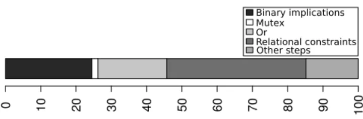
Figure 10: Scalability w.r.t the maximum domain size 0 _{10 20 30 40 50 60 70 80 90} 100 Binary implications Mutex Relational constraints Other steps

Figure 11: Time complexity distribution for all ex-periments without or-groups computation

enough to ensure that our generator can randomly generate 5 to 200,000 distinct configurations.

Figure 9 reports the synthesis time in each case. As shown in this figure, the time grows linearly with the number of configurations, and the correlation coefficient is 0.997.

6.4

Scalability w.r.t the maximum domain size

To evaluate the scalability with respect to the maximum domain size, we perform the synthesis of random matrices with 10 variables, 10,000 configurations and a maximum

do-main size ranging from 5 to 10,0006.

Figure 10 presents the square root of the synthesis time. We notice that for each value of the domain size, the points are distributed in small groups. For instance, we can see nine groups of points for a maximum domain size of 2000. Each group represents the execution of our algorithm with matrices that have the same number of attributes. However, we see that the number of attributes does not significantly affect the maximum domain size (the maximum domain size is approximately the same for all groups of results).

A linear regression line fits the average square root of the time, with a correlation coefficient of 0.932. This implies that the synthesis time grows quadratically with the maxi-mum domain size.

6.5

Time Complexity Distribution

To further understand the overall time complexity, we an-alyze its distribution over different steps of the algorithm (see Figure 11). The results clearly show that the major part of the algorithm is spent on the computation of binary implications and relational constraints for RC. The rest of

6_{Our random matrix generator cannot ensure that the}

max-imum domain sizes are always reached. It explains why we report in Figure 10 the measures for a maximum domain size of 4,385 (resp. 6,416) instead of 5000 (resp. 10,000).

Table 1: Statistics on the Best Buy dataset.

Min Median Mean Max Variables 23 50.0 48.6 91 Configurations 11 27.0 47.1 203 Max domain size 11 27.0 47.1 203 Empty cells before interpretation 2.5% 16.1% 14.4% 25.0%

the synthesis represents less than 10% of the total duration. According to our theoretical analysis (see [6] for details), the two hard parts of the synthesis algorithm are the com-putation of mutex-groups (exponential complexity) and or-groups (NP-complete). We note that 93.8% of the configura-tion matrices in our dataset produce mutex graphs that con-tain absolutely no edges. In such cases, computing mutex-groups is trivial. The rest of the algorithm has a polynomial complexity, which is confirmed by the experiments presented in this section.

7.

EVALUATION ON REAL MATRICES

To provide an insight into the scalability of our approach on realistic configuration matrices, we executed our algo-rithm on configuration matrices extracted from Best Buy website. Best Buy is a well known American company that sells consumer electronics. On their website, the description of each product is completed with a matrix that describes technical information. Each matrix is formed of two columns in order to associate a feature or an attribute of a product to its value. The website offers a way to compare products that consists in merging the matrices to form a single con-figuration matrix which is similar to the one in Figure 2.

7.1

Experimental Settings

We developed an automated technique to extract

config-uration matrices from Best Buy website. The procedure

is composed of 3 steps. First, it selects a set of products whose matrices have at least 75% of feature and attributes in common. Then, it merges the corresponding matrices of the selected product to obtain a configuration matrix. Un-fortunately, the resulting configuration matrix may contain empty cells. Such cells have no clear semantics from a vari-ability point of view. The last step of the procedure consists in giving an interpretation to these cells. If a feature or an attribute contain only integers, the empty cells are inter-preted as ”0”. Otherwise, the empty cells are interinter-preted as ”No” which means that the feature or attribute is absent.

With this procedure, we extracted 242 configuration ma-trices from the website that form our dataset for the exper-iment. Table 1 reports statistics on the dataset about the number of variables, configurations, the maximum domain size and the number of empty cells before interpretation.

In the following experiments, we measure the execution time of Algorithm 1 on the Best Buy dataset. We execute the algorithm on the same cluster of computers in order to have comparable results with previous experiments on ran-dom matrices. We also execute the synthesis 100 times for each configuration matrix of the dataset in order to reduce fluctuations caused by other programs running on the clus-ter and the random decisions taken during the synthesis.

7.2

Scalability

We first measure the execution time of Algorithm 1 with the computation of or-groups activated. On the Best Buy

0 _{10 20 30 40 50 60 70 80 90 100} Binary implications Mutex Relational constraints Other steps Or

Figure 12: Time complexity distribution of Algo-rithm 1 on the Best Buy dataset

dataset, the execution time of Algorithm 1 is 0.8s in average with a median of 0.5s. The most challenging configuration matrix has 73 variables, 203 configurations and a maximum domain size of 203. The synthesis of an AFM from this ma-trix takes at most 274.7s. Figure 12 reports the average dis-tribution for the dataset. It shows that the computation of binary implications, or-groups and the relational constraints are the most time-consuming tasks. It confirms the results of the experiments on random matrices. However, we note that on the Best Buy dataset, the computation of or-groups can be executed in a reasonable time.

To further compare with previous experiments, we per-formed the same experiment but with the computation of or-groups deactivated. In these conditions, the execution time of Algorithm 1 is 0.5s in average with a median of 0.4s. This time, the most challenging configuration matrix has 77 variables, 185 configurations and a maximum domain size of 185. The synthesis of its corresponding AFM takes only 2.1s. The experiments confirm that the computation of or-groups is the hardest part of the algorithm. It also shows that the synthesis algorithm ends in reasonable time for all the configuration matrices of the Best Buy dataset.

Moreover, the execution time on a random matrix with 100 variables, 200 configurations and a maximum domain size of 10 is at most 2.3s. It indicates that the execution time on the most challenging matrix of the Best Buy dataset has the same order of magnitude as the execution time on a similar random matrix.

8.

THREATS TO VALIDITY

An external threat is that the evaluation of Section 6 is based on the generation of random matrices. Using such matrices may not reflect the practical complexity of our

al-gorithm. To mitigate this threat we complement with a

realistic data set (Best Buy).

Evaluating the scalability on a cluster of computers in-stead of a single one may impact the scalability results and is an internal threat to validity. We use a cluster composed of identical nodes to limit this threat. Even if the nodes do not represent standard computers, the practical complexity of the algorithm is not influenced by this gain of processing power. Moreover, all the necessary data for the experiments are present in the local disks of the nodes thus avoiding any network related issue. Finally, we performed 100 runs for each set of parameters in order to reduce any variation of performance. Another threat to internal validity is related to our interpretation of cell values in realistic matrices of Section 7. Another semantics for empty cells may have an influence on the results. Our initial experiments (not re-ported in this paper) did not reveal significant changes.

manually reviewed some resulting AFMs. We also tested the algorithm against a set of manually designed configuration matrices. Each matrix represents a minimal example of a construct of an AFM (e.g., one of the matrices represents an AFM composed of a single xor-group). The test suite covers all the concepts in an AFM. None of these experi-ments revealed any anomalies in our implementation.

9.

CONCLUSION

In this paper, we presented the foundations for synthesiz-ing attributed feature models (AFMs) from product descrip-tions. We introduced the formalism of configuration matrix for documenting a set of products along different Boolean and numerical values. The key contributions of the paper can be summarized as follows:

• We described formal properties of AFMs (over-approximation, equivalence) and established semantic correspondences with the formalism of configuration matrices (Section 4);

• We designed and implemented a tool-supported, para-meterizable synthesis algorithm (Section 5);

• We empirically evaluated the scalability of the syn-thesis algorithm on random (Section 6) and real-world matrices (Section 7).

A first research direction is to investigate how approaches for mining variability and constraints can fed our synthesis algorithm – this time with the support of attributes.

As part of our experiments, we report that the number of constraints synthesized for the random dataset is 237 in average with a maximum of 8906. The Best Buy dataset ex-hibits 6281 constraints in average with a maximum of 28300 (we can assume there are more constraints since the number of configuration is lower). Hence our work identifies a new important research direction: how to deal with the huge amount of constraints that can be synthesized? It seems not reasonable to present all constraints to a human. Hence the challenge is to synthesize or present only a readable and useful portion of constraints. Numerous strategies can be considered, e.g., minimisation [29], prioritization, or letting users control the constraints they want.

Acknowledgements. Experiments presented in this pa-per were carried out using the Grid’5000 (see https://www. grid5000.fr).

10.

REFERENCES

[1] M. Acher, A. Cleve, P. Collet, P. Merle, L. Duchien, and P. Lahire. Extraction and evolution of architectural variability models in plugin-based systems. SoSyM, 2013. [2] S. Apel, D. Batory, C. K¨astner, and G. Saake.

Feature-Oriented Software Product Lines: Concepts and Implementation. Springer-Verlag, 2013.

[3] E. Bagheri, F. Ensan, and D. Gasevic. Decision support for the software product line domain engineering lifecycle. Automated Software Engineering, 19(3):335–377, 2012. [4] K. Bak, K. Czarnecki, and A. Wasowski. Feature and

meta-models in clafer: mixed, specialized, and coupled. In SLE’10, 2011.

[5] G. B´ecan, M. Acher, B. Baudry, and S. Ben Nasr. Breathing ontological knowledge into feature model synthesis: an empirical study. Empirical Software Engineering, 2015.

[6] G. B´ecan, R. Behjati, A. Gotlieb, and M. Acher. Synthesis of attributed feature models from product descriptions: Foundations. arXiv preprint arXiv:1502.04645, 2015.

[7] G. B´ecan, N. Sannier, M. Acher, O. Barais, A. Blouin, and B. Baudry. Automating the formalization of product comparison matrices. In ASE, 2014.

[8] D. Benavides, S. Segura, and A. Ruiz-Cortes. Automated analysis of feature models 20 years later: a literature review. Information Systems, 35(6), 2010.

[9] D. Benavides, S. Segura, P. Trinidad, and A. R. Cort´es. Fama: Tooling a framework for the automated analysis of feature models. VaMoS, 2007.

[10] T. Berger, D. Nair, R. Rublack, J. M. Atlee, K. Czarnecki, and A. Wasowski. Three cases of feature-based variability modeling in industry. In MODELS, 2014.

[11] T. Berger, R. Rublack, D. Nair, J. M. Atlee, M. Becker, K. Czarnecki, and A. Wasowski. A survey of variability modeling in industrial practice. In VaMoS’13, 2013. [12] A. Classen, Q. Boucher, and P. Heymans. A text-based

approach to feature modelling: Syntax and semantics of TVL. Sci. Comput. Program., 76(12), 2011.

[13] M. Cordy, P.-Y. Schobbens, P. Heymans, and A. Legay. Beyond boolean product-line model checking: dealing with feature attributes and multi-features. In ICSE, 2013. [14] K. Czarnecki, C. H. P. Kim, and K. T. Kalleberg. Feature

models are views on ontologies. In SPLC, 2006.

[15] K. Czarnecki, S. She, and A. Wasowski. Sample spaces and feature models: There and back again. In SPLC, 2008. [16] J.-M. Davril, E. Delfosse, N. Hariri, M. Acher,

J. Cleland-Huang, and P. Heymans. Feature model extraction from large collections of informal product descriptions. In ESEC/FSE, 2013.

[17] H. Eichelberger and K. Schmid. Mapping the design-space of textual variability modeling languages: a refined analysis. STTT, pages 1–26, 2014.

[18] A. Ferrari, G. O. Spagnolo, and F. dell’Orletta. Mining commonalities and variabilities from natural language documents. In SPLC, 2013.

[19] J. Guo, E. Zulkoski, R. Olaechea, D. Rayside, K. Czarnecki, S. Apel, and J. M. Atlee. Scaling exact multi-objective combinatorial optimization by parallelization. In ASE, 2014.

[20] E. N. Haslinger, R. E. Lopez-Herrejon, and A. Egyed. On extracting feature models from sets of valid feature combinations. In FASE, 2013.

[21] A. Hubaux, T. T. Tun, and P. Heymans. Separation of concerns in feature diagram languages: A systematic survey. ACM Computing Surveys, 2013.

[22] M. Janota, V. Kuzina, and A. Wasowski. Model construction with external constraints: An interactive journey from semantics to syntax. In MODELS, 2008. [23] R. E. Lopez-Herrejon, L. Linsbauer, J. A. Galindo, J. A.

Parejo, D. Benavides, S. Segura, and A. Egyed. An assessment of search-based techniques for reverse engineering feature models. Journal of Systems and Software, 2014.

[24] S. Nadi, T. Berger, C. K¨astner, and K. Czarnecki. Mining configuration constraints: Static analyses and empirical results. In ICSE, 2014.

[25] U. Ryssel, J. Ploennigs, and K. Kabitzsch. Extraction of feature models from formal contexts. In FOSD, 2011. [26] S. She, R. Lotufo, T. Berger, A. Wasowski, and

K. Czarnecki. Reverse engineering feature models. In ICSE, 2011.

[27] S. She, U. Ryssel, N. Andersen, A. Wasowski, and K. Czarnecki. Efficient synthesis of feature models. Information and Software Technology, 56(9), 2014. [28] T. Th¨um, S. Apel, C. K¨astner, I. Schaefer, and G. Saake. A

classification and survey of analysis strategies for software product lines. ACM Computing Surveys, 2014.

[29] A. von Rhein, A. Grebhahn, S. Apel, N. Siegmund, D. Beyer, and T. Berger. Presence-condition simplification in highly configurable systems. In ICSE, 2015.