Reliable computation for geometric models

Direction des bibliothèques

AVIS

Ce document a été numérisé par la Division de la gestion des documents et des archives de l’Université de Montréal.

L’auteur a autorisé l’Université de Montréal à reproduire et diffuser, en totalité ou en partie, par quelque moyen que ce soit et sur quelque support que ce soit, et exclusivement à des fins non lucratives d’enseignement et de recherche, des copies de ce mémoire ou de cette thèse.

L’auteur et les coauteurs le cas échéant conservent la propriété du droit d’auteur et des droits moraux qui protègent ce document. Ni la thèse ou le mémoire, ni des extraits substantiels de ce document, ne doivent être imprimés ou autrement reproduits sans l’autorisation de l’auteur.

Afin de se conformer à la Loi canadienne sur la protection des renseignements personnels, quelques formulaires secondaires, coordonnées ou signatures intégrées au texte ont pu être enlevés de ce document. Bien que cela ait pu affecter la pagination, il n’y a aucun contenu manquant.

NOTICE

This document was digitized by the Records Management & Archives Division of Université de Montréal.

The author of this thesis or dissertation has granted a nonexclusive license allowing Université de Montréal to reproduce and publish the document, in part or in whole, and in any format, solely for noncommercial educational and research purposes.

The author and co-authors if applicable retain copyright ownership and moral rights in this document. Neither the whole thesis or dissertation, nor substantial extracts from it, may be printed or otherwise reproduced without the author’s permission.

In compliance with the Canadian Privacy Act some supporting forms, contact information or signatures may have been removed from the document. While this may affect the document page count, it does not represent any loss of content from the document.

Université de Montréal

Reliable Computation for Geometrie Models

par

Di Jiang

Département d'informatique et de recherche opérationnelle

Faculté des arts et des sciences

Thèse présentée

la Faculté des études supérieures et postdoctorales

en vue de l'obtention du grade de Philosophire Doctor (Ph.D.)

en informatique

Août 2008

©

Di Jiang, 2008

Université de Montréal

Faculté des études supérieures et postdoctorales

Cette thèse intitulée :

Reliable Computation for Geometrie Models

présentée par :

Di Jiang

a été évaluée par un jury composé des personnes suivantes:

Victor Ostromoukhov

Neil Stewart

Pierre Poulin

Wolfram Luther

Abraham Broer

Résumé

La modélisation géométrique est devenue un domaine de recherche et de développement central à un vaste champ d'applications. Avec la forte croissance de la puissance de calcul des ordinateurs, la simulation par ordinateur a commencé à jouer un rôle important dans plusieurs domaines de recherche reliés à la modélisation géométrique, de l'ingénierie traditionnelle à la simulation de chirurgie virtuelle.

À cause de l'usage de représentations de précision finie, l'absence de robustesse numérique en calcul scientifique est un phénomène bien connu et répandu. De nombreuses approches différentes ont été proposées pour résoudre ce problème. Les nombres en virgule flottante (IEEE 754/854) [PH98, OveOl] sont les substituts standards pour les nombres réels en calculs infor-matisés, et la plupart des logiciels de modélisation de solides, incluant les systèmes de concep-tion assistée par ordinateur (CAO), sont basés sur des méthodes de modélisaconcep-tion géométrique qui fonctionnent en utilisant l'arithmétique en virgule flottante. Mais cette dernière, appliquée naïvement, peut causer l'échec d'axiomes géométriques. L'analyse inverse d'erreur (backward error analysis), maintenant standard, est un outil très utile qui peut nous aider à surmonter ce

problème: elle nous permet de distinguer les algorithmes qui, en presence d'incertitudes dans les données, ont produit des résultats aussi bien que nous pouvions espérer.

L'impact de l'absence de robustesse daris le domaine de la modélisation géométrique a été ouvertement reconnu et il y a eu beaucoup d'attention pour améliorer la fiabilité. D'un autre côté, il existe plusieurs 'représentations en modélisation géométrique et, même si chacune par-vient à bien modéliser certaines propriétés, aucune d'elles n'est suffisamment générale pour sa-tisfaire tous les prérequis qui pourraient être souhaitables d'une représentation. Ainsi, pour des problèmes géométriques différents, l'absence de robustesse tend à se manifester de différentes façons et nous devons chercher la méthode appropriée pour chaque problème : une solution universelle n'existe pas.

iv

Le but de cette thèse est d'étudier le calcul informatisé fiable en modélisation géométrique. En particulier, nous abordons trois problèmes reliés à la robustesse en modélisation géométrique:

1. L'arithmétique en virgule flottante pour des problèmes de géométrie informatique avec des données incertaines (Floating-point arithmetic for computational-geometry problems

with uncertain data).

Dans ce travail, trois exemples (résolution de systèmes d'équations linéaires, le problème de l'enveloppe convexe planaire et un problème d'objet extrudé en trois dimensions) sont présentés pour expliquer notre méthode pour accomplir l'analyse inverse d'erreur. Aussi, notre exposition illustre le fait que l'analyse inverse d'erreur ne prétend pas surmonter le problème de précision finie, et que des situations en géométrie informatique sont exacte-ment parallèles à d'autres domaines informatiques.

2. Jonction fiable de surfaces pour des modèles combinant maillages et surfaces paramétriques

(Reliable joining of surfaces for combined mesh-surface models).

L'opérateur de jonction est un important opérateur primitif pour les opérations booléennes. Notre motivation pour ce travail est de chercher un algorithme de jonction fiable pour les patches combinant maillages et surfaces paramétriques, prenant en considération un

critère d'erreur sur la normale. Deux mesures d'erreur sont définies pour guider la procédure de jonction. En utilisant le théorème de l'extension de Whitney, la qualité de la jonction calculée peut être garantie.

3. Robustesse d'opérations booléennes sur les modèles de surface de subdivision (Robustness

of boolean operations on subdivision-surface models.)

Les surfaces de subdivision sont de plus en plus fréquemment utilisées comme représentation de rechange, à la place des surfaces B-splines rationnelles non uniformes coupées (trim-med NURBS), pour la modélisation géométrique dû à leurs avantages intrinsèques. En

particulier, elles permettent d'éviter le problème difficile de faire correspondre les bor-dures des patches coupées. Ce travail décrit un algorithme pour effectuer des opérations

booléennes, basé sur l'usage des maillages limites, dans le cas où les objets en entrée sont définis en termes de maillages triangulaires et de subdivision de Loop. Ce travail se concentre sur la robustesse, incluant des bornes d'erreurs et des méthodes numériques pour la validation a posteriori de la forme topolo~ique.

Mots-clés:

v

d'erreur, maillage de surfaces. jonction, opération booléenne, modèles d'interrogation de forme, erreur de vecteurs normaux, surfaces de subdivision.

Abstract

Geometric modeling has become a central area of research and development that involves di-verse applications. In fact, because of greatly increased computer power, computer simulation has started playing an important role in many geometric-modeling related research domains, from tradition al engineering design to virtual surgery simulation.

Due to the use of finite-precision representation, numerical nonrobustness in scientific com-puting is a well-known and widespread phenomenon. Several different approaches have been proposed for this problem. Floating-point numbers (IEEE 754/854) [PH98, OveOl] are the standard substitute for real numbers in computations, and most solid modelers, inc1uding CAD (Computer Aided Design) systems, are based on geometric-modeling methods that operate us-ing floatus-ing-point arithmetic. But naively applied floatus-ing-point arithmetic can cause axioms of geometry to fail. The now-standard backward error analysis is a very useful tool that can help to overcome this problem: it permits us to distinguish those algorithms which, given the presence of uncertainties in the data, have done as weIl as we can hope for.

The impact of nonrobustness in the domain of geometric modeling has been widely ac-knowledged, and much attention has been paid to improving reliability. On the other hand, many different geometric modeling representations exist, and although each succeeds in mod-eling certain properties weIl, none of them is general enough to satisfy aIl the requirements that could be demanded of a representation. Therefore, for different geometric problems, nonro-bustness tends to manifest itself in different ways, and we must seek an appropriate method for each problem: a universal solution does not exist.

The goal of this thesis is to study reliable computation for geometric models. More specifi-caIly, we will address three related robustness problems in geometric modeling:

1. Floating-point arithmetic for computational-geometry problems with uncertain data. In this work three examples (solving linear equations, the planar convex-hull problem

VII

and a three-dimensional extruded-objects problem) are presented to explain our method of performing backward error analysis. Also, our exposition illustrates the fact that back-ward error analysis does not pretend to overcome the problem of finite precision, and that situations in computational geometry are exactly parallel to other computational areas.

2. Reliable join ing of suifaces for combined mesh-suiface models.

The joining operator is a very important primitive operator for Boolean operations. Our motivation for this work is to seek a reliable joining algorithm for combined mesh-surface patches, taking into account a normal error criterion. Two error measures are defined to guide the joining procedure. By using the Whitney extension theorem, the quality of the computed joining result can be guaranteed.

3. Robustness of Boolean operations on subdivision-suiface models.

Subdivision surfaces are more and more frequently used as an alternative representation, in place of trimmed-NURBS, for geometric modeling due to their intrinsic advantages. In particular, they permit us to avoid the difficulties in matching boundaries of trimmed patches. This work de scribes an algorithm to perform Boolean operations, based on the use of limit meshes, in the case when input objects are defined in terms of triangular meshes and Loop subdivision. The focus of the work is on robustness, inc1uding error bounds and numerical methods for the a posteriori validation of topological form of the produced result.

Keywords:

reliable computing, fioating-point arithmetic, robustness, stability, backward error analysis, sur-face mesh, joining, Boolean operation, shape-interrogation models, normal-vector error, subdi-vision surfaces.

Table of Contents

Acknowledgment Preface

1 Introduction

2 Reliable computation and geometric modeling

2.1 Finite precision representation and reliable computation 2.1.1 Floating-point number system

2.1.2 Sources of errors 2.1.3 Error analysis 2.2 Geometrie modeling

2.2.1 Historical summary . 2.2.2 Geometrie representations

2.2.3 Geometrie operations for geometric models 2.2.4 Robustness issues . . . .

3 Floating-point arithmetic for computational-geometry problems with uncertain xiii 1 5 5 6 7 7 8 9 9 17 18 d .

W

3.1.2 Comments conceming the failure of an algorithm 3.2 Backward error analysis for linear-equation solvers 3.3 Backward error analysis for planar convex hulls

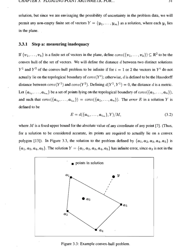
3.3.1 Step a: measuring inadequacy . . .

Vlll 24 24 25

27

TABLE OF CONTENTS

3.3.2 Step b: perturbation analysis . 3.3.3 Step c: stability of algorithms 3.3.4 Consequence . . . .

3.4 Practical implications for three-dimensional applications 3.4.1 A simple application in JR(3: extruded objects 3.4.2 Other problems

3.5 Conclusion References . . . .

4 Reliable joining of surfaces for combined mesh-surface models 4.1 Introduction...

4.2 Error criteria to measure mesh-patch quality 4.3 Joining algorithms . . . .

4.3.1 Whitney extension

4.3.2 Case 1: The bk(t) are provided as input

4.3.3 Case 2: Certain of the bk(t) are not provided as input. 4.3.4 Error estimates

4.4 Computational examples

4.4.1 Examples illustrating the two algorithms 4.4.2 Computational cost .

4.5 Conclusion . . . . 4.6 Acknowledgments References . . . .

S Robustness of Boolean operations on subdivision-surface models 5.1 Introduction...

5.2 Representations of solids 5.3 The Boolean algorithm

5.4 Error estimation and verification of well-formedness 5.4.1 Error estimation . . . . 5.4.2 A posteriori verification of well-formedness . 5.5 Conclusion References . . . . ix 32 32 33 34 34

37

38

38

62

67

79

79

TABLE OF CONTENTS

x

.

List of Figures

1.1 An example of failed convex-hull algorithm. 1.2 An example of a "dirty" geometric mode!.

2.1 Backward/forward error analysis . . . . 2.2 Two adjoining trimmed patches in a surface mode!. 2.3 Subdivision-scheme classifications ..

2.4 Basis function illustration. . 2.5 The Loop subdivision mask. 2.6 The Loop limit-position mask. 2.7 The Loop tangent mask.

2.8 Regularized Boolean operations. 3.1 Well-conditioned problem. 3.2 Ill-conditioned problem. , . 3.3 Example convex-hull problem. 3.4 Overall situation. . . ..

3.5 Simple closed curve formed of Bézier segments (M = 5). 3.6 Extruded object. . . .

4.1 Two adjoining trimmed patches in surface model, with boundary curve b(t), 2 3 8 11 14 15 16 17 17 18 28

29

result of joining. 56

LIST OF FIGURES

4.6 Example with

b(t)

4.7 Input patches with folding present. 4.8 Result with ftipped triangles.

4.9 Sewing result with Whitney extension.

5.1 Subdivision masks (left) and limit mask (right). 5.2 Loop subdivision

.. . . . . .

5.3 Left: a base mesh used to generate the basis functions for the triangle 0-1-2 (regular case: vertex with valence n = 6) [12]; right: the resulting basis function at no de 1 evaluated at subdivision level four.

5.4 (a) control mesh (b) union.

..

5.5 Triangle-triangle intersection ..

5.6 A 2D illustration for the upper and lower bound construction. 5.7 Upper and lower bounds for a single face in the limit mesh. 5.8 Illustration for the tighter bound construction.

. . .

xii 56 57 57 57 68 69 69 70 72 75 76 77

Acknowledgment

1 would like to express my sincere appreciation to Professor Neil F. Stewart, my research super-visor, for his invaluable guidance, his encouragement and his great support throughout aIl the course of the work. Without him this work would not be possible.

1 am particularly grateful to Professor Wolfram Luther for accepting to be my external exam-iner. My thanks also goes to Professor Pierre Poulin and Professor Victor Ostromoukhov for accepting to be the jury members for this thesis.

1 wish to to thank also aIl the people in the Laboratoire d'Infonnatique Graphique de l'Université de Montréal (LIGUM) for the help they offered, the wonderful environment they provided, and aIl the activities we have done together.

FinaIly, 1 wish to express my special acknowledgment to my parents, for their support and encouragement, and my husband, François Duranleau, for his support, his encouragement, his comprehension and his company throughout the years of this work.

Preface

This Ph.D. thesis is a thesis by articles. The main part of the thesis is composed of three accepted (to appear), published, and submitted articles. To better present each individual work, we choose to retain for each paper the complete version as it is (will be) in the respective publication. This leads us to two referencing systems in the thesis. For each paper (Ch. 3, 4, 5), its own references are provided together with the paper: each reference entry is assigned a running number in square brackets as the in-text marker (e.g. [1]). AIso, a bibliography chapter is given at the end of the thesis, and in this case the reference markers are an abbreviation of the authors' name plus year of publication (e.g. [ABA02]). This is the format for the references for aIl the other chapters in the thesis. There are certain overlaps between the bibliography chapter and the references of the three individual articles. Another remark about the bibliography chapter is that the references for websites are given in lowercase, e.g. [g-b].

Chapter 1

Introduction

With the greatly improved computational techniques and the powerful machines available, computer-aided methods have come to be involved in almost every aspect of life:

"Physicists use computers to solve complicated equations modeling everything from the ex-pansion of the universe to the microstructure of the atom, and to test their theories against experimental data. Chemists and biologists use computers to determine the molecular structure of proteins. Medical researchers use computers for imaging techniques and for the statisti-cal analysis of experimental and clinistatisti-cal observations. Atmospheric scientists use numeristatisti-cal computing to process huge quantities of data and to solve equations to predict the weather. Electronics engineers design ever faster, smaller, and more reliable computers using numerical simulation of electronic circuits. Modern airplane and spacecraft design de pends heavily on computer modeling ... " [OveO 1]

In fact, aU fields of science and engineering now rely heavily on numerical computation. But one question has inevitably to be asked: can we trust these numerical computational results?

We do not want our surgery simulation software to turn out to be a source for medical accidents [FGG03]. The following example gives an idea of how bad things can get if not enough attention is given to verification of correctness. Figure 1.1 shows the result of an implemented algorithm for a simple planar convex hull problem1. The point on' the lower left corner which clearly

belongs to the convex hull has been 'ignored, and left outside of the resulting hull. The cause of this failure is the naive use of tloating point arithmetic on a two-dimensional orientation predicate.

lThe convex hull of a finite point set S in the plane is the sma]lest polygon containing the set and such that the vertices of the polygon are points of S [KS86].

1

CHAPTER 1. INTRODUCTION 2

_'1 _ _ _ _ _ _ _ _ _ _ _ _ _ _ _ _ _ _ _

Figure 1.1: An example of failed convex-hull algorithm due to the na ive use of floating-point arithmetic [KMP+04].

Fortunately, numerical non-robustness in scientific computing is a widely recognized phe-nomenon. In particular, the goal of reliable computation has attracted many researchers in the area of geometric modeling.

Two main factors, amongst others, explain the origins of the errors that contribute to nonro-bustness: the use of floating-point arithmetic and uncertainty in the input data. Often, designers of geometric algorithms avoid the problem of computational error by assuming the real random access machine (RAM) as the model of computation [PS85]. The real RAM allows real num-bers to be represented exactly and provides exact arithmetic operations. Unfortunately, often floating-point arithmetic is substituted for exact real arithmetic and special cases are ignored [For93]. Naively applied floating-point arithmetic can cause disastrous results, as illustrated in the previous example (Figure 1.1).

Backward error analysis has become a standard error-analysis method. In the presence of uncertainties in the input data, which is the usual case, it can help to distinguish algorithms that overcome the error problem ta whatever extent it is possible ta do sa. In such situations expensive methods, su ch as exact arithmetic, are not necessary, provided a stable algorithm has been applied. The application of the backward error analysis will pe presented in Ch. 3, with detailed examples provided.

For different geometric problems, non-robustness manifests itself in different manners. The phenomena include random system crashes, inconsistent states (e.g. the geometric data incon-sistent with the topological data), models that contain cracks, holes and overlaps, etc. [YapOl]. This, in tum, means that we have to seek appropriate methods for each problem: a universal solution does not exist. The following example (Fig. 1.2) is a typical "dirty" geometric model:

CHAPTER 1. INTRODUCTION 3 an exterior-mirror model with small cracks (left) , with the zoom-in on the problematic area (middle) and the repaired result (right) [SWCOO].

original model zoom-in of the problem area repaired result Figure 1.2: An example of a "dirty" geometric model [SWCOO].

Depending on the underlying geometric representation used for describing the model, dif-ferent techniques can be used to eliminate the error in the result' each with its own advantages and weaknesses.

NURBS (details in Ch. 2) have bec orne a de facto industry standard for the representation, design, and data exchange of geometric information processed by computer. Trimmed-NURBS (details in Ch. 2) offer greater ftexibility than tradition al NURBS for the design of very sophis-ticated objects, and they have bec orne a very powerful tool used in most commercial model-ing systems. The errors illustrated in Fig. 1.2 may come from inconsistent information, e.g. trimmed-curve mismatch problems. On the other hand, in most cases, for the purpose of ren-dering, the trimmed patches need to be transformed into a polygonal representation. The error, at this stage, may come from the approximation procedure, and a joining (sewing/merging) op-eration can be used to fix the problem. But even in the case that maximum auxiliary information is available, Le. even if we have both trimmed-NURBS and the (triangular) mesh information, a simple joining operation may not produce a satisfying result. Discussion of this problem will be presented in Ch. 4, where an algorithm, which produces a result satisfying two error criteria by using the Whitney extension theorem, will be presented.

NURBS information is not always available in practical applications, e.g. finite-element analysis. Further, a simple polygonal representation (polygon soup) itself is often insufficient for the manipulation of complex geometric models. Therefore, subdivision-surface models (de-tails in Ch. 2) bec orne a convenient representation. In fact, with the increasing popularity of subdivision-surface models, more and more modelers have begun to use them as an

altema-CHAPTER 1. INTRODUCTION 4

tive to trimmed-NURBS, due to their simplicity, generality and efficiency for smooth surface construction [BK04]. Subdivision-surface models do not have the trimming difficulties and the error-prone conversion procedure (from trimmed-NURBS to polygonal meshes) associated with NURBS. Complex models based on subdivision surfaces can be formed using Boolean operations. The related robustness issues of such Boolean operations on subdivision-surface models is the next problem we considered (Ch. 5).

The remainder of the thesis is organized as follows. A short overview of the research area of geometric modeling is given in Ch. 2. It contains two parts: reliable computation (sources of error and error analysis methods), and geometric modelîng, which presents the geometric representations, geometric operations and the related robustness issues. The main part of the thesis (Ch. 3, 4, 5) is composed of three accepted (to appear), published or submitted arti-cles, each of which forms an individual chapter, with a preceding short summary. Chapter 3 describes our work on floating-point arithmetic for computational-geometry problems with un-certain data. Our work on reliable joining of surfaces for combined mesh-surface models is given in Chapter 4. Chapter 5 discusses the problem of robustness of Boolean operations on subdivision-surface models. We conclude in Chapter 6, where we also mention promising pos-sibilities for future work.

Chapter 2

Reliable computation and geometric

modeling

Problems of robustness are a major cause for concem in the implementation of algorithms relat-ing to geometry. Most geometric algorithms are a mix of numerical and combinatorial compu-tations, and the approximate nature of the former often leads to inconsistencies that hinder the ability to construct a satisfactory result [Hof89]. In this chapter an overview of the problems of reliable computation for geometric models will be given, and the related geometric modeling topics, including geometric representations and Boolean operations, will also be presented.

2.1 Finite precision representation and reliable computation

Numerical nonrobustness in scientific computing is a well-known and widespread phenomenon. The root cause is the use of finite-precision numbers, e.g. floating-point representation, to rep-resent real numbers, with precision usually fixed by the machine word size Ce.g. 24 bits). A number of approaches to the finite-precision problem have been advocated in academia. Hoff-mann [HofOl] categorizes these into three strategies: exact arithmetic, symbolic reasoning and interval computation. Exact arithmetic is very expensive, and performance can be badly af-fected if it is used exclusively, so filtered exact arithmetic is usually preferred [SD07]. Another proposed method related to exact arithmetic is the exact geometric computation [Yap06]. Inter-val arithmetic [AH83, Mo066, MB79, Sch99, ELOO, DS88] treats a rounded real number as an interval and the calculations are performed on this interval - but the shortcoming of interval

CHAPTER 2. RELIABLE COMPUTATION AND GEOMETRIC MODELING 6

arithmetic is that it gives overly pessimistic results. Symbolic manipulation is a possible way to avoid rounding and truncation errors. Thus using software such as Mathematica or Maple may be appropriate, but in many application cases, this might not be the best choice for efficiency reasons. Another approach proposed by Yap [YapOl] is exact geometric computation, which again uses approximate arithmetic, but with the level of precision guided by geometric exact-ness. A fifth possibility [HS05, ASZ07] is to use ordinary floating-point arithmetic, and to try to associate the error with the input data. This is appropriate if there is uncertainty in the input.

It is the last mentioned approach that is studied in this work.

2.1.1 Floating-point number system

Floating-point numbers (IEEE 754/854) are the standard substitute for real numbers in scientific computation [OveOl]. Current state-of-the-art CAD (Computer Aided Design) systems used to create and interrogate curved objects are based on geometric solid modeling methods that typically operate using floating-point arithmetic [PM02, PH98, g-L].

A floating-point number system F

c

y

=

±m x

The system F is characterized by four integer parameters • the base (J (sometimes called the radix),

• the precision

t,

• the exponent range emin :::; e :::; e max .

The man tissa m is an integer satisfying 0 :::; m :::; (Jt - 1. To ensure a unique representation for each y E F it is assumed that m

2::

=f

Iyl :::;

The IEEE standard 754/854 for floating-point arithmetic requires that the results of

+, -,

" j, and" are exactly rounded, i.e. the result is the exact result according to the chosen rounding mode. It also specifies floating-point computation in single, single-extended, double, and double-extended precisions. Single precision is specified for a 32 bit word, double precision for two consecutive 32 bit words. In single precision the mantissa length is 24 (including a hidden leading 1 bit) and the exponent range is [-126,127]. Double precision has mantissa length 53 and exponent range [-1022,1023] [Sch99, FGG03].

CHAPTER 2. RELIABLE COMPUTATION AND GEOMETRIC MODELING 7

Floating-point arithmetic has numerous engineering advantages: it is well-supported by programming languages, it is portable, it has useful features such as automatic scaling, and it has been extensively optimized in current computer hardware [For95].

Since an infinite set of numbers is represented by only finitely many floating-point numbers, truncationlrounding techniques have to be used for real numerical values to fit the representation format. Consequently, floating-point computation is, by nature, inexact, and concepts such as representation range, precision and round-off error then arise. Naively applied ftoating-point arithmetic can invalidate axioms of geometry [Sch99]. The paper [00191] and the book by Overton [OveOl] are excellent references for this subject.

2.1.2 Sources of errors

There are three main sources of errors in numerical computation: rounding and truncation due to the finite-precision representation in computer, and data uncertainty [Hig96]. In practice, the input data is often not exact to start with for many applications [Hof89]. Uncertainty may arise in several ways: from error in measuring physical quantities, from errors in storing the data on the computer (truncation errors), or, if the data is itself the solution to another problem, it may be the result of errors in an earlier computation [Hig96]. Another source, additional to the three mentioned, is approximation error, which occurs often in the domain of geometric modeling for practical reasons. One example for this kind of error is the use of low-degree curves to approximate high-degree curves.

2.1.3 Error analysis

The unpredictability of ftoating-point code across architectural platforms in the 1970's and 1980's was resolved through a general adoption of the IEEE standard 754-1985, later enlarged as IEEE standard 854-1987 [OveOl]. But the se standards only make program behavior pre-dictable and consistent across platforms; the errors are still present. Ad hoc methods for fixing these errors (such as treating numbers smaller than sorne positive E as zero) cannot guarantee

their elimination [Yap04]. And since geometric operations usually require extensive numerical calculations, the propagation of the errors is of great concem and profoundly influences the accuracy and validity of the geometric operations [Hof89, MP07]. Therefore, error analysis became very necessary for reliable computation.

re-CHAPTER 2. RELIABLE COMPUTATION AND GEOMETRIC MODELING 8

sulting from the fundamental floating-point arithmetic operations [PM02], especially addition of quantities of opposite sign and approximately equal magnitude: the computed result can be completely wrong due to a simple cancellation (see examples in the paper that follows in Ch. 3).

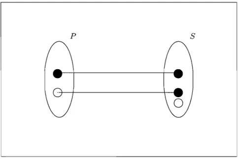
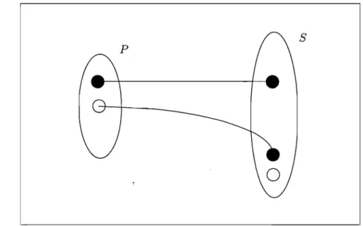
It is often possible to associate the error in a calculation with either the problem or the solution, and there may be sorne choice about how much error is associâted with each of these. Thus, in Fig. 2.1, aIl of the error could be viewed as forward error, with .6.x = 0, or (as illustrated in the figure), part of the error can be associated with the problem. The process of bounding this backward error of a computed solution is called backward error analysis, and its motivation is twofold. First, it interprets rounding errors as being equivalent to perturbations in the data. The input data frequently contains uncertainties due to previous computations or errors committed in storing numbers on the computer, as previously mentioned. If the backward error is no larger than these uncertainties then the computed solution can hardly be criticized - it is as good as we can hope for. The second attraction is this. Rather than viewing aH of the error as forward error, as mentioned just above, the backward error analysis permits to bound or estimate the influence of the total error by means of perturbation theory [DB08].

Figure 2.1: Backwardlforward error analysis, solid line = exact, dashed line = computed.

2.2 Geometrie modeling

Geometric modeling has rapidly bec orne a central area of research and development that in-volves diverse applications. It is of critical importance in the traditional fields of engineering, general product design, and computer-aided manufacturing. It has also proved to be indispens-able in a variety of modern industries, inc1uding computer vision, robotics, medical imaging, visualization, etc. [Sar03].

CHAPTER 2. RELIABLE COMPUTATION AND GEOMETRIC MODELING 9

2.2.1 Historieal summary

Geometric modeling traditionally identifies a body of techniques that can model certain classes of piecewise parametric surfaces, subject to particular conditions of shape and smoothness [G097]. Its beginnings can be traced to the 1950s, and from the se initial activities emerged four main streams of work that evolved largely independently for sorne two or three decades. The computer graphies stream focused on rendering and interaction. The wireframe stream le ad to the commercial CAD systems ofthe 1970s and 80s. Thefree-form curve and surface stream found important applications in computer-aided design and the manufacture of car bodies, air-craft fuselages and in other tasks in the automotive. and aerospace industries. SoUd modeling is distinguished by the use of hopefully unambiguous representations for complete solids. A related fifth stream focuses on the theoretical aspects of design and analysis of geometric al-gorithms, and has bec orne known as computational geometry [Req99]. Since the late 1990s, however, a tendency of convergence of aIl these different aspects of geometric computation has bec orne evident, and new systems use ideas from aIl of these fields [Req99].

2.2.2 Geometrie representations

The development of complex surface representation schemes has been one of the core fields of computer graphics and geometric modeling. The different representations currently available have succeeded in modeling certain properties of surfaces weIl, but none of them is general enough to satisfy aIl the requirements that could be demanded of a representation [HGOO]. Two major representation schema are often used: constructive soUd geometry (CSG) and boundary

representation (B-rep). In CSG a sol id is represented as a set-theoretic Boolean representation of primitive solid objects, so that both the surface and the interior of an object are defined implicitly. In B-rep the solid surface is represented explicitly as a quilt of vertices, edges, and faces [Hof89, G097].

Most geometric modeling systems use B-rep. The different B-rep schemes appearing in the literature can be divided into two major families. One family restricts the solid surfaces to oriented manifolds. The second allows oriented nonmanifolds. Conversion from CSG to B-rep is usually available [G097]. Throughout this work, we focus on the B-rep: three such representations will be presented in detail.

CHAPTER 2. RELIABLE COMPUTATION AND GEOMETRIC MODELING 10

Parame tric representations

Non-Unifonn Rational B-Splines (NURBS) have bec orne a de facto industry standard for the

representation, design, and data exchange of geometric infonnation processed by computer. AIso, many international standards, e.g. STEP Part 42 [Ind97], recognize NURBS as powerful tools for geometric design [PT97]. Their excellent mathematical and algorithmic properties, combined with successful industrial applications, have contributed to the enonnous popularity of NURBS. NURBS also play an important role in the CAD/CAM (Computer-Aided

Manufac-turing)/CAE (Computer-Aided Engineering) world .

A NURBS surface of degree p in the u direction and degree q in the v direction is a bivariate

vector-valued piecewise rational function of the fonn [PT97]

n m

S(u,v)

LLRi,j(U,V)Pi,j

u,v:S 1,

i=ü j=ü

where the

Ri,j (u, v)

n

+

+

R

.. (

) _

Ni,p(u)Nj,q(V)Wi,j

, L..k=ü L..l=ü Nk,p u Nl,q v Wk,l

(2.2)

The

{P i,j}

{Wi,j}

{Ni,p (u)}

{Nj,q( v)}

NURBS provide a convenient way to describe surfaces of almost any shape. However, the most useful NURBS paradigm is constrained by the requirement that the surfaces are defined over rectangular regions and this leads to topologically rectangular patches. A generalization for an arbitrary topology can be obtained by collapsing sorne of the control mesh edges, but this creates surfaces with ambiguous surface nonnals and degenerate parametrization [CMOO].

Trimming operations are essential for modeling non-regular B-rep objects. A trimmed-surface data type in the description of free-fonn objects was therefore introduced to provide

greater power and ftexibility to the NURBS representation. A trimmed surface is an ordinary tensor product surface that has a restricted parameter domain, thus overcoming the limitation of tensor product surfaces defined over rectangular regions, and allowing for arbitrary domains [CMOO]. They can give a complete representation of the boundary of a geometric model by means of union of surfaces restricted to suitable domains.

A trimmed NURBS surface is defined by a tensor product NURBS surface and a set of trimming curves in the parametric space of the surface [CMOO]. The additional trimming

pro-CHAPTER 2. RELIABLE COMPUTATION AND GEOMETRIC MODELING 11

cess, using trimming curves, permits the removal of unneeded areas of the traditional NURBS surface. Combining thousands or even tens of thousands of trimmed surfaces makes it possible to design very sophisticated objects [KBK02].

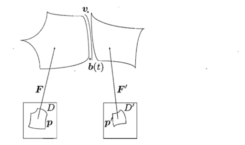
Figure 2.2 gives an example of two trimmed patches joining together to form a single sur-face. The parametric domain D is delimited by a collection of trimming curves p, and the restriction of the mapping F to D defines the trimmed patch in ]R3. In addition, explicit boundary information, provided by a function b(t) taking values in ]R3, may also be present [SWCOO, Spa98, Ind97, KBK02].

Figure 2.2: Two adjoining trimmed patches in a surface model [ASZ07].

Trimmed NURBS surfaces have been adopted widely by the CAD/CAM industry, and in-cluded in graphics standards. They are provided as primitives in several geometric modeling software systems, and the rendering of trimmed NURBS surfaces is supported by international standards, such as STEP Part 42 [Ind97] and PHIGS+ (Programmer's Hierarchi~al Interactive Graphics System), as weIl as graphics programming interfaces, such as OpenGL and Direct3D [CMOO].

Mesh models

NURBS have the advantage of being able to describe almost any shape conveniently. But even today's advanced graphics hardware is unable to directly render trimmed NURBS models: they need to be transformed into a renderable (e.g. polygonal) representation [BGK04, KBK02]. Similarly, for many applications, piecewise linear approximations of smooth surfaces within a given tolerance are generated. Examples of such applications include finite-element analysis, stereolithography, and visualization of geometric models [SBOO]. Many methods have been

CHAPTER 2. RELIABLE COMPUTATION AND GEOMETRIC MODELING 12 proposed in the literature for this triangulation (approximation) procedure [SBOO, Sug02].

A mesh is a discretization of a geometric domain into sm ail simple shapes, such as triangles or quadrilaterals in two dimensions and tetrahedra or hexahedra in three dimensions [BPOO]. Depending on the point of view, meshes can be classified in different ways. Based on topo-logical properties, meshes can be divided into structured meshes 1, unstructured meshes2 and

hybrid meshes3 [GKSS02, BPOO]. Based on the mesh element type, meshes can be categorized into tri/tetrahedral meshes, quadlhexahedra meshes, and others4 [Owe98].

For this Ph.D. work, we focused on triangular-surface meshes, based on the fact that we mainly work on B-rep models, and that triangles are the primitive representation elements for rendering. One of the most popular triangle and tetrahedral meshing techniques is based on the use of the Delaunay criterion, namely the Delaunay triangulation method.

Definition

Let S be a set of points in the plane. A triangulation T is a Delaunay triangulation of S if for each edge e of T there exists a circle C with the following properties [Che89a]:

• the endpoints of edge e are on the boundary of C, and • no other vertex of

S

A circle circumscribing a Delaunay triangle is called a Delaunay circle. If S contains four points that are cocircular then the Delaunay triangulation is not unique [Che89b, ELOO]. In such a circumstance, any of the possible triangulations will do [Che89a]. The Delaunay triangulation is the straight line dual of the Voronoi diagram of S [Che89a].

The Delaunay triangulation has the following properties. Among (aIl triangulations of a vertex set, the Delaunay triangulation maximizes the minimum angle in the triangulation, min-imizes the largest circumcircle, and minmin-imizes the largest min-containment circle, where the min-containment of a triangle is the smallest circle that contains it (and is not necessarily its circumcircle) [She99, DS89, BPOO].

1 Ali interior vertices of the mesh are topologically alike.

2Mesh vertices may have arbitrarily varying local topological neighborhoods.

3The mesh is formed by a number of small structured meshes combined in an overall unstructured pattern. 4This includes mixed tri-quad meshes, mixed tet-hex meshes and other less frequently used element-shape meshes.

CHAPTER 2. RELIABLE COMPUTATION AND GEOMETRIC MODELING 13

Subdivision-surface models

Currently, the most corn mon way to model complex smooth surfaces in the domain of geometric modeling is by using a patchwork of trimmed NURBS. Trimmed NURBS are used' primarily because they are readily available in existing commercial systems such as Autodesk. They do, however, suffer from at least two difficulties [DKT98], which are discussed further in Ch. 4:

• Trimming is expensive and prone to numerical error.

• It is difficult to maintain smoothness, or even approximate smoothness, at the seams of the patchwork when the model is animated.

Subdivision surfaces have the potential to overcome both of these problems: they do not re-quire trimming, and smoothness of the model is automatically guaranteed. Also, subdivision surfaces free the designer from worrying about the topological restrictions that haunt NURBS modelers [DKT98]. Further, compared to the regular mesh models presented in the previous section, subdivision-surface models offer more control over the objects, since they contain more topological and geometrical information about the mesh. But, on the other hand, subdivision-surface models also prevent the use of special tools that have been developed over the years to add features to NURBS models, which is one of the hindrances for the extensive use of subdivision-surface models, especially in the domain of CAD.

Subdivision is a method for generating smooth surfaces, which first appeared as an exten-sion of splines to arbitrary-topology control nets, and was introduced as a generalization of knot insertion algorithms for splines. But it is much more general and offers considerable freedom in the choice of subdivision mIes [Zor97]. Subdivision surfaces were first introduced to the domain of geometric modeling 1978, with the papers by Catmull and Clark [CC78], and by Doo and Sabin [DS78]. Subdivision-surface models are now widely used in many application areas, including computer graphies, solid modeling, computer-game software, film animation and others, as an alternative to B-splines and NURBS [AS09].

The basic idea of subdivision is to define a smooth curve or surface as the limit of a sequence of successive refinements [ZSD+OO]. Most oftenly the subdivision procedure contains two main steps: refinement and smoothing. Refinement (splitting mIe) means splitting the edges and faces by inserting new vertices to obtain a finer version of the mesh, and smoothing (averaging mIe) means shifting the vertices in order to increase the overall smoothness of the surface [AS09, ZSD+OO].

CHAPTER 2. RELIABLE COMPUTATION AND GEOMETRIC MODELING 14

Classification - Many different subdivision schemes have been proposed in the last two decades. Based on different criteria, these schemes can be classified differently. For example, as pro-posed in [AS09], they can be classified according to the type of spline that is generated by the method: B-spline methods, Box-spline methods, general-subdivision-polynomial methods and affine-invariant subdivision methods (Fig. 2.3). Similarly, based on the presence or absence of an interpolating property of the produced surface, subdivision schemes can be categorized as:

interpolating methods (e.g. Modified Butterfly [ZSS96], Kobbelt [Kob96]) and approximating methods (Doo-Sabin [DS78], Catmull-Clark [CC78], Loop [Lo08?], 4-8 [VZ01],

.J3

- Repeated Averaging - Loop - Modified Butterfly - Catmull-Clark - {Midedgep - Kobbelt

- Doo-Sabin - 4-8 subdivision _ {y3}2

- ...

-

..

-

..

-

. ..

t

t

t

Affine-1 1 1

invariant B-spline methods Box-spline methods General- subdivision

subdivision- methods - Lane-Riesenfeld: - Three-direction polynomial

LR(d x d), quartic-spline methods

d

=

-

..

-

- Four -direction - {y3p scheme (x2) -

...

...

Figure 2.3: Subdivision-scheme classifications [AS09].

Surface evaluation - Another important issue conceming subdivision-surface models is surface evaluation. The first evaluation method (other than subdivision refinement itself) was proposed by Stam [Sta98a, Sta98b]: this method parameterizes the control mesh and the limit surface over a unit-mesh element (triangle or quadrilateral) to evaluate the surface at an arbitrary pa-rameter value. Another method was presented in [WP04, WP05, BS02] . It uses the linearity of the subdivision process, the parameterization of the control mesh and the limit surface is set to be centered at each vertex (Fig. 2.4), such that the limit surface is evaluated as the linear combination of the basis functions, weighted by the original control points. One advantage of

CHAPTER 2. RELIABLE COMPUTATION AND GEOMETRIC MODELING 15 this technique is that the parameterization near the extraordinary vertex has n-gon symmetry. It

is the second method that we have used in the paper that follows in Ch. 5.

3~----~~--~-*---~7 3 7

4 5

Figure 2.4: Wu-Peters [WP04] evaluation method: left: a base mesh used to generate the basis functions for the triangle 0-1-2 (regular case: vertex with valence 6); right: the resulting basis function at node 1 evaluated at subdivision level four.

Multiresolution - Multiresolution is a natural extension of subdivision surfaces. It extends sub-division by including detail offsets at every level of subsub-division, unifying patch-based editing with the flexibility of high-resolution polyhedral meshes [ZSD+OO, ZSS97].

Lounsbery et al. were the first to propose algorithms to extend classical multiresolution analysis to arbitrary topology surfaces [Lou94, LDW97]. There are now many different tech-niques available for converting subdivision surfaces into a multiresolution hierarchy [LSS+98]. Two main schools exist. One approach extends classical multiresolution analysis and subdi-vision techniques to arbitrary topology surfaces [Lou94, LDW97, EDD+95, CPD+96]. The alternative is more general and is based on sequential mesh simplification, e.g. progressive meshes [Hop96, HG97]. In either case, the objective is to represent triangulated 2-manifolds in an efficient and flexible way [LSS+98].

For this work we are mostly interested in the triangular B-rep, so we will give more details on the now-classical Loop subdivision scheme. The Loop scheme is a simple approximating face-split scheme for triangular meshes first proposed by Loop [Lo087]. It is based on the three-directional quartic box spline [Bar07], which produces C2_{-continuous surfaces over regular}

meshes. The Loop scheme produces surfaces that are C2-continuous everywhere except at extraordinary vertices, where they are C1-continuous. Later Hoppe et al. [HDD+94] proposed an extension to the Loop scheme with special rules defined for edges to include features such as creases and corners. In [BLZOO], the boundary rules are further improved, and new rules for concave corners and normal modification are proposed. The Loop scheme can be applied to

CHAPTER 2. RELIABLE COMPUTATION AND GEOMETRIC MODELING 16

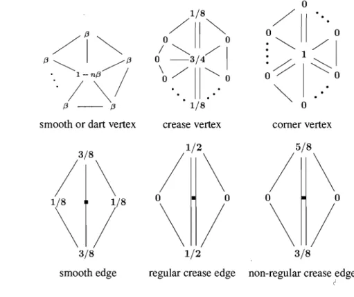
arbitrary polygonal meshes, and the resulting mesh is a triangular mesh [ZSD+OO]. The proof of continuity of this scheme for aIl valences can be found in [Sch96, Zor97]. Below are the three important masks for the Loop subdivision scheme.

1. Subdivision mask

A subdivision mask defines where new vertices will be inserted and how already existing vertices should be shifted at each subdivision step. Fig. 2.5 shows the subdivision mask for Loop subdivision scheme [HDD+94].

/fj~

"~I

/"

'. I - n f j /

.

/~

fj - - fj

smooth or dart vertex

smooth edge

1/8

/~~3~4>ï

\~II~o

_{. .}

1/8

crease vertex corner vertex

regular crease edge non-regular crease edge (

Figure 2.5: The subdivision mask for Loop subdivision scheme, where (3 =

(3(n)

a~),

a(n)

i -

(3+2CO~~27r/n))2.

1-_{n -}(3-~ _n+a(n)'

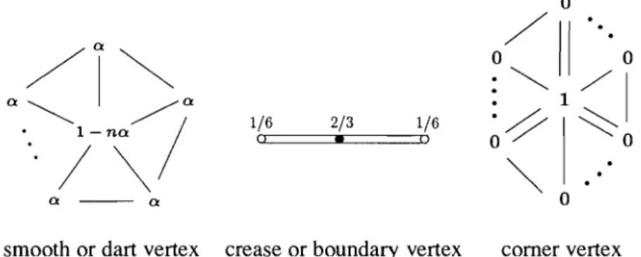
2. Limit mask

A limit mask calculates the limit position of each vertex in the control mesh. The limit position can be expressed as an affine combination of the initial vertex position and its immediate neighboring vertices. For Loop subdivision scheme, this combination is ex-pressed by the following mask (Fig. 2.6) [HDD+94, MMTP04].

CHAPTER 2. RELIABLE COMPUTATION AND GEOMETRIC MODELING Q - - Q 1/6 Il 2/3 • 1/6 l'

smooth or dart vertex crease or boundary vertex corner vertex

17

Figure 2.6: The limit-position mask for Loop subdivision scheme, where a is defined as a =

a(n)

(s'Y(n)

+

n)-l,

,(3)

136'

,(n)

a

+ i

2;)2)

n

Tangent vectors of the limit surface can be computed using the two left eigenvectors of the local subdivision matrix corresponding to the second largest eigenvalues. Then their cross product gives an exact normal vector to the limit surface. For a Loop surface, it can be expressed by the tangent mask (Fig. 2.7) [HDD+94, Kob98].

Cn - - c, C, - - C2

Figure 2.7: The tangent mask for Loop subdivision scheme, where Ci = cos(21fi/n).

2.2.3 Geometrie operations for geometrie models

In most geometric modeling systems, geometric operations can be used to generate free-form models based on sorne primitive models, e.g. the geometric sweep operation [SG05]. Here we give two main groups of these operations .

• Boolean operations

One of the most important facilities of sol id modelers is the Boolean operations between solids [TTSC91, BKZ01]. Regularized Boolean operations inc1ude: regularized union

U*,

n*,

*

op-CHAPTER 2. RELIABLE COMPUTATION AND GEOMETRIC MODELING 18 eration on the interior of the two solids, and they are used to eliminate "dangling" lower-dimensional structures [Hof89]. These operations can be applied to both CSG models and the B-reps5 and include sorne low-level operators as classification, orientation, merging

and intersection.

union

CU*)

cn*)

Figure 2.8: Regularized Boolean operations [g-b].

• Signal processing

Signal processing contains another important group of operations that has been widely used in the domain of geometry processing. It includes downsampling, upsampling,

smoothing [JDD03], filtering [Ale02], etc., which have been used for geometry editing, simplification, denoising, compression and simulation [GSS99]. The paper [BPK+07] gives a nice overview on this subject.

Thn:iughout this Ph.D. work, we put our focus on the Boolean operations on B-reps, al-though other related geometric operations are also studied.

2.2.4 Robustness issues

Boolean operations have been used in most modeling systems, but most often, care still has to be taken to handle special and degenerate cases for these operations [BMS94, TTSC91, BKZOl, Far99]. The inconsistencies arising from numerical error can le ad to connectivity faults, such as breaks in the supposed boundary. And the inaccuracies in the calculations can also create geometric errors, often in the forrn of boundary self-intersections [SD07, Hof89]. In addi-tion, implementation of Boolean operations is especially difficult for higher-order B-reps as it requires intersecting parametric surfaces, separating them into pieces and constructing new sur-faces out of the se pieces. Existing systems typically treat a B-rep as a collection of trimmed

CHAPTER 2. RELIABLE COMPUTATION AND GEOMETRIC MODELING 19

spline patches, sharing boundaries. The boundaries of each individual patch are often matched only approximately, since it is difficult to ensure that two trimming curves in different para-metric domains are identical in space. Thus each intersection operation leads to increasingly complex and difficult-to-handle trimming curves. Applying smooth deformation to the resulting models is also a very difficult task: special care must be taken to avoid cracks, etc. [Man88]. As a result, Boolean operations usually are neither fast nor robust, although excellent results have been achieved by sorne commercial solid modeling engines [LC07, BKZOl, BK97].

The framework necessary to prove that algorithms work rigorously is available [ASZ07], but, so far at least, the required analyses appear to be intractable. Much research has been devoted to seeking robust geometrie-operation algorithms. Two groups of methods have been proposed to repair dirty CAD models: surface-based techniques and volumetrie techniques. Surface-based techniques work directly on the input surface, using different methods to detect and resolve artifacts. These techniques include snapping boundaries to each other, projecting and inserting one boundary into the other, computing intersections of extended surface patches, and propagating the normal field from patch to patch [BK97, BW92, BS95, BDK98, GTLHOI]. The volumetrie technique converts the input into a volumetric representation, effects the repair in the volumetric model and extracts a surface as the final result. It contains different techniques for the B-reps to volumetric representation conversion [NT03, Ju04, FPRJOO], and for the sur-face extractions [KBSS01, Gib98, JLSW02]. AIso, different hole-filling methods have been proposed [BK05, ABA02, DMGL02, NT03] for this volumetric technique. It is the surface-based technique that we will use in the paper in Ch. 5.

Robust operations on subdivision-surface models have recently attracted a lot of attention. Lai and Cheng [LC07, LC06] presented an algorithm that performs error-controllable Boolean operations on Catmull-Clark subdivision-surface models, using a volumetric approach. Lan-quetin et al. [LFKN03] proposed an intersection calculation method for subdivision-surface models based on triangle-grouping technique. Biermann et al. [BKZ01] used a perturbation technique to avoid degenerate cases for Boolean operations on Loop subdivision-surface mod-els. Further Smith and Dodgson [SD07] used symbolic-perturbation methods to guarantee topo-logical correctness of the computed result of Boolean operations. In one of the following papers (Ch. 5), we proposed an algorithm performing Boolean operations on Loop subdivision-surface models using limit-mesh representation, with a verification method designed to guarantee the well-formedness of the computed result.

Chapter 3

Floating-poillt arithmetic for

computational-geometry problems

with uncertain data

This chapter presents our work on the application of backward error analysis in the area of computational geometry. The analysis is relevant in the context of uncertain data, which may weil be the practical context for computational-geometry algorithms.

It has been suggested in the literature that ordinary finite-precision floating-point arithmetic is inadequate for geometric computation, and that researchers in numerical analysis may believe that the difficulties of error in geometric computation can be overcome by simple appioaches. It is our purpose of this work to show that these suggestions, based on an example showing failure of a certain algorithm for computing planar convex hulls, are misleading, and why this is so.

Our exposition illustrates the fact that the backward error analysis does not pretend to over-come the problem of finite precision: it merely provides a tool to distinguish, in a fairly routine way, those algorithms that overcome the problem ta whatever extent it is possible ta do sa. We

also show that the situation in computational geometry, as mentioned in our principal reference [2], is exactly parallel to other areas. For example, algorithms for the planar convex-hull prob-lem were discussed in [2], along with examples of failure of certain of the algorithms. But, although those failures are spectacular, the situation is exactly analogous to many areas of nu-merical analysis: there are certain algorithms that are stable, and certain algorithms that are unstable. If an unstable algorithm is used to solve a problem, then it may produce completely

CHAPTER 3. FLOATING-POINT ARITHMETIC FOR. .. 21 wrong results, and this without warning. On the other hand, if a stable algorithm is applied, then, in the case of problems defined in terms of uncertain data, the algorithm produces an an-swer that is essentially as good as we can hope for. This means, in particular, that one cannot do better by using exact arithmetic.

Three examples (solving linear equations, the planar convex-hull problem and a three-dimensional extruded-objects problem) are then presented to illustrate our method of perform-ing backward error analysis: how to measure the adequacy, how to perform the perturbation analysis and how to seek stable solution methods.

Part of the work was first presented at the Sixth Annual International Workshop on Compu-tatiOnal Geometry and Applications, Glasgow, UK, May 8-11, 2006, and it appeared in Lecture Notes in Computer Science LNCS3980, pages 50-59, 2006. We also invited the authors of our

main reference [2] to reply to our paper; the reply is published together with our initial paper in the LNCS volume [KMP+06]. It is an interesting discussion that shows different points of view concerning the same problem in different research domains. The extended version of the paper presented here, which shows how the results apply in a simple three-dimensional case, will appear in the International Journal of Computational Geometry and Applications.

The main contributions of this work are:

• we show that the numerical difficulties described in the principal reference [2] are unex-ceptional.

• we show how to perform perturbation analysis in geometry modeling with three exam-pIes.

CHAPTER 3. FLOATING-POINT ARITHMETIC FOR. ..

Floating-point arithmetic for computational-geometry

problems with uncertain data

D.

F.

Département d'informatique et de recherche opérationnelle Université de Montréal

to appear in

International Journal of Computation al Geometry and Applications

22

lThe research of the second author was supported in part by a grant from the Natural Sciences and Engineering Research Council of Canada.

CHAPTER 3. FLOATING-POINT ARITHMETIC FOR. .. 23

Abstract

It has been suggested in the literature that ordinary finite-precision f1oating-point arithmetic is inadequate for geometric computation, and that researchers in numerical analysis may believe that the difficulties of error in geometric computation can be overcome by simple approaches. It is the purpose of this paper to show that the se suggestions, based on an example showing failure of a certain algorithm for computing planar convex hulls, are misleading, and why this is so.

It is first shown how the now-classical backward error analysis can be applied in the area of computational geometry. This analysis is relevant in the context of uncertain data, which may weIl be the practical context for computational-geometry algorithms such as, say, those for computing convex hulls. The exposition will illustrate the fact that the backward error analysis does not pretend to overcome the problem of finite precision: it merely provides a way to distinguish those algorithms that overcome the problem ta whatever extent it is possible ta do sa.

It is th en shown that often the situation in computational geometry is exactly parallel to other areas, such as the numerical solution of linear equations, or the algebraic eigenvalue problem. Indeed, the ex ample mentioned can be viewed simply as an example of the use of an unstable algorithm, for a problem for which computational geometry has already discovered provably stable algorithms.

FinaIly, the paper discusses the implications of the se analyses for applications in three-dimensional solid modeling. This is done by considering a problem defined in terms of a simple extension of the planar convex-hull algorithm, namely, the verification of the well-formedness of extruded objects. A brief discussion conceming more difficult problems in solid modeling is also included.

Keywords:

f1oating-point arithmetic, robustness in geometric computation, stability, pl anar convex hull, backward error analysis.