Skewness Risk and Bond Prices
Francisco Ruge-Murcia
May 2012
Abstract
Statistical evidence is reported that even outside disaster periods, agents face neg-ative consumption skewness, as well as positive in ation skewness. Quantitneg-ative im-plications of skewness risk for nominal loan contracts in a pure exchange economy are derived. Key modeling assumptions are Epstein-Zin preferences for traders and asym-metric distributions for consumption and in ation innovations. The model is solved using a third-order perturbation and estimated by the simulated method of moments. Results show that skewness risk accounts for 6 to 7 percent of the risk premia depending on the bond maturity.
JEL Classi cation: E43, G12
Key Words: Term structure of interest rates; bond premia, nonlinear dynamic models; simulated method of moments.
Departement de sciences economiques and CIREQ, Universite de Montreal. I thank the Social Sci-ences and Humanities Research Council of Canada for nancial support. Correspondence: Department of Economics, University of Montreal, C.P. 6128, succursale Centre-ville, Montreal (Quebec) H3C 3J7, Canada.
1
Introduction
This paper is concerned with the pricing of nancial instruments|in particular, nominal loans|in an environment where traders face skewness risk. By skewness risk, I mean the possibility of extreme realizations from the long tail of an asymmetric shock distribution. As an example, suppose that in ation surprises are positively skewed and, thus, during the bond holding period a large positive in ation realization is possible, but a large negative realization is unlikely. Since the former event reduces the real payo of the one-period bond and the real price of longer-term bonds, a trader interested in buying nominal bonds may require compensation for such risk. Similarly, if consumption surprises are negatively skewed, a trader who uses the bond market to transfer resources intertemporally and smooth consumption would consider the eventuality of a large decrease in consumption when settling the price of the asset.
I explore the relation between skewness risk and bond prices using the simplest possible environment: a consumption-based asset-pricing model where traders receive a stochastic, non-storable endowment in every period and there are no frictions. Traders have recursive preferences of the form proposed by Epstein and Zin (1989). Crucially, I relax the usual assumption of that shock innovations follow a symmetric distribution (e.g., normal) and allow instead skewed distributions for the innovations of the in ation and consumption processes. I show that a third-order perturbation of the policy functions that solve the full dynamic model explicitly captures the contribution of skewness to bond yields, prices, and risk premia, and permit the construction of model-based estimates of the e ect of skewness risk on these variables.
The third-order perturbation of the model is estimated by the simulated method of moments (SMM) using quarterly U.S. data. Among the estimated parameters are the ones of the distributions that generate in ation and consumption innovations. Based on these estimates, I statistically show that the data decisively reject the assumption that shock innovations are drawn from normal distributions and favor instead the alternative that they are drawn from asymmetric distributions. In particular, the data prefer a speci cation where in ation innovations are drawn from a positively skewed distribution, and consumption innovations are drawn from a negatively skewed distribution.
The quantitative analysis of the model indicates that most of the bond premia is driven by variance risk, but that skewness risk nonetheless accounts for 6 to 7 percent of the premia depending on the bond maturity. Regarding bond prices, results indicate that in the exchange economy, skewness risk increases the price of a bond that pays 1 unit of currency at maturity by 0.03 cents in the case of the 1-period bond and 0.23 cents in the case of the
8-period bond. In terms of yields, this translates into a reduction of 0:11 percentage points at the annual rate for the 1-period bond and 0:09 percentage points for the 8-period bond.
Impulse-response analysis shows that positive in ation shocks reduce bond prices and increase yields with quantitatively di erent e ects across maturities: the e ect on prices increases monotonically with the maturity while that on yields decreases monotonically. Negative in ation shocks have the opposite e ects. Furthermore, the e ect of positive and negative in ation shocks are asymmetric. For example, a positive shock in the 95th percentile delivers much larger responses than the equally-likely negative shock in the 5th percentile. Positive consumption shocks increase bond prices and reduce yields with the opposite e ects for negative shocks. Again, e ects are asymmetric in that negative shocks induce larger responses than equally-likely positive shocks. Results also show that in ation shocks change the slope of the yield curve because they a ect more short-term than long-term maturities. Consumption shocks a ect all yields almost equally and, hence, push the whole yield curve up or down. Thus, in the exchange economy, in ation acts like the \slope" factor, and con-sumption acts like the \level" factor, in factor models of the term structure. However, while the macroeconomic content of statistical factors is unclear, the \factors" in the exchange economy are the state variables of the model, namely aggregate consumption and in ation. This paper complements the growing literature that studies the e ects of consumption disasters on asset prices, for example Rietz (1988), Barro (2006, 2009), and Barro et al. (2010). Disasters are extreme, low probability events where output (or consumption) drops by at least 15 percent from peak to trough as, for example, during the Great Depression. Under an empirically plausible parameterization of the disaster probability, disasters can help account for the equity premium puzzle. As that literature, this paper is concerned with asymmetries in consumption growth. However, I provide statistical evidence that, even outside disaster events, consumption innovations are negatively skewed and, hence, agents face the possibility of substantial decreases in consumption. Parameter estimates imply that agents can su er a reduction in consumption of 5 percentage points below the mean with a probability 2.6 percent. Of course, these decreases are not as dramatic as disasters and are instead primarily associated with recessions, but they are shown to have a non-negligible e ects on bond prices and risk premia. Moreover, while the disaster literature is primarily concerned with consumption, this paper also considers asymmetries in aggregate in ation, which turn out to be important for the pricing of nominal assets.
This paper also complements the nance literature concerned with the role of skewness in explaining the cross-section of stock returns. Mandelbrot and Hudson (2004) forcefully argue against the unrealistic assumption of normality, which ignores thick tails and skewed realizations in asset prices. Kraus and Litzenberger (1976, 1983) extend the capital asset
pricing model (CAPM) to incorporate the e ect of skewness on valuations. Harvey and Siddique (2000) study the role of the co-skewness with the aggregate market portfolio and nd a negative correlation between co-skewness and mean returns. Kapadia (2006) and Chang et al. (2012) nd that market skewness risk has a negative e ect on excess returns in a cross-section of stock returns and option data, respectively. Papers that examine the role of preferences in accounting for the empirical importance of skewness include Golec and Tamirkin (1998) and Brunnermeier et al. (2007). Golec and Tamarkin estimate the payo function of bettors in horse tracks and nd that it is decreasing in the variance but increasing the skewness, so that at high odds, bettors are willing to accept poor mean returns and variance because the skewness is large. Brunnermeier et al. develop a model of optimal beliefs which predicts that traders will overinvest in right-skewed assets.
The paper is organized as follows. Section 2 describes an exchange economy subject to asymmetric consumption and in ation shocks. Section 3 describes the data, outlines the econometric approach used to estimate the model, reports parameter estimates, and discusses identi cation. Section 4 reports implications for the yield curve, the unconditional skewness of macro variables, and volatility clustering. Section 5 quanti es the contribution of skewness risk to the bond premia and its e ect on bond prices and yields in the exchange economy. Section 6 uses impulse-response analysis to study the e ects of in ation and consumption shocks on bond prices and yields. Finally, Section 7 concludes and outlines my future research agenda on skewness risk.
2
An Exchange Economy
The economy consists of identical, in nitely-lived traders whose number is normalized to 1. The representative trader has recursive preferences (Epstein and Zin, 1989),
Ut= (1 ) (ct)1 1= + Et Ut+11
(1 1= )=(1 ) 1=(1 1= ))
; (1)
where 2 (0; 1) is the discount factor, ct is consumption, Et is the expectation conditional
on information available at time t, is the intertemporal elasticity of substitution, and is the coe cient of relative risk aversion. As it is well known, recursive preferences decouple elasticity of substitution from risk aversion when 6= 1= , and encompass preferences with constant relative risk aversion when = 1= . Previous literature that employs recursive preferences in consumption-based models of bond pricing include, among others, Epstein and Zin (1991), Gregory and Voss (1991), Piazzesi and Schnider (2007), Doh (2008), van Binsbergen et al. (2010), Le and Singleton (2010), and Rudebusch and Swanson (2012).
In every period, the trader receives a non-storable endowment, yt, that follows the process
ln(yt) = (1 ) ln(y) + ln(yt 1) + t; (2)
where 2 ( 1; 1), ln(y) is the unconditional mean of ln(yt), and t is an independent and
identically distributed (i:i:d:) innovation with mean zero, constant conditional variance, and non-zero skewness. The latter assumption relaxes the usual restriction of zero skewness implicit in most of the previous literature (for example, through the assumption of normal innovations),1 and allows me to examine the relation between skewness risk and asset prices. The nancial assets in this economy are zero-coupon nominal bonds with maturities ` = 1; : : : ; L: All bonds are equally liquid regardless of their maturity and can be costlessly traded in a secondary market. The trader's budget constraint is
ct+ L X `=1 Q` tBt` Pt = yt+ L X `=1 Q` 1t B` t 1 Pt ; (3) where Q`
t and Bt` are, respectively, the nominal price and quantity of nominal bonds with
maturity `, and Pt is the price level. Prices are denominated in terms of a unit of account
called \money", but the economy is cashless otherwise.
The Euler equations that characterize the trader's utility maximization are
Q`t Pt = Et vt+1 wt 1= c t+1 ct 1= Q` 1 t+1 Pt+1 !! ; for ` = 1; 2; :::L; (4) where vt max fct;Bt1;:::;BtLg Ut and wt Etvt+1
are the value function and the certainty-equivalent future utility, respectively. As usual, Euler equations compare the marginal cost of acquiring an additional unit of the nancial asset with the discounted expected marginal bene t of keeping the asset till next period.
Euler equations of this form have been extensively studied in the asset-pricing litera-ture. One approach involves estimating the parameters using, for example, the generalized method of moments and testing the over-identifying restrictions of the model. Well-known
1An important exception is the disaster literature (e.g., see Barro, 2006) where innovations are drawn from
the mixture of a normal distribution, that describes non-disaster periods, and a Bernoulli distribution, that can generate a disaster with a xed probability. This combination delivers a negatively skewed distribution. Estimates reported below will statistically support the view that, even outside disaster periods, consumption innovations are negatively skewed, while in ation innovations are positively skewed, and, hence, agents still face skewness risk.
examples are Hansen and Singleton (1982) for expected utility, and Epstein and Zin (1991) for non-expected utility. Another approach involves assuming that the arguments inside the expectations operator are jointly lognormal and conditionally homoskedastic in order to obtain a tractable linear speci cation of the pricing function with a risk-adjustment factor, as in Hansen and Singleton (1983), Campbell (1986, 1996), and Jerman (1998). Since the risk-adjustment factor is constant, this approach rules out the time-variation in risk pre-mia documented, among others, by Cochrane and Piazzesi (2005). Also, since the factor is proportional to the variance of the innovations only, this approach assumes away the con-tribution of higher-order moments, like skewness, to the risk premia. In contrast, the focus of this paper is on the policy functions that solve the full dynamic model, rather than on the Euler equations alone. As we will see, policy functions are useful characterizations of prices and quantities because they make explicit their dependence on the state variables of the model and on the higher-order moments of the innovations.2
The model is closed by assuming that aggregate in ation follows the process3
ln ( t) = (1 ) ln( ) + ln( t 1) + t; (5)
where t = Pt=Pt 1 is the gross rate of in ation between periods t 1 and t, 2 ( 1; 1),
ln( ) is the unconditional mean of ln( t), and t is an i:i:d: disturbance with mean zero,
constant conditional variance, and non-zero skewness.
The equilibrium is an allocation for the traderC = ct; Bt` `=1;::L 1 t=0
and a price system
n
(Q` t)`=1;::L
o1
t=0 such that given the price system: (i) the allocation C solves the trader's
problem; (ii) the goods market clears: Ct = Yt; and (iii) bonds are in zero net supply:
Bt` = 0 for all ` = 1; 2; :::; L.
Note that the assumption of a representative trader and the normalization of the popula-tion size to 1 means that, in equilibrium, aggregate consumppopula-tion and output are respectively equal to the individual consumption and endowment. That is, Ct = ct and Yt = yt. With
the understanding that Ct = yt in equilibrium only, I will refer to (2) as the consumption
process.
I now derive the relation between the bond prices determined by the model, and the bond
2Martin (2012) relaxes the assumption of lognormality and expresses variables (e.g., the riskless rate) as
polynomial functions of consumption growth cumulants. Similarly, the perturbation method that I use here to solve the model allows the higher-order moments of consumption, as well as in ation, to a ect the model variables.
3In preliminary work, I explored another strategy to close the model. That is, by using an autoregressive
process for the growth rate of the money supply to represent monetary policy, and specifying real money balances as one of the arguments in the utility function. However, when I estimated this version of the model, I found a relatively low interest rate elasticity of money demand. Coupled with exible prices, this is equivalent to, but less parsimonious than, directly assuming a time-series process for in ation.
yields and risk premia. These derivations are relatively standard and the intention is simply to be explicit about the variables I will be focusing on in the empirical part of the paper. Following the literature, the gross yield of the `-period bond is
i`t = Q`t 1=`; (6)
for ` = 1; 2; :::; L. The bond risk premium (or bond premium for short) is the component of the long-term bond price that accounts for the risk involved in holding this bond compared with a sequence of rolled-over shorter-term bonds. The risk arises because future bond prices are not known in advance and, so, the strategy of rolling over shorter-term bonds entails a gamble. I derive the bond premium recursively from the Euler equations
Q`t = Q1tEt Q` 1t+1 + covt Vt+1 Wt 1= Ct+1 Ct 1= ;Q ` 1 t+1 t+1 ! ; (7)
for ` = 2; :::L, where Vt and Wt are, respectively, the aggregate counterparts of vt and wt,
and I have used the fact that for the one-period bond
Q1t = Et Vt+1 Wt 1= C t+1 Ct 1= 1 t+1 ! : (8)
Following Ljungqvist and Sargent (2004, ch. 13.8), the premium on the `-period bond is de ned as `;t covt Vt+1 Wt 1= C t+1 Ct 1= ;Q ` 1 t+1 t+1 ! : (9)
Notice that the premium depends on the bond maturity and may be positive or negative according to the sign of the covariance between the pricing kernel and Q` 1t+1= t+1. This
observation highlights the fact that, in general, consumption-based asset-pricing models do not restrict the sign or monotonicity of the bond premia. The same is true in the market-segmentation hypothesis by Culbertson (1957) and the preferred-habitat theory by Modigliani and Sutch (1966), but they rely on a strong preference by investors for particular maturities and, implicitly, rule out arbitrage.
Using de nition (9), the price of the `-period bond can be written as
Q`t = Q1tEt Q` 1t+1 + `;t: (10)
From de nition (9), the premium is negative when the covariance in (9) is negative. A negative premium implies Q`
t < Q1tEt Q` 1t+1 , meaning that buying a `-period bond at time
t is cheaper than buying a one-period bond at time t and a (` 1)-period bond at time t + 1. Up to an approximation, this implies that the yield of the `-period bond is larger than the
weighted average yield of the 1- and (` 1)-period bonds and the yield curve is, therefore, upward sloping.4 Conversely, the premium is positive when the covariance in (9) is positive
and the yield curve is downward sloping.
Since this model does not have an exact analytical solution, I use a perturbation method to obtain an approximate solution (see Jin and Judd, 2002). This method involves taking a third-order expansion of the policy functions around the deterministic steady state and characterizing the local dynamics. An expansion of (at least) third-order is necessary to cap-ture the e ect of skewness in the policy functions and to generate a time-varying premium.5 Caldera et al. (2009) show that for models with recursive preferences, a third-order pertur-bation is as accurate as projection methods (e.g., Chebychev polynomials and value function iteration) in the range of interest while being much faster computationally. The latter is an important advantage for this research project because estimation requires solving and simulating the model in each iteration of the routine that optimizes the statistical objective function.
A policy function takes the general form f (xt; ) where xt is a vector of state variables
and is a perturbation parameter. The goal is to approximate f (xt; ) using a third-order
polynomial expansion around the deterministic steady state where xt = x and = 0. Using
tensor notation, this approximation can be written as
[f (xt; )]j = [f (x; 0)]j + [fx(x; 0)]ja[(xt x)]a (11) +(1=2)[fxx(x; 0)] j ab[(xt x)]a[(xt x)]b +(1=2)[f (x; 0)]j[ ][ ] +(1=6)[fxxx(x; 0)]jabc[(xt x)]a[(xt x)]b[(xt x)]c +(1=2)[fx (x; 0)]ja[(xt x)]a[ ][ ] +(1=6)[f (x; 0)]j[ ][ ][ ];
where I have used [fx (x; 0)]ja = [f x(x; 0)]ja = 0 (Schmitt-Grohe and Uribe, 2004, p. 763),
[fxx (x; 0)]jab = [f xx(x; 0)]jab = [fx x(x; 0)]jab = 0 (Ruge-Murcia, 2012, p. 936), and [f x(x; 0)]ja
4To see this, consider the simplest case where ` = 2. Then, using (6) for ` = 1; 2, it is easy to show that
Q2
t < Q1tEt Q1t+1 implies log(i2t) > (1=2)(log(i1t) + Et log(i1t) . This mechanism is di erent from the one
outlined by Hicks (1939, ch. 13) where long-term bonds are \less liquid" than short-term bonds and, hence, a premium is required to induce traders to hold the former. Instead, in this model all bonds are equally liquid and can be traded without penalty before their maturity date. Bansal and Coleman (1996) assume that short-term bonds provide indirect transaction services and the compensation for those services lowers the nominal return of short-term bonds compared with long-term bonds.
5As it is well known, rst-order solutions feature certainty equivalence and imply that traders are
indif-ferent to higher-order moments of the shocks. Second-order solutions capture the e ect of the variance, but not of the skewness, on the decision rules, and deliver a constant risk premium. For the implementation of the third-order perturbation, I use the codes described in Ruge-Murcia (2012).
= [f x (x; 0)]ja = [fx (x; 0)]ja by Clairaut's theorem. As we can see, the function includes
linear, quadratic, and cubic terms in the state variables, one constant and one time-varying term in the variance, and one constant term in the skewness. In the special case where the distribution of the innovations is symmetric|and, hence, skewness is zero|the latter term is zero. In the more general case where the distribution is asymmetric, this term may be positive or negative depending on the sign of the skewness and the values of other structural parameters.
The state variables in this exchange model are aggregate consumption and in ation, that is, xt = [Ct t]0. The reader familiar with recent contributions to the macro- nance
literature will notice that the policy functions of yields and the pricing kernel, written in the generic form (11), resemble the basic equations of the canonical factor model of the term structure. However, there are four important di erences. First, the factors here are observable macroeconomic variables, rather than latent variables. Latent factor models suggest the existence of two key factors, namely the \level" and \slope" factors, which jointly account for 95 percent of the variance of yields (Rudebusch and Wu, 2008, p. 909). However, given the purely statistical nature of those models, the macroeconomic content of the factors is unclear. In this model, their macroeconomic interpretation is explicit: the factors are aggregate consumption and in ation. Furthermore, as we will see below, the relation between the level and slope factors and the state variables of the model is empirically straightforward.6
Second, the function is not a ne but non-linear as a result of the quadratic and cubic terms that arise from the third-order perturbation. Le and Singleton (2010) build a factor model where the price/consumption ratio is a quadratic function of the state variables, but a suitable linearization renders the model conditionally a ne. Third, since innovations are drawn from an asymmetric distribution, this model is not Gaussian. Finally, while the factor loadings are typically free parameters in statistical factor models, in this model the coe cients of the state variables are non-linear functions of structural parameters.
6Papers that attempt to build a tighter link between latent and macroeconomic factors include Ang and
Piazzesi (2003), Diebold et al. (2006), Wu (2006), and Rudebusch and Wu (2008). Ang and Piazzesi, and Diebold et al. specify factor models where the state vector consists of a mix of latent variables and macro-economics variables. In the former case, the macroeconomic variables are the rst principal components of various in ation and output measures. In the latter case, the macroeconomic variables are in ation, capacity utilization, and the federal funds rate, with possible feedback from latent variables to macro variables. Wu nds that in a calibrated New Keynesian model, monetary policy shocks explain most of the slope changes in the term structure, while technology shocks explain most of the level changes. Rudebusch and Wu build a model where two latent factors are respectively driven by the central bank's in ation target and reaction function.
3
Econometric Analysis
3.1
Data
The third-order approximate solution of the model is estimated using quarterly observa-tions of the growth rate of consumption, the in ation rate, and the three-month, six-month, and twelve-month nominal interest rates. The raw data were taken from the FRED data-base available at the Web site of the Federal Reserve Bank of St. Louis (www.stls.frb.org). Consumption is measured by personal consumption expenditures on non-durable goods and services, which were converted into real per-capita terms by dividing by the quarterly aver-age of the consumer price index (CPI) for all urban consumers and by the quarterly averaver-age of the mid-month U.S. population estimate produced by the Bureau of Economic Analysis (BEA). In order to assess the robustness of the results to the consumption measure, I also estimate the model using personal consumption expenditures on non-durable goods only.
Since a period in the model is one quarter, the three-month Treasury Bill rate serves as the empirical counterpart of the one-period nominal interest rate. The six-month and twelve-month rates are the two-period and four-period interest rates, respectively. Note that the three-, six-, and twelve-month Treasury bills have, in fact, maturities of thirteen, twenty-six, and fty-two weeks, respectively. Rather than averaging the Treasury Bill rates over the quarter, I used the observations for the rst trading day of the second month of each quarter (that is, February, May, August and November). Treasury Bills are ideal for this analysis because, like the bonds in the model, they are zero-coupon bonds with negligible default risk. The original interest rate series, which are quoted as a net annual rate, were transformed into a gross quarterly rate. Except for the nominal interest rates, all raw data are seasonally adjusted at the source. The sample period is from 1960Q1 to 2001Q2, with the latter date determined by the availability of the twelve-month Treasury Bill rate.7
7The U.S. Treasury stopped reporting secondary market yields for this Bill after 27 August 2001. The
Board of Governors of the Federal Reserve also publishes \constant maturity" yields for Treasury securities with maturities of one year and more. These yields are constructed by the U.S. Treasury using a polynomial interpolation from the yield curve of actively traded Treasury notes and bonds. In preliminary work, I considered using these yields for the model estimation, but abstained from doing so for two reasons. First, Treasury notes and bonds pay coupons and are, therefore, not directly comparable to the bonds in the model. Second, and more importantly, these yields are constructed, rather than observed, and may correspond to securities that were not available for trading at a given date. This concern applies more generally to other constructed series, like the CRSP Fama-Bliss discount bond series. When I compared the 12-month Treasury bill and 1-year constant-maturity rates, I found that although they are highly correlated, the bill rate is almost always below the constant rate and the average di erence is large: about 42 basis points at the annual rate. In certain periods (for example, in mid-May 1981), the di erence was as large as 200 basis points.
3.2
Estimation
The model is estimated by the simulated method of moment (SMM). The SMM estimator minimizes the weighted distance between the unconditional moments predicted by the model and those computed from the data, where the former are computed on the basis of arti cial data simulated from the model. Lee and Ingram (1991) and Du e and Singleton (1993) show that SMM delivers consistent and asymptotically normal parameter estimates under fairly general regularity conditions. Ruge-Murcia (2012) explains in detail the application of SMM for the estimation of non-linear dynamic models and provides Monte-Carlo evidence on its small-sample properties.
More formally, de ne 2 to be a q 1 vector of structural parameters with <q,
mt to be a p 1 vector of empirical observations on variables whose moments are of our
interest, and m ( ) to be the synthetic counterpart of mt whose elements are obtained from
the stochastic simulation of the model. The SMM estimator, b, is the value that solves min f g M( ) 0WM( ); (12) where M( ) = (1=T ) T X t=1 mt (1= T ) T X =1 m( );
T is the sample size, is a positive constant, and W is a q q weighting matrix. Under the regularity conditions in Du e and Singleton (1993),
p T (b )! N(0;(1 + 1= )(J0W 1J) 1J0W 1SW 1J(J0W 1J) 1); (13) where S = lim T !1V ar (1= p T ) T X t=1 mt ! ; (14)
and J = E(@m ( )=@ ) is a nite Jacobian matrix of dimension p q and full column rank. In this application, the weighting matrix is the diagonal of the inverse of the matrix with the long-run variance of the moments, which was computed using the Newey-West estimator with a Barlett kernel and bandwidth given by the integer of 4(T =100)2=9 where T = 166 is the sample size. The number of simulated observations is ve times larger than the sample size.8 The dynamic simulations of the non-linear model are based on the pruned version of
the solution, as suggested by Kim et al. (2008).
8Ruge-Murcia (2012) performs experiments using simulated samples that are ve, ten, and twenty times
larger than the sample size. Results indicate that the former ( ve) is much more computationally e cient, and only slightly less statistically e cient, than the larger values (ten and twenty).
An important part of this research project involves relaxing the assumption that shock innovations are drawn from a symmetric distribution. In symmetric distributions the shape of the right side of the central maximum is a mirror image of the left side. Loosely speaking, this means that positive realizations of a given magnitude are as likely as negative realizations. As pointed out above, symmetric distributions rule out skewness risk by construction.
Instead, I assume here that innovations are drawn from a skew normal distribution. This asymmetric distribution is characterized by three parameters|a location, a scale, and a cor-relation parameters|and it is attractive for several reasons. First, its support is ( 1; +1), while other asymmetric distributions (e.g., the chi-squared and Rayleigh distributions) have support on [0;1) only, which is restrictive for this application. Second, it can accommodate both positive and negative skewness depending on the sign of the correlation parameter. Finally, it nests the normal distribution as a special case when the correlation parameter is zero. This means that it is straightforward to test the hypothesis that innovations are drawn from a (symmetric) normal distribution against the alternative that they are drawn from an (asymmetric) skew normal distribution. This simply involves performing the two-sided t-test of the hypothesis that the correlation parameter is zero against the alternative that it is di erent from zero.
The moments used to estimate the model are the variances, covariances, skewness, and rst-order autocovariances of all ve data series, and the unconditional means of in ation and the nominal interest rates. I estimate ten structural parameters: the discount factor ( ), the intertemporal elasticity of substitution ( ), the coe cient of relative risk aversion ( ), the rate of in ation in the deterministic steady state ( ), and the autoregressive coe cients and the correlation and scale parameters of the innovation distributions of in ation and consumption. During the estimation procedure, the location parameter was adjusted so that the mean of the innovations is zero, and the unconditional mean of the endowment process was normalized to 1. Since I use twenty-nine moments to estimate ten parameters, the degrees of freedom are nineteen.
3.3
Parameter Estimates
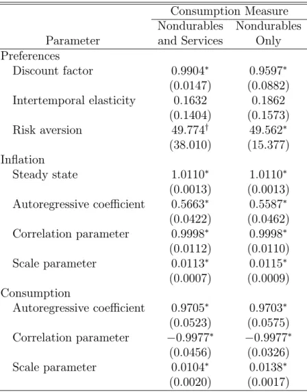
SMM estimates of the parameters of the model, with consumption measured by expenditures on non-durable goods and services, are reported in column 1 of table 1.
The discount factor is 0.99, which implies an annualized gross real interest rate of 1.04 in the deterministic steady state. The intertemporal elasticity of substitution is quantitatively low (0.16) and statistically less than 1. This estimate is in line with values reported in earlier literature. For example, Hall (1988) reports estimates between 0.07 and 0.35; Epstein and
Zin (1991) report estimates between 0.18 and 0.87 depending on the measure of consumption and instruments used; and Vissing-J rgensen (2002) reports estimates between 0.30 and 1 depending on the households' asset holdings.
The coe cient of relative risk aversion is about 50, which is of the same order of mag-nitude as the estimate of 79 reported by van Binsbergen et al. (2010). In some sense, these relatively high estimates of the coe cient of relative risk aversion are not surprising because previous calibration studies that use Epstein-Zin preferences (e.g., Tallarini, 2000, and Rudebusch and Swanson, 2012) nd that large risk aversion is necessary to match the
rst-order moments of asset returns.
The in ation rate is mildly persistent and the correlation parameter is positive, meaning that in ation innovations are positively skewed. That is, their distribution has a longer tail on the right, than on the left, side, and the median is below the mean. Since the correlation parameter is statistically di erent from zero, the null hypothesis that in ation innovations are drawn from a normal distribution can be rejected in favor of the alternative that they are drawn from an asymmetric skew normal distribution with positive skewness (p-value < 0:001). This result is relevant for future empirical research in macroeconomics and nance, and supportive of Mandelbrot and Hudson (2004), who advocate relaxing the restrictive assumption of normality in favor of more general statistical distributions.
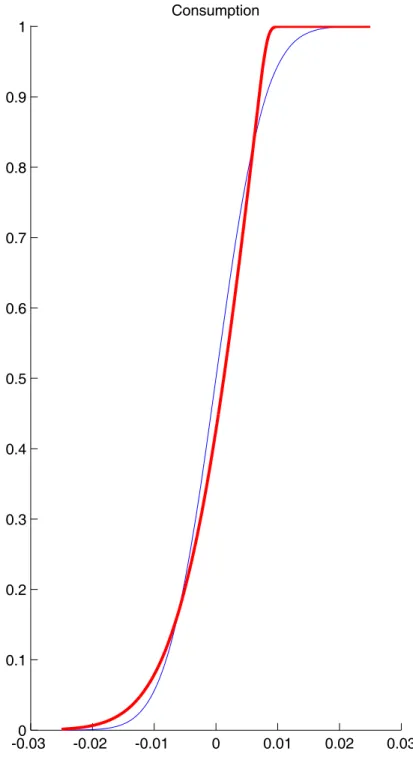
Panel A in gure 1 plots the estimated cumulative distribution function (CDF) of the in ation innovations and compares it with the CDF of a normal distribution with the same variance. Note that the skew normal CDF has more probability mass in the right tail, and less mass in the left tail, than the normal distribution. Thus, loosely speaking, large positive in ation surprises can happen sometimes, but large negative ones are unlikely. This means that, for a given variance, the buyer of a nominal bond faces the risk of large realizations from the right tail of the in ation distribution, which reduce the real price of bonds with maturity larger than 2 periods and the real payo of the bond with maturity equal to 1 period.
The consumption process is very persistent and the correlation parameter is negative. The latter nding implies that consumption innovations are negatively skewed. Hence, their distribution has a longer tail on the left, than on the right, side, and the median is above the mean. The literature on consumption disasters also features a negatively skewed distri-bution arising from the combination of a normal distridistri-bution for non-disaster periods and a Bernoulli distribution that generates disasters. Interestingly, the correlation parameter for consumption innovations in table 1 is statistically di erent from zero. This implies that the null hypothesis that consumption innovations are drawn from a normal distribution can be rejected in favor of the alternative that they are drawn from a skew normal distribution with
negative skewness (p-value < 0:001). In turn, this means that even outside disaster episodes, traders face negative consumption skewness|in addition, to the positive in ation skewness reported above.
Panel B in gure 1 plots the estimated skew normal CDF of the consumption innovations and shows that it has more mass in the left tail, and less mass in the right tail, than the normal distribution. Thus, large negative consumption surprises are more probable than positive ones and a bond buyer faces the risk of unexpected, large declines in consumption during the holding period. By a large decline in consumption, I mean, for example, a reduction in consumption 5 percentage points below the mean and which can take place with probability 2.6 percent in the model.9 In the quarterly U.S. data, the proportion of observations 5
percentage points below trend is 11.5 percent, if the trend is linear, and 4.2 percent, if the trend is quadratic, and these observations are primarily associated with recessions.
Finally, notice that results are generally robust to using expenditures on non-durable goods as the measure of consumption (see column 2 of table 1).
3.4
Identi cation
In this section, I discuss the identi cation of the key parameters of the model. This discussion is important not only for statistical reasons, but also because it help us understand better the interaction between the model and the data.
In general, it is di cult to verify that parameters are globally identi ed, but local iden-ti caiden-tion simply requires that
rank ( E @m ( ) @ !) = q; (15)
where (with some abuse of the notation) is the point in the parameter space where the rank condition is evaluated. I veri ed that this condition is indeed satis ed at the optimum
bfor my model.
In order to understand what moments are most helpful in identifying what parameters, I examine how E (m ( )) varies with around b. First, (1= T )PT
=1
m( ) is evaluated for a
range of values of a given parameter in (say, ) in the neighborhood of b, while holding the other parameters xed at their SMM estimates. Then, the percentage deviations from (1= T ) PT
=1
m(b) are computed and plotted as a function of the parameter. Intuitively, if a given moment does not contribute to the local identi cation of the parameter, the plot for
9This gure was computed from the unconditional consumption distribution based on a simulation of
that moment should be a at line. In the converse case, i.e., if a given moment contributes to local identi cation, then the plot should be a sloped line because changes in the parameter should induce changes in the moment predicted by the model. One can interpret this exercise as a graphical method to explore the local behavior of E (@m ( )=@ ) and as a complement to the rank condition (15), which focuses on a single point.
Figure 2 reports plots for the coe cient of relative risk aversion, the intertemporal elas-ticity of substitution, the discount factor, the correlation parameters of the skew normal distributions of the consumption and in ation innovations, and the rate of in ation in steady state. Notice that, by construction, all plots pass by zero at the SMM estimate. Labels show the moments that proportionally change the most around the SMM estimate and hence are the most locally informative about each parameter.
Overall this gure indicates that local identi cation is not driven by one or two moments alone. Instead, in most cases various moments contribute to the local identi cation of each parameter. This suggests a generally good identi cation of the model and explains the tight standard errors reported in table 3. It is also clear that the unconditional mean of interest rates are important for the identi cation of the risk aversion parameter, the discount factor, and steady-state in ation. In the latter case, the unconditional mean of in ation is also important, as one would expect. Although many moments help the local identi cation of the intertemporal elasticity of substitution, the skewness of interest rates appear to be somewhat more important. Finally, a key moment for the local identi cation of the correlation parameters of the skew normal distributions is the covariance between consumption and in ation. This is interesting because from the de nition of the bond premium in equation (9), we can see that this covariance is important to pin down the level of the premia.
4
Basic Implications
This section reports the implications of the model for the yield curve, the unconditional skewness of yields and other macroeconomic variables, and volatility clustering.
4.1
The Yield Curve
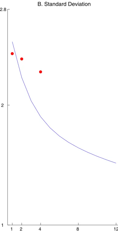
Figure 3 plots the mean and standard deviation of the ergodic distribution of yields at di erent maturities predicted by the model. These statistics are computed using a simulated sample of 5000 observations. The gure also reports data counterparts for these variables based on Treasury bill rates from 1960Q1 to 2001Q2. As we can see in panel A, the model
predicts an upward slopping term structure, as it is observed in the data. Notice, however, that the slope in the model is close to linear, while in the data it is concave. The model also correctly predicts an inverse relation between the standard deviation of interest rates and bond maturity (see panel B).
Consumption-based models of the term structure (see, for example, Backus et al., 1989, and den Haan, 1995) usually predict a downward-sloping term structure because long-term bonds have an insurance component: interest rates are low|or equivalently, bond prices are high|during recessions when consumption is low. Piazzesi and Schneider (2007) argue that if positive in ation surprises help forecast future decreases in consumption, then long-term bonds are risky in that their real payo is low when consumption is low. As a result, traders would demand a premium for holding long-term bonds and the term structure would be upward sloping. Rudebush and Swanson (2012) develop an asset-pricing model with pro-duction where a persistent technology shock induces this cross-correlation between in ation and consumption. In this model, the mechanism in Piazzesi and Schneider (2007) is ruled out by the assumption that in ation and consumption follow independent statistical processes. Instead, the bond premia that induces an upward sloping yield curve is primarily driven by preferences and ampli ed by the skewness of shocks. For example, the bond premia for the 2- and 8- period bonds are, respectively, -0.036 and -0.243 when innovations are drawn from normal distributions, but they are -0.039 and -0.257 when innovations are drawn from the estimated skew normal distributions.
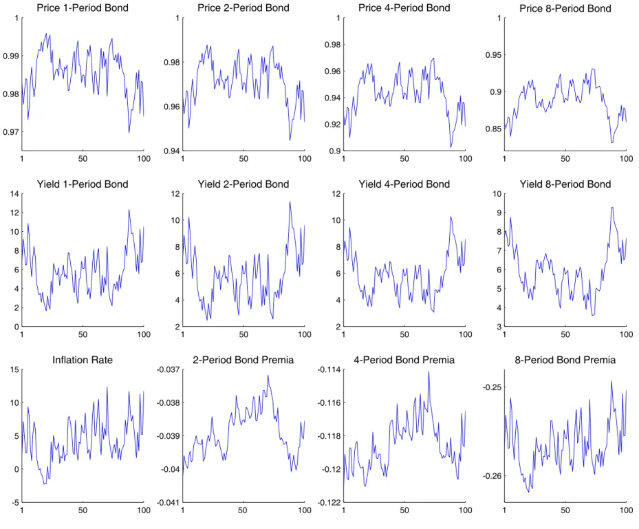
In order to examine the time-series behavior implied by the model, I simulated 5000 observations of bond prices, yields, and premia for di erent maturities. Figure 4 plots 100 observations of these variables. Considering rst the top and middle rows, note that bond prices are strongly correlated across maturities and that the price of long-term bonds is smoother than that of short-term bonds. The same holds true for yields. Also, note that there are large, occasional positive spikes in bond yields, which indicates that the unconditional distribution will likely be positively skewed. Finally, note that the arti cial data feature volatility clustering: there are periods where yields are quite volatile followed by periods where they are less so. (I will examine the latter two implications in detail below.)
Consider now the bottom row of gure 4, which plots observations of the bond premia implied by the model. Four conclusions follow. First, the magnitude of the bond premia is increasing with the maturity. Second, bond premia are relatively persistent, but persistence decreases with the maturity. For example, the rst-order autocorrelation of the 2-period bond premia is 0.94 while that of the 8-period bond is 0.62. Third, as in the case of yields, there are large, occasional spikes and volatility clustering in bond premia. Four, the bond premia is time-varying but clearly not as volatile as in the actual data.
4.2
Skewness
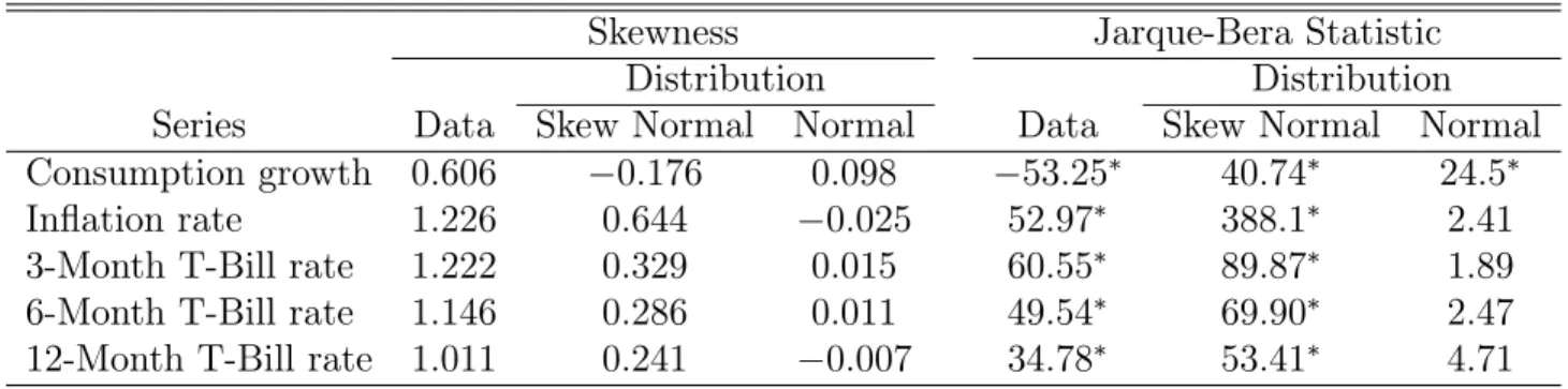
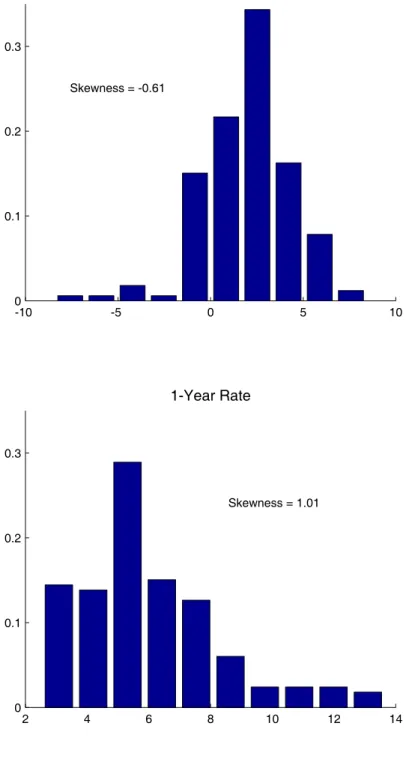
Skewness is a prominent feature of U.S. economic data. As we can see in gure 5, the unconditional distribution of in ation and of the three- and twelve-month Treasury-Bill rates are positively skewed, while that of consumption growth is negatively skewed. Estimates of the skewness are larger than +1 in the former cases and 0:6 in the latter case (see column 1 in table 2).
Column 4 of table 2 reports Jarque-Bera test statistics of the hypothesis that the data follow a normal distribution. This goodness-of- t test is based on sample estimates of the skewness and kurtosis, both of which are should be zero if the data are normal. Given the plots in gure 5, it is not surprising that test statistics are above the 5 percent critical value for all series and the hypotheses can be rejected.
Column 5 of table 2 reports Jarque-Bera test statistics computed from arti cial series gen-erated from the model with skew normal innovations. As for the actual data, the hypothesis of normality can be rejected at the 5 percent level in all cases. Moreover, the unconditional skewness predicted by the model (see column 2) is of the same sign as, although smaller magnitude than, the data. The observation that nancial variables, including bond yields, are skewed is one of the reasons Mandelbrot and Hudson (2004) propose relaxing the model-ing assumption of normality. These results show that adoptmodel-ing a more general and possibly asymmetric distribution function helps asset-pricing models better capture this feature of the data.
In contrast, note in column 6 that when Jarque-Bera tests are applied to arti cial series generated from the version of the model with normal innovations, the hypothesis that the data follow a normal distribution cannot be rejected at the 5 percent level for in ation and the nominal interest rates.10 The hypothesis can be rejected for consumption growth, but column 3 shows that its predicted skewness has sign opposite to that observed in the data (0:10 versus 0:60).
4.3
Volatility Clustering
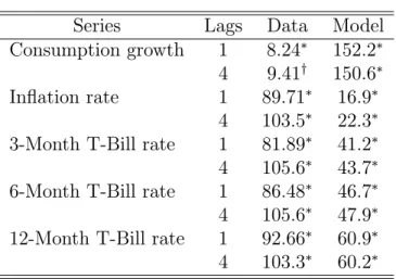
Another well-known feature of nancial and macroeconomic series is their time-varying volatility (see, for instance, the articles in Engle, 1995, and the literature on the Great Moderation). For the data used in this project, column 1 of table 3 reports Lagrange Multi-plier (LM) test statistics of the hypothesis of no conditional heteroskedasticity. Test statistics
10This result is not trivial because, in contrast to linear models which directly inherit their higher-order
properties from the distribution of the shocks, the nonlinearity of this model means that variables may be non-normal even if innovations are normal.
were calculated as the product of the number of observations and the uncentered R2 of the
OLS regression of the squared series on a constant and one (or four) of its lags. Under the null hypothesis, the statistic is distributed chi-squared with as many degrees of freedom as the number of lags in the regression. Note that the hypothesis can be rejected for all data series at the 5 percent signi cance level. The only exception is the rate of consumption growth when the regression includes four lags, where the hypothesis can be rejected at the 10 percent level instead.
Column 2 reports LM statistics from tests applied to arti cial data generated from the model. As for the actual data, the hypothesis of no conditional heteroskedasticity can be reject for all series at standard signi cance levels.11 The key point is that this result arises
despite the fact that shocks in the model are conditionally homoskedastic. Hence, this paper illustrates the quantitative importance of the non-linearity of the model as a mechanism that can endogenously generate predictable volatility clustering.12
Finally, let us refer back to our generic formulation of the policy function in (11) and notice that it includes (non-linear) quadratic and cubic terms in the state variables and a time-varying term in the variance. The latter term, that is (1=2)[fx (x; 0)]ja[(xt x)]a[ ][ ],
makes the policy function resemble the ARCH-M model use by Engle et al. (1987) to study the term structure, where the conditional variance directly a ects the mean. However, the key di erence is that while in the ARCH-M model the conditional variance is time-varying and its coe cient is constant, in this model the conditional variance is constant (by assumption) and its coe cient is time-varying because it is a linear function of the state variables.
5
Understanding Skewness Risk
Skewness risk arises in this model because, for given variances, traders face the possibility of extreme realizations from the upper tail of the distribution of in ation innovations and from the lower tail of the distribution of consumption innovations. The former reduce the real payo of the 1-period nominal bond and the real prices of longer-term nominal bonds. The latter increase marginal utility and the kernel used by traders to value nancial assets. Moreover, since the in ation and consumption processes are serially correlated, these e ects
11These results are based on a sample of 200 observations, but conclusions are robust to using instead
a sample of 5000 observations or other samples of 200 observations generated using di erent seeds for the random number generator.
12To my knowledge, the observation that nonlinear economic models can generate volatily clustering, even
when shocks are i:i:d: and parameters are time-invariant, was rst made by Granger and Machina (2006). Rudebusch and Swanson (2012) report results similar to the ones in this paper, but based on a medium-scale New Keynesian model with production.
are persistent. This section reports quantitative estimates of the contribution of skewness risk to the bond premia and of its e ect on bond prices in the pure exchange economy.
5.1
The Contribution of Skewness Risk to Bond Premia
As was pointed out above, in the special case where the innovation distribution is symmetric| and skewness is, therefore, zero|the bond premia depends only on the variance of the in-novations. In the more general case where the distribution is asymmetric, the bond premia depends on both the variance and skewness of the innovations. Examining the policy func-tions that solve the model and decompose the contribution of state variables and higher-order moments to the dynamics of each variable (see equation (11)) shows that they key di erence is the term (1=6)[f (x; 0)]j[ ][ ][ ], which is zero in the former case and non-zero in the
latter case.
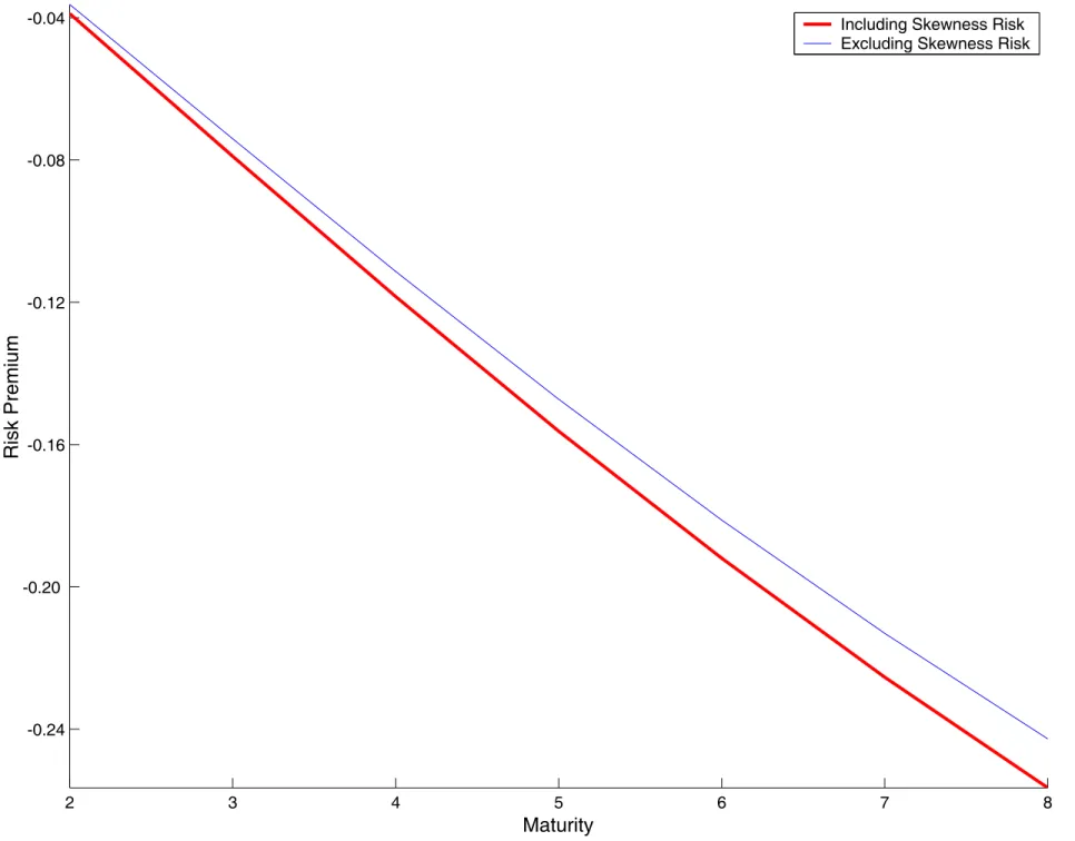
Figure 6 plots the bond premia predicted by the model with skew normal innovations (thick line) for maturities from 2 to 8 periods. As a benchmark, the gure also plots the premia predicted by a model where innovations are drawn from a normal distribution with the same variance as that of the skew normal distribution (thin line). All other parameters are the same in both models. This means that all terms in the policy functions, except for (1=6)[f (x; 0)]j[ ][ ][ ], are numerically identical in both models. In particular, the
variance risk is exactly the same. The gure is constructed using averages over 5000 simulated observations and the premia is annualized and expressed in percentage points.
Figure 6 shows that the model with asymmetric innovations delivers bond premia that are between ve and seven percent lower than in the model with normal innovations, and that this di erence increases with the bond maturity. From the discussion above, the distance between both lines is given by (1=6)[f (x; 0)]j[ ][ ][ ] in the policy function of the bond premia, which is negative in the former case and zero in the latter case.
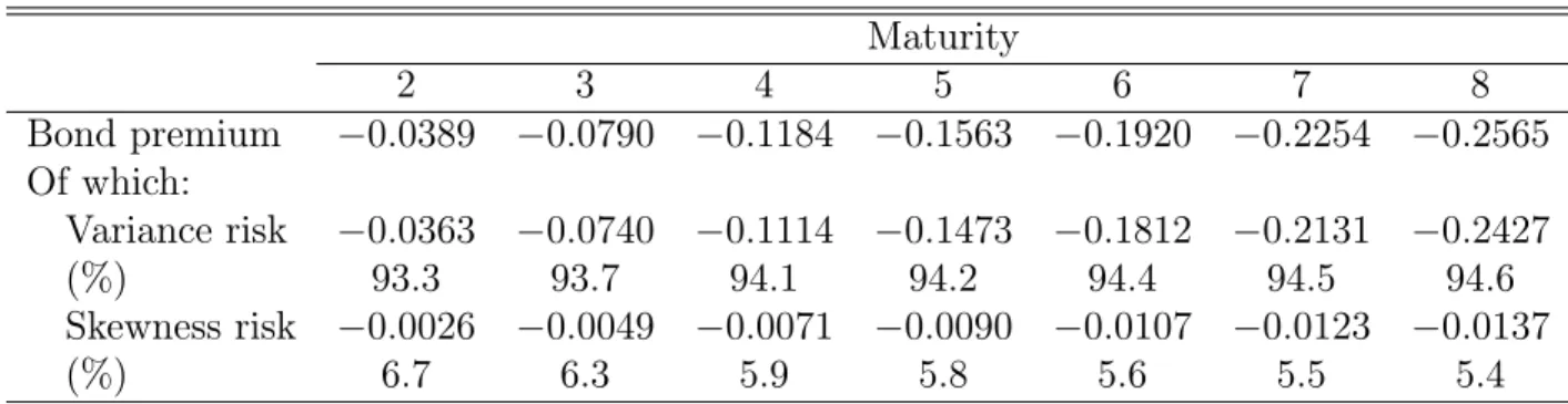
Table 4 decomposes the bond premia into the parts explained by the variance and by the skewness of the innovations at di erent maturities. This decomposition shows that variance risk accounts for 93 to 94 percent, and skewness risk accounts for 6 to 7 percent, of the bond premia depending on the maturity of the loan contract.
5.2
The E ect of Skewness Risk on Bond Prices
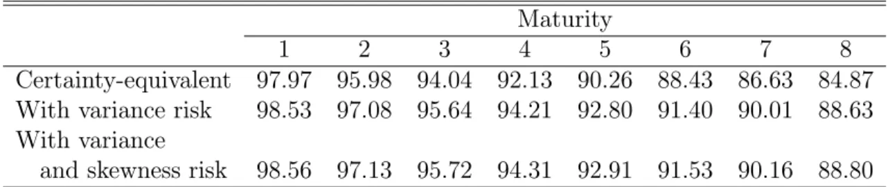
In order to quantify the e ect of skewness risk on bond prices, I compute the mean of the ergodic distribution of bond prices for the models with skew normal and with normal innovations. Table 5 reports the price (in cents) of a bond that pays one unit of currency at maturity, with the latter ranging from 1 to 8 periods. The rst row reports the
certainty-equivalent price. The second row reports the mean price when innovations are normally distributed and, hence, there is only variance risk. The third row reports the mean price when innovations are skew normal and there is both variance and skewness risk. As before, the variance of both distributions and all other parameters are the same for results in the second and third rows. Hence, all terms in the policy functions for bond prices, except for (1=6)[f (x; 0)]j[ ][ ][ ], and the variance risk are identical in both cases.
The di erence between the rst and second row in table 5 is just the di erence between the price of a bond in the certainty-equivalent economy and the price of a bond in an economy where symmetric shocks take place. As one would expected, risk-averse traders induce higher bond prices (and lower yields) in the latter case as they attempt to build up their precautionary savings. For example, variance risk increases the price of a 1-period bond by 0.56 cents and the price of an 8-period bond by 3.76 cents in the exchange economy.
The di erence between the second and third row in table 5 is the additional increase in bond prices associated with skewness risk. This additional price increase re ects the extra risk incurred when purchasing a nominal asset whose real payo /price may be unexpectedly reduced by a large positive in ation innovation drawn from the right tail of its positively-skewed distribution. The additional increase also re ects the extra risk that a large negative consumption innovation, drawn from the left tail of its negatively-skewed distribution, may unexpectedly increase the kernel used to value assets. Quantitatively, this skewness risk increases bond prices by 0.03 cents for the 1-period bond and 0.23 cents for the 8-period bond in the exchange economy. The reason skewness risk induces higher prices is the same the reason variance risk induces higher prices: traders faced with some risk attempt to save more and bid the price of nancial assets up. This risk is above and beyond the one associated with the variance of shocks but it a ects prices in the same direction as the latter.
Using the relation between yields and bond prices (6), it is possible to quantify the e ect of skewness risk on bond yields. As before, I compute the mean of the ergodic distribution of yields for the models with skew normal and with normal innovations. Provided that the variance of both distributions and all other parameters are the same, their di erence re ects skewness risk only. This calculation shows that skewness risk reduces the yield of the 1-period bond by 0:11 percentage points at the annual rate and of the 8-1-period bond by 0:09 percentage points.
In the nance literature, Kraus and Litzenberger (1976, 1983) examine versions of the capital asset pricing model (CAPM) that incorporates the e ect of skewness on valuations and nd that the coe cient of the market price of skewness is negative and statistically signi cant in Fama-MacBeth regressions. Harvey and Siddique (2000) focus on the condi-tional co-skewness with the aggregate market portfolio and argue that, since agents prefer
positively skewed portfolios, assets with negative co-skewness should have a higher expected return. This prediction is supported by industry portfolios that show a negative correlation between co-skewness and mean returns. Kapadia (2006) and Chang et al. (2012) nd that market skewness risk has a negative e ect on excess returns in a cross-section of stock returns and option data, respectively. For example, Chang et al. report market prices for skewness risk ranging between 3:72 percent and 5:16 percent per year. Since my approach and asset class are di erent theirs, quantitative estimates are not directly comparable. However, my nding that skewness risk reduces bond yields in the exchange economy is in qualitative agreement with this literature.
6
Dynamics
In this section, I use impulse-response analysis to study the e ects of in ation and consump-tion shocks on bond prices and yields. Since the model is non-linear, the e ects of a shock depend on its sign, size, and timing (see Gallant et al.,1993, and Koop et al., 1996). For this reason, I consider shocks of di erent sign and size, and assume that they occur when the sys-tem is at the stochastic steady state|i.e., when all variables are equal to the unconditional mean of their ergodic distribution. In particular, I study innovations in the 5th, 25th, 75th and 95th percentiles. Of course, the size (in absolute value) of innovation in the 5th and 95th (and in the 25th and 75th) percentile are not same because the distribution is asymmetric, but the point is that the likelihood of these two realizations is the same. The responses are reported in gures 7 and 8, with the vertical axis denoting percentage deviation from the stochastic steady state and the horizontal axis denoting quarters. Note that the yields in these gures are annualized.
Figure 7 plots the response of prices and yields to in ation shocks drawn from the skew normal distribution. Positive in ation shocks reduce bond prices and increase yields, but e ects are di erent across maturities. The e ect on prices increases monotonically with the maturity and eventually settles down so that, for example, the impact on 8- and 12-period bond prices is basically the same. The e ect on yields decreases monotonically with the maturity. For negative in ation shocks, the e ects are the opposite, that is, prices decrease and yields increase. However, as can be seen in gure 7, there is an asymmetry in that the positive shock in the 95th percentile delivers much larger responses than the equally likely negative shock in the 5th percentile. Interestingly, this asymmetry is reversed for the smaller shocks in the 25th and 75th percentiles.
The dynamic e ects of in ation shocks are driven by the persistence of in ation: a current, positive shock means higher in ation in future periods, and, as a result, traders
rationally expect a lower real payo for the 1-period bond and lower real bond prices for longer-term bonds in the future. When in ation is serially uncorrelated, a current shock has no e ect on prices or yields because the forecasts of future payo s and prices are unchanged. In this sense, what matters for bond prices and yields in this model is anticipated, rather than unanticipated, in ation.
Figure 8 plots the response to consumption shocks drawn from the skew normal distri-bution. Positive consumption shocks increase bond prices and reduce yields. The reason is simply that traders faced with an increased endowment would attempt to intertemporally smooth consumption by saving. Since this is not possible in the aggregate, bond prices must increase and yields decrease to induce traders to optimally consume the current output. The e ect on prices increases monotonically with the maturity, while that on yields is similar across maturities. As before, there is an asymmetry in the responses, with negative shocks at the 5th and 25th percentiles inducing larger e ects than the equally-likely, but positive, shocks at the 95th and 75th percentiles. As in the case of in ation, the dynamic e ects depend crucially on the persistence of the consumption process. When consumption is pos-itively autocorrelated, a current positive shock signals above-average consumption in future periods as well, and, so, the e ects described above take place in both the current and future periods. In contrast, when consumption is serially uncorrelated, the e ects take place in the current period only because, by construction, the economy will return to steady state next period.
Figure 9 plots the initial e ect of consumption and in ation shocks on the yields of bonds with di erent maturities. (By initial e ect, I mean the e ect of the shock in the period it takes place.) In panel A, the lines are almost horizontal because consumption shocks initially a ect all yields in a similar way regardless of the shock size. Thus, consumption shocks push the whole yield curve up or down, just like the level factor does in factor models of the term structure. Panel B shows that in ation shocks have a quantitatively larger e ect on short- than on long-term yields. As a result, in ation shocks change the slope of the yield curve. In this way, in ation acts like the slope factor in factor models. However, while statistical factors have no structural interpretation, in this model the level shifts and slope changes of the yield curve are empirically associated with observable macroeconomic variables, respectively aggregate consumption and in ation. Furthermore, in contrast to linear factor models, the e ects in this model are asymmetric. For example, the negative consumption shock at the 5th percentile induces a larger upward shift of the yield curve e ects than the equally-likely, but positive, shock at the 95th percentile.
7
Conclusions
This paper examines the implications of skewness risk for bond pricing and returns in a pure exchange economy. For a given variance, the possibility of extreme realizations from the long tail of the in ation and consumption distributions a ects prices, returns and the pricing kernel used by traders to evaluate payo s. Quantitative magnitudes of these e ects are computed based on parameters estimated from U.S. data. These estimates show that in ation innovations are drawn from a positively skewed distribution, that consumption innovations are drawn from a negatively skewed distribution, and that the hypotheses that they are drawn from normal distributions are rejected by the data.
Results reported in this paper are relevant for three streams of the literature. First, for the growing literature on consumption disasters, this paper shows that even outside disaster episodes, agents face the possibility of substantial consumption decreases primarily associated with recessions, as well as the possibility of positive in ation surprises. While the magnitude of these consumption decreases is not as dramatic as disasters, they are shown to have non-negligible implications for asset pricing. Second, for the nance literature on the role of higher-order moments on valuations, this paper quantitatively shows that in an exchange economy, most of the bond premia is driven by variance risk but that skewness risk nonetheless accounts for 6 to 7 percent of the premia depending on the bond maturity. Skewness risk also has non-negligible e ects on bond prices and yields which are qualitatively similar to those reported for cross-sections of stock return and option prices. Finally, for the statistical literature on factor models of the term structure, this paper presents a model whose state variables (i.e., aggregate consumption and in ation) behave empirically like \slope" and \level" factors but have a clear macroeconomic interpretation.
In interpreting these results it is important to consider the following caveats. Needless to say, quantitative estimates depend on the model speci cation. The use of an exchange economy was motivated by the desired to examine skewness risk in a simple and transparent environment, but in ongoing work I consider production economies with a larger asset menu. Also, it is possible that results reported here under-estimate the e ects of skewness risk because, as seen in table 2, the model does not completely match the unconditional skew-ness of yields and the e ects of in ation skewskew-ness risks are mitigated by the assumption of completely exible good prices. Finally, nancial-market imperfections may be potentially important and key to model the mechanism outlined in Hicks (1939) whereby long-term bonds are somehow \less liquid" than short-term bonds.
Table 1. Parameter Estimates
Consumption Measure Nondurables Nondurables Parameter and Services Only Preferences Discount factor 0:9904 0:9597 (0:0147) (0:0882) Intertemporal elasticity 0:1632 0:1862 (0:1404) (0:1573) Risk aversion 49:774y 49:562 (38:010) (15:377) In ation Steady state 1:0110 1:0110 (0:0013) (0:0013) Autoregressive coe cient 0:5663 0:5587
(0:0422) (0:0462) Correlation parameter 0:9998 0:9998 (0:0112) (0:0110) Scale parameter 0:0113 0:0115 (0:0007) (0:0009) Consumption
Autoregressive coe cient 0:9705 0:9703 (0:0523) (0:0575) Correlation parameter 0:9977 0:9977 (0:0456) (0:0326) Scale parameter 0:0104 0:0138
(0:0020) (0:0017)
Note: The gures in parenthesis are asymptotic standard errors. The superscripts andy de-note statistical signi cance at the 5 and 10 percent signi cance levels respectively. Estimates of the correlation and scale parameters imply that the standard deviation and skewness of the in ation innovations are 0:007 and 0:99, respectively, while those of the consumption innovations are 0:006 and 0:97, respectively.
Table 2. Skewness and Jarque-Bera Tests
Skewness Jarque-Bera Statistic Distribution Distribution Series Data Skew Normal Normal Data Skew Normal Normal Consumption growth 0:606 0:176 0:098 53:25 40:74 24:5 In ation rate 1:226 0:644 0:025 52:97 388:1 2:41 3-Month T-Bill rate 1:222 0:329 0:015 60:55 89:87 1:89 6-Month T-Bill rate 1:146 0:286 0:011 49:54 69:90 2:47 12-Month T-Bill rate 1:011 0:241 0:007 34:78 53:41 4:71
Note: Under the null hypothesis of normality, the Jarque-Bera statistic follows a chi-squared distribution with two degrees of freedom. The sample size of the arti cial data is 5000 observations. The superscript denotes the rejection of the hypothesis at the 5 percent signi cance level.
Table 3. ARCH Tests
Series Lags Data Model Consumption growth 1 8:24 152:2
4 9:41y 150:6
In ation rate 1 89:71 16:9 4 103:5 22:3 3-Month T-Bill rate 1 81:89 41:2 4 105:6 43:7 6-Month T-Bill rate 1 86:48 46:7 4 105:6 47:9 12-Month T-Bill rate 1 92:66 60:9 4 103:3 60:2
Note: Under the null hypothesis of no conditional heteroskedasticity, the statistic follows a Chi-squared distribution with as many degrees of freedom as the number of lags in the regression. The sample size of the arti cial data is 200 observations. The superscripts andy respectively denote the rejection of the hypothesis at the 5 and 10 percent signi cance levels.
Table 4. Decomposition of the Bond Premia Maturity 2 3 4 5 6 7 8 Bond premium 0:0389 0:0790 0:1184 0:1563 0:1920 0:2254 0:2565 Of which: Variance risk 0:0363 0:0740 0:1114 0:1473 0:1812 0:2131 0:2427 (%) 93:3 93:7 94:1 94:2 94:4 94:5 94:6 Skewness risk 0:0026 0:0049 0:0071 0:0090 0:0107 0:0123 0:0137 (%) 6:7 6:3 5:9 5:8 5:6 5:5 5:4
Note: The premia are expressed at an annual rate and are computed as the sample average of 5000 simulated observations. The gures for the variance risk include the part due to time-varying volatility.
Table 5. Bond Prices
Maturity
1 2 3 4 5 6 7 8
Certainty-equivalent 97:97 95:98 94:04 92:13 90:26 88:43 86:63 84:87 With variance risk 98:53 97:08 95:64 94:21 92:80 91:40 90:01 88:63 With variance
and skewness risk 98:56 97:13 95:72 94:31 92:91 91:53 90:16 88:80
References
[1] Ang, A., Piazzesi, M., 2003. A No-Arbitrage Vector Autoregression of Term Structure Dynamics with Macroeconomic and Latent Variables. Journal of Monetary Economics 50, pp. 723-744.
[2] Bansal, R., Coleman, J. W., 1996. A Monetary Explanation of the Equity Premium, Term Premium, and Risk-Free Rate Puzzles. Journal of Political Economy 104, pp. 1135-1171
[3] Backus, D. K., Gregory, A., Zin, S. E., 1989. Risk Premiums in the Term Structure: Evidence from Arti cial Economies. Journal of Monetary Economics 24, pp. 371-399.
[4] Barro, R. J., 2006. Rare Disasters and Asset Markets in the Twentieth Century. Quar-terly Journal of Economics 121, pp. 823-866.
[5] Barro, R. J., 2009. Rare Disasters, Asset Prices, and Welfare Costs. American Economic Review 99, pp. 243-264.
[6] Barro, R. J., Nakamura, E., Steinsson, J., Ursua, J., 2010. Crises and Recoveries in an Empirical Model of Consumption Disasters. Harvard University, Mimeo.
[7] Brunnermeier, M. K., Gollier, C., Parker, J. A., 2007. Optimal Beliefs, Asset Prices, and the Preference for Skewed Returns. American Economic Review 97, pp. 159-165.
[8] Caldera, D., Fernandez-Villaverde, J., Rubio-Ram rez, J. F., 2009. Computing DSGE Models with Recursive Preferences. Review of Economic Dynamics, forthcoming.
[9] Campbell, J. Y., 1986. Bond and Stock Returns in a Simple Exchange Model. Quarterly Journal of Economics 101, pp. 785-803.
[10] Campbell, J. Y., 1996. Understanding Risk and Return. Journal of Political Economy 104, pp. 298-345.
[11] Chang, B. Y., Christo ersen, P., Jacobs, K., 2012. Market Skewness Risk and the Cross-Section of Stock Returns. Journal of Financial Economics, forthcoming.
[12] Cochrane, J. H., Piazzesi, M., 2005. Bond Risk Premia. American Economic Review 95, pp. 138-160.
[13] Culbertson, J. M., 1957. The Term Structure of Interest Rates. Quarterly Journal of Economics 71, pp. 485-517.
[14] den Haan, W., 1995. The Term Structure of Interest Rates in Real and Monetary Economies. Journal of Economic Dynamics and Control 19, pp. 909-940.
[15] Diebold, F. X., Rudebusch, G., Aruoba, B., 2006. The Macroeconomy and the Yield Curve: A Dynamic Latent Factor Approach. Journal of Econometrics 131, pp. 309-338.
[16] Doh, T., 2008. Long Run Risks in the Term Structure of Interest Rates: Estimation. Federal Reserve Bank of Kansas City Working Paper 08-11.
[17] Du e, D., Singleton, K. J., 1993. Simulated Moments Estimation of Markov Models of Asset Prices. Econometrica 61, pp. 929-952.
[18] Engle, R. F., 1995. ARCH: Selected Readings, Oxford: Oxford University Press.
[19] Engle, R. F., Lilien, D. M., Robins., R. P., 1987. Estimating Time Varying Risk Premia in the Term Structure: The ARCH-M Model. Econometrica 55, pp. 391-407.
[20] Epstein, L., Zin, S., 1989. Substitution, Risk Aversion, and the Temporal Behavior of Consumption and Asset Returns: A Theoretical Framework. Econometrica 57, pp. 937-969.
[21] Epstein, L., Zin, S., 1991. Substitution, Risk Aversion, and the Temporal Behavior of Consumption and Asset Returns. Journal of Political Economiy 99, pp. 263-286.
[22] Gallant, A. R., Rossi, P. E., Tauchen, G., 1993. Nonlinear Dynamic Structures. Econo-metrica 61, pp. 871-908.
[23] Golec, J, Tamarkin, M., 1998. Bettors Love Skewness, Nor Risk, at the Horse Track. Journal of Political Economy 106, pp. 205-225.
[24] Granger, C., Machina, M., 2006. Structural Attribution of Observed Volatility Cluster-ing. Journal of Econometrics 135, pp. 15{29.
[25] Gregory, A., Voss, G. M., 1991, The Term Structure of Interest Rates: Departures from Time-Separable Expected Utility. Canadian Journal of Economics 24, pp. 923-939.
[26] Hall, R. E., 1988. Intertemporal Substitution in Consumption. Journal of Political Econ-omy 96, pp. 339-357.
[27] Hansen, L. P., Singleton, K., 1982. Generalized Instrumental Variable Estimation of Nonlinear Rational Expectations Models. Econometrica 50, pp. 1269-1286.
[28] Hansen, L. P., Singleton, K., 1983. Stochastic Consumption, Risk Aversion, and the Temporal Behavior of Asset Returns. Journal of Political Economy 91, pp. 249-265.
[29] Harvey, C. R., Siddique, A., 2000. Conditional Skewness and Asset Pricing Tests. Jour-nal of Finance 55, pp. 1263-1295.
[30] Hicks, J., 1939. Value and Capital, Oxford: Clarendon Press.
[31] Jermann, U. J., 1998. Asset Pricing in Production Economies. Journal of Monetary Economics 41, pp. 257-275.
[32] Jin, H., Judd, K. L., 2002. Perturbation methods for general dynamic stochastic models. Hoover Institution, Mimeo.
[33] Kapadia, N., 2006, The Next Microsoft? Skewness, Idyosincratic Volatility, and Ex-pected Returns. Rice University, Mimeo.
[34] Kim. J., Kim, S., Schaumburg E., Sims, C., 2008. Calculating and Using Second-Order Accurate Solutions of Discrete-Time Dynamic Equilibrium Models. Journal of Economic Dynamics and Control 32, pp. 3397-3414.
[35] Koop, G., Pesaran, M. H., Potter, S., 1996. Impulse Response Analysis in Nonlinear Multivariate Models. Journal of Econometrics 74, pp. 119-147.
[36] Kraus, A., Litzenberger, R. H., 1976. Skewness Preference and the Valuation of Risky Assets. Journal of Finance 31, pp. 1085-1100.
[37] Kraus, A., Litzenberger, R. H., 1976. On the Distributional Conditions for a Consump-tion Oriented Three Moment CAPM. Journal of Finance 38, pp. 1381-1391.
[38] Le, A., Singleton, K. J., 2010. An Equilibrium Term Structure Model with Recursive Preferences. American Economic Review 100, pp. 1-5.
[39] Lee, B.-S., Ingram, B. F., 1991. Simulation Estimation of Time-Series Models. Journal of Econometrics 47, pp. 195-205.
[40] Ljungqvist, L., Sargent, T., 2004. Recursive Macroeconomic Theory, Cambridge: MIT Press.
[41] Mandelbrot, B., Hudson, R., 2004. The (mis)Behavior of Markets, New York: Basic Books.