To cite this version :
Lecointe, Maxime and Ponzoni Carvalho
Chanel, Caroline and Defay, François
Backstepping control law
application to path tracking with an indoor quadrotor.
(2015)
In: Proceedings of European Aerospace Guidance Navigation and
Control Conference (EuroGNC), 13 April 2015 - 15 April 2015
(Toulouse, France).
O
pen
A
rchive
T
OULOUSE
A
rchive
O
uverte (
OATAO
)
OATAO is an open access repository that collects the work of Toulouse researchers and
makes it freely available over the web where possible.
This is an author-deposited version published in :
http://oatao.univ-toulouse.fr/
Eprints ID : 14669
Any correspondance concerning this service should be sent to the repository
administrator:
[email protected]
tracking with an indoor quadrotor
Maxime Lecointe, Francois Defay, and Caroline P. Carvalho Chanel
Abstract
This paper presents an application of the backstepping control to a path tracking mission using an indoor quadrotor. This study case starts on modeling the quadrotor dynamics in order to design a backstepping control which we applied directly to the Lagrangian dynamic equations. The backstepping control is chosen due to its ap-plicability to this class of nonlinear and under-actuate system. To test the designed control law, a complete quadrotor model identification was performed, using a mo-tion capture system. The procedure used to obtain a good model approximamo-tion is presented. Experimental results illustrate the validity of the designed control law, including rich simulations and real indoor flight tests.
1 Introduction
Remotely Piloted Aircraft Systems (RPAS) have been used in many civil or mili-tary applications. One can cite missions like : surveillance, search and rescue, target tracking, cartography, etc. To well fulfill the mission, it is mandatory the RPAS would be able to move in a constraint flight space following some complex path. The quality of the movement depends on a lot of parameters and functions. One can cite : the control law used to stabilize and to move the RPAS to some position; the navigation component used to track the state of the system; the guidance com-ponent used to infer input references to the control depending on the environment constraints and on the motion planning; the mission planning which defines the
or-M. Lecointe · F. Defay · C. P. Carvalho Chanel Universit´e de Toulouse
ISAE-SUPAERO Institut Sup´erieur de l’A´eronautque et le l’Espace DMIA - Department of mathematics, computer science and automatic control 10 av. Edouard Belin - BP 54032 - 31055 TOULOUSE Cedex 4 - FRANCE
e-mail: [email protected], [email protected], [email protected]
der of movements to reach the mission goal, and which quality and efficiency is answerable to how good the GNC (guidance, navigation and control) components work.
The attitude control and modeling of a quadrotor is studied since many years [1],[7], one can notice that full control is not currently used on quadrotor applica-tion. Some papers, as [3] deals with, but the applicative case on real testbed is not a lot published. Today, the classical approach (cascade loop for attitude, navigation), as introduced by Hamel et al. [7], supposes that roll, pitch, yaw axes are not cou-pled. Backstepping approach is used since a long time for quadrotor in simulation [2],[4],[9] but few papers deals on the applicative case, which is the aim of this paper.
In this paper, the main interest is to provide an easy way to track a path for a quadrotor for indoor flight purpose. For this application, the classical PID approach for attitude stabilization is chosen because of its good performance, stability and robustness. Trajectory or path tracking is more and more studied since quadrotor’s open source projects and friendly testbed are available. Some control laws have al-ready been used [11], but few of them present experimental results [13]. Backstep-ping approach was chosen in this paper using the Lagrangian dynamics equations [5]. This paper presents a complete applicative case study of path tracking on a real testbed, using a complete quadrotor model in Simulink to tune the control param-eters. The final interest on this UAV framework is to provide a stabilized UAV in order to achieve complex missions as target detection and formation flying in con-straint environments.
The paper is organized as follows: Section 2 presents the experimental frame-work, the AR.drone’s model and the attitude stabilization. In Section 3, the back-stepping applicative case for path tracking is presented. Finally, Section 4 shows some experimental results to demonstrate the interest of the approach.
2 Quadrotor dynamics
2.1 Testbed framework
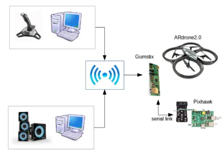
At ISAE-SUPAERO Institute, a complete framework has been developed to study UAV and robots applications. For students’s works and research on guidance and planning, the AR.drone quadrotor developed by the Parrot Society is chosen. There-fore, only the mechanical basis, motors and propellers was conserved. All the em-bedded electronics used to control the UAV was changed by a Pixhawk device [10] for the attitude stabilization. There is an other electronic device, a Gumstix board, carried with a wifi key which is used to deploy the embedded robotic architecture composed of all necessary components, as for instance, the state estimation com-ponent. The high level Gumstix device is connected with the Pixhawk device by a serial connection, and with the ground station by a wifi connection. In the ground
Fig. 1 Framework environment description.
station, the operator can chose between control himself with a joystick device the quadrotor or control the quadrotor using the automatic path generation and the back-stepping control law.
The figure 1 shows a description of the test environment. The flight area, about 50m2, is equipped with an ’OptiTrack’ motion capture system. It allows us to decou-ple the indoor localization problem and the control law design problem. The motion capture system is able to send directly to the Gumstix board the local position and speed with a frequency highest than 100Hz. This information is treated by a special designed component on the robotic real time architecture.
The robotic real time architecture used is the Orocos Toolchain [6]. Orocos is based on modular and run-time configurable software components. In Orocos each component has an standard interface based on input and output ports for the data flow, properties and services. In our application case, communication with the mo-tion capture system, state estimamo-tion and control are encapsulate in Orocos
compo-Fig. 2 Orocos components (in gray color), Matlab (in yellow), transmission blocks (in blue) schema.
nents and connected between them. Orocos guarantee real time and safety commu-nications between components.
The ground station is a computer carried with the joystick device and where the Matlab Real Time Windows Target application runs. Hence the operator can chose to control manually or automatically the quadrotor. The designed control law and path generation are computed in real time on Matlab with a frequency of 100Hz. So all, the control laws are discretized by automatic code generation tools of Mat-lab/Simulink. Matalb/Simulink performs the human-machine interface and allows to directly obtain the results of the new control laws.
In the Figure 2 the Orocos components schema is shown. Note that Matlab real time target is used to read (UDP socket) the information coming from the state estimation component turning on the Gumstix board, and to send the computed command (UDP socket) to the control component running on the Gumstix board. For real flight tests, it was necessary to sample the control with the same period used by the communication system (send/reception of UDP pack). It is interesting to observe that the frequency used for communication is enough to guarantee no latency or excessive delays.
2.2 Quadrotor model
A quadrotor is a rotary wing aircraft composed by four rotors to its lift. These four rotors are generally placed on the cross extremities of the rigid structure of the aircraft. In the center of the rigid structure the embedded electronic for the control and battery are placed. To avoid the aircraft turns over itself, two rotors usually turn in clockwise sense and the others two rotors in counter-clockwise sense. Hence, to control the movement of the aircraft, it is usual to place each couple of rotors turning in the same sense in opposite way on the rigid cross structure. The Figure 3(b) illustrate this principle.
(a) Local and inertial frames for the ARdrone 2.0 structure used for this study.
(b) Lift forces schema.
The generalize configuration of the quadrotor is q = (x, y, z, ϕ, θ , ψ), where (x, y, z) represents the relative position of the center of mass of the quadrotor, with re-spect to a local frame, and (φ , θ , ψ) are the three Euler angles representing the orien-tation of the rotorcraft, with respect to a local frame, namely yaw, pitch and roll. The translational and rotational variables are respectively defined as ξ = (x, y, z)T ∈ R3 and η = (ϕ, θ , ψ)T ∈ R3.
The total mass of the quadrotor (m) corresponds to the sum of this rigid cross structure (mc), the mass of the four rotors (mi), considered as identical, and the mass of the embedded electronic and battery (mb),
m= m1+ m2+ m3+ m4+ mc+ mb (1) Considering that the quadrotor is perfectly symmetric, ignoring the Coriolis (cen-tripetal) forces, and finally doing hypothesis that the effective inertia is constant, the inertia matrix J can be written as :
J= Ix 0 0 0 Iy 0 0 0 Iz (2)
where, Ixrepresents the inertia on the −→v axis which goes throw in the cross’ center between the front and rear rotors, Iy represents the inertia over the −→u axis which goes throw the cross’ center between the right and left rotors, and finally Iz rep-resents the inertia over the −→w axis, perpendicular to the v and u plan (see Figure 2.2).
Note that only these physical parameters m and J are used to pose and solve mechanical equations of our control system. In this paper, this control scheme is dedicated for indoor navigation and planning study, one can assume that the relative ground speed is low, so this simplification is justified. We empathize that the simple mechanical model used in this study does not implicate our approach as it will be seen in the next sections.
The simple mechanical model equation can be written as:
m ¨ξ + 0 0 −mg = Fd (3)
and, considering that the coriolis term is neglicted, the rotational subsystem is given by:
J ¨η = τ (4)
where Fdand τ represents respectively the thrust force and the total torque. In order to better design the control law to path tracking purpose, the aerody-namic forces and torques involved in our application have to be identified in order to find the link between these forces and the speed rotation of rotors.
Aerodynamic forces
The principle of the movement is simple, for example: pitch movement is obtained by increasing (resp. reducing) the speed of the rear motors while reducing, (resp. increasing) the speed motor of the front motors. The same idea can be used to un-derstand the roll movement. The yaw one is obtained by increasing (resp. reducing) the rear and front speed motors as the same time as decreasing (resp. increasing) right and left speed motors.
More precisely, the aerodynamic forces can be divided into two projected forces related to two axes. First, the drag force is parallel to the rotation plan of rotors, i.e to the −→v and −→u axis. It corresponds to the drag drill when in quadrotor is in air, due to the mass air acceleration against to the blades of the rotors.
fdi = kdω
2
i (5)
where fdi is the drag force of each rotor i ,kdthe drag coefficient, and withe rotation
speed of each rotor i.
Secondly, the lift force can be observed which is conduct in the perpendicular axis with respect to the rotor rotation plan. This force is responsible for the weight compensation and its enable the quadrotor to remain in air.
fi= kωωi2 (6) where , firepresents the lift force of each rotor i, kwrepresents the thrust coefficient, and withe speed rotation of the rotor i.
Once the aerodynamic forces induced by the propellers are defined, the active torques responsible to the movement of the quadrotor can be deduced.
Movements
The upward and downward movement is the translational movement with respect to the inertial frame of the quadrotor −→w. There is a nominal speed rotation of blades w0 where the lift produced by the propellers compensated the weight of the quadrotor. In this case if the rotation speed if smaller than w0the quadrotor tends to downward, and on the contrary, it tends to upward. This movement is then related to the lift force u, composed by the sum of all rotor’s lift forces:
u= kω 4
∑
i=1
ωi2 (7)
Note that, the thrust force Fdcan be now write as a function of the lift force:
Fd= Tr/bT 0 0 u = u
sin ϕ sin ψ + cos φ sin θ cos ψ − sin ϕ cos ψ + cos ϕ sin θ sin ψ
cos ϕ cos θ
where Tr/bis a rotation matrix between the local frame and the inertial frame [12] (see Fig. 3(a)), given by:
Tr/b= 1 0 0 0 cos π sin π 0 sin π cos π
cos ψ cos θ sin ψ cos θ − sin ψ
cos ψ sin θ sin ϕ − sin ψ cos ϕ sin ψ sin θ sin ϕ + cos ψ cos ϕ cos θ sin ϕ cos ψ sin θ cos ϕ + sin ψ sin ϕ sin ψ sin θ cos ϕ − cos ψ sin ϕ cos θ cos ϕ
(9)
The roll movement (τφ) is the rotation with respect to the −→u axis in the inertial frame resulting from the torque generated by the difference between lift forces of the left and right rotors. For instance, the movement to the left is consequence of the reduction in rotation speed of the rotors 2 and 3 (see Fig. 3(b)) of ∆ ω, and inversely the growth of the rotation speed of the rotors 1 and 4, with the same ∆ ω. In the same way, the pitch movement (τϕ) is the rotation with respect to the −→v axis in the inertial frame. Finally, the yaw movement (τψ) is the rotation with respect to the −→w axis in the inertial frame. Hence, the roll, pitch and yaw torques can be written as:
τϕ= ka( f1− f2− f3+ f4) (10) τθ = ka( f1+ f2− f3− f4) (11) τψ= kc( f1− f2+ f3− f4) (12) where ka= l/
√
2, with l the distance between the center of rotor i and the center of the rigid cross structure, and kcis the report between drag and thrust coefficients, i.e. kc= kd/kω.
Now, once can define the control inputs (u, τT)T of our system in terms of forces of the four rotors by the relation:
u τϕ τθ τψ = 1 1 1 1 ka−ka−ka ka ka ka −ka−ka kc−kc kc −kc | {z } M f1 f2 f3 f4 | {z } f = M f (13)
In summary, the coupled Lagrangian form of the dynamics is given as:
m ¨ξ = u
sin ϕ sin ψ + cos φ sin θ cos ψ − sin ϕ cos ψ + cos ϕ sin θ sin ψ
cos ϕ cos θ − 0 0 −mg (14) J ¨η = τϕ τθ τψ (15)
where u ∈ R and τ ∈ R3are the control inputs.
Note that this system is an under-actuated system with six outputs and four in-puts. Therefore this system is also a nonlinear system. In this papers, and for low dynamics, the classical reproach with cascade loop for attitude and navigation con-trol laws is chosen.
2.3 AR.drone attitude control
In order to achieve navigation, the attitude loop has to be tuned with low overshoot and good response time (approximatively 0.5s). On the experimental framework, the Pixhawk card and the last firmware are used. In this context, the proposed PID controller for attitude loop is used inside the Pixhawk card. Figure 4 presents the simplified blocks of the cascade loop. A PID (Cpos(z) in Fig. 4) is used for the each rotational angular velocity ( ˙θ , ˙φ , ˙ψ ) and a PID (Cspeed(z) in Fig. 4) is used for each angular position (θ , φ , ψ).
Fig. 4 Embedded Pixhawk attitude control.
The initial parameters for the PID regulators that are given in the last firmware of Pixhawk card are not well tuned for our application’s need. In order to take benefit of this framework, the model has been identified collecting flight test data. So, we have obtained inertial, mass and aerodynamic coefficients for the AR.dorne, with Pixhawk card, gumstix board and USB wifi key. They are explicit shown bellow : Ix= Iy= 0.0039Kg.m2 Iz= 0.0077Kg.m2 m= 0.38Kg kω= 9.17 · 10−6N/rad.s−1 kd= 1.37 · 10−6N.m/rad.s−1 ka= 0.13m kc= 0.15m
The simulation was performed with a complete Matlab/Simulink model using the 6DOF block and assuming a constant inertia. Aerodynamic drag forcse induced by the movement are token into account and have been identified for low speed movements. The complete model includes coupling forces, gyroscopic effects but is not detailed in this paper.
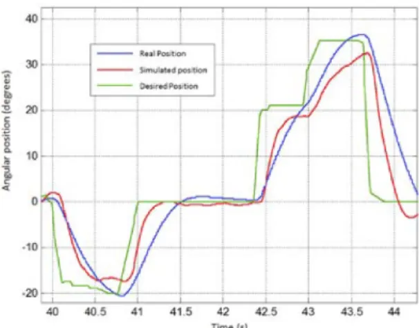
Figure 5 shows a comparison between the experimental results and the simulated results with manual control with joystick. The joystick inputs are recorded and in-jected in the Simulink files. The comparison between both models is not perfect but is quite good to improve the tunning of the gains. To obtain this results, the new regulator parameters used in the Pixhawk card are now:
Fig. 5 Pitch attitude comparison between flight test and simulation.
roll, pitch attitude : kp= 8 ki= 0.1 kd= 0 roll, pitch rate : kp= 0.13 ki= 0 kd= 0 yaw attitude: kp= 0.2 ki= 0.15 kd= 0 yaw rate: kp= 0.3 ki= 0.2 kd= 0
(16)
The controllers outputs are mixed and multiplied by a scale factor inside the Pixhawk to deliver the rotational speed desired for each brushless motors. One can notice that, the second order equivalent model between the angular position and the command input has an overshoot of 5% and a response time around 0.6 sec. This attitude control is enough robust and smooth to be included in the navigation loop which is developed with backstepping in the next section.
3 Backstepping control
The backstepping method was developed in 90’s by [8] in the aim to conceive meth-ods for stabilizing a particular class of dynamic nonlinear systems. The principal idea is the system can be decomposed in subsystems that are themselves concen-trated around an irreducible subsystem that can be stabilized. Hence, the engineer can start the control process on the level of the stable irreducible subsystem and comes back with the control to stabilize the outer subsystems.The process is finish when the outer control feedback is reached. The backstepping approach propose a recursive approach in order to stabilize the origin of a system in strict feedback control.
Usually, people use to design the backstepping control based on state variable form, which introduces unnecessary complications, as highlighted by [4]. In the same way that [4], we have chosen to apply backstepping control directly to the Lagrangian dynamics equations.
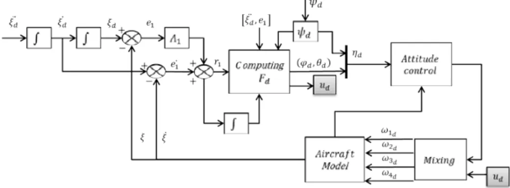
Fig. 6 Backstepping control law schema block.
In the next paragraph, the backstepping control designed is presneted, where the aim is to track a path defined as position, speed and acceleration smooth trajectories.
Position feedback control
The Figure 6 presentes the schema block used to design the backstepping control law. Next, necessary calculations to better understand this schema are detailled.
The first step to designing control law is determine the position error , and speed error dynamics. In this way, the position track error e1(t) and speed track error ˙e1(t) of the subsystem are described:
e1= ξd− ξ (17) ˙
e1= vd− v (18) where, ξdand vdare respectively the desired positions and desired speed.
One can define also, a sliding mode error r1(t) [4] , that aggregate position error and speed error as a linear combination, also namely filtered error:
r1= ˙e1+ Λ1e1 (19) where, Λ1is a diagonal positive definite constant parameters matrix. It can be show that, as the Λ matrix is diagonal with positive entries (so, a stable system), the error e1is bounded as long as the filtered error r1remains bounded [4].
Note that, the objective is clearly to design a controller that forces the system to get r1small. The parameter Λ1is so selected for a desired sliding mode response as e1(t) = e1(0)e−Λ1t, for which the point ˙e1+ Λ1e1= 0 defines a stable sliding mode.
To reveal the filtered error in the dynamics equation, Eq. 19 is multiplied by the mass m of the system and afterwards derivate on time:
m˙r1= m ¨e1+ mΛ ˙e1 (20) m˙r1= m ¨ξd− m ¨ξ + mΛ1(r1− Λ1e1) (21)
m˙r1= m ¨ξd− Fd− 0 0 −mg + mΛ1r1− mΛ12e1 (22)
where, Fd is given by equation 8. Rewriting Eq. 22 with a proportional Kr1 and an
integral Ki1 definite positive matrix gains, we have:
Fd= m ¨ξd+ 0 0 −mg − mΛ12e1+ Kr1r1+ Ki1 Z t 0 r1dt (23)
Note that, on can define the close-loop position error dynamics as:
−m˙r1+ mΛ1r1= Kr1r1+ Ki1 Z t 0 r1dt (24) m˙r1= mΛ1r1− Kr1r1− Ki1 Z t 0 r1dt (25) m˙r1= −(Kr1− mΛ1)r1− Ki1 Z t 0 r1dt (26)
Fd now help us to determine the control inputs u and τ in the design control procedure. Is this relation that shows the principal interest of the Lagrangian form to backstepping procedure.
In this sense, one can impose the yaw value ψd, and explicitly determine ud, θd and ϕd from Fd (see Eq. 8). It can be obtained noting that ||Fd|| = u and writing kcψ= cos ψdand ksψ= sin ψd, as:
Fd= u
sin ϕ sin ψ + cos φ sin θ cos ψ − sin ϕ cos ψ + cos ϕ sin θ sin ψ
cos ϕ cos θ (27) Fd= ||Fd|| ksψ kcψ 0 −kcψ ksψ 0 0 0 1 | {z } Cψ sin ϕd cos ϕdsin θd cos ϕdcos θd = ||Fd|| Cψ sin ϕd cos ϕdsin θd cos ϕdcos θd (28) resulting in : sin ϕd cos ϕdsin θd cos ϕdcos θd = C−1ψ Fd ||Fd|| = fd1 fd2 fd3 (29)
giving that Cψis a define positive rotation matrix.
As ψdis imposed, what allow us to always define Cψmatrix, we have (ϕd, θd, ud)T computed by:
ud= ||Fd||, ϕd= arcsin fd1, θd= arctan
fd2 fd3
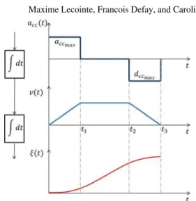
Fig. 7 Acceleration, speed and position profiles.
It is important to note that this paper does not claim the perfect control law de-sign, neither gives a complete stability analysis. We aim to show the quality behavior of this control law once implemented in real flight testbed. This paper gives many simulation and test flights results which are presented in the section 4. Next, we present how we have proceed to generate the path reference to use as input in our application.
Automatic reference path generation
The next step was to fix some constraints related to the drone nominal flight. The most important constraint is the maximum allowed speed which we must impose to the system. Following, it can be interesting to manage the acceleration and deceler-ation phases with respect to the mission or simply to the desired movement. In this sense, for instance, one can chosen a trapezoidal profile for the speed reference. It is illustrate in the Figure 7.
Note that, in this example, we have three different phases on the path profile. First there is a little period, in that, with the maximum acceleration we have a growing speed. Next, with a null acceleration the speed remains constant. In the end, with a maximum deceleration we have the speed that decreases to zero. Theses three phases should be defined in function or with respect to the movement’s needs. One can impose an acceleration and a deceleration symmetric periods, so dccmax= −accmax.
The equations allowing us to determine the maximum acceleration and the max-imum speed are the physical fundamental equations of the uniformly accelerated rectilinear movement. It allows us to determine the relationship between accelera-tion, speed and the position displacement. It can be shown that, in developing this fundamental equations, we can obtain the accmax. For instance, we show the equation
axcc max= ∆ x ∆ acc(∆t− 2∆ acc) + ∆2 acc (31)
where ∆ x represents the displacement in x, ∆ acc the time period to acceleration phase, and ∆t the total duration of displacement. Note that this total duration de-pends directly on the maximum speed of the quadrotor.
Note that this exposed calculation is given with an illustrative aim. Some results we show next demonstrate that the control law developed can be able to track any smooth path, twice derivable, with respect to the dynamics constraints of the quadro-tor. The automatic path generation is given by a independent and real time system (implemented in Matlab Real Time Target) that is able to generate a new position, speed and acceleration reference profile as the desired position changes.
For experimentation purposes, two flight mode are considered: automatic and manned. When the manned mode is set, the automatic profile generation is inacti-vated, the function returns the current position as desired position and zero to desired speed and acceleration. As it, we can avoid reference pick, which could damage the system. If the operator chosen the automatic flight mode, references are automati-cally generated when the shape of the profile and the desired position are defined by the user. References are represented as a table giving the acceleration, the speed and the position inputs elements for each sample time. Once desired position is reached, the automatic generator holds the current position of the quadrotor.
Backstepping gains regulation
We have determined the input reference, now it is mandatory to regulate control law gains to better follow these input references. To understand the role of each gains, please note Eq. 23. We can isolate each gain to better visualize their utilities:
mΛ12e1 Kr1r1= Kr1(Λ1e1+ ˙e1) Ki1Rt 0r1dt= Ki1 Rt 0(Λ1e1+ ˙e1)dt (32)
Note that, e1and ˙e1are position and speed error, in this sense, Λ1Kr1 and Λ1Ki1,
and, Kr1 and Ki1 are proportional and integer gains for position and for speed
re-spectively. Therefore, Λ1plays a regulation role, because it balances the weight that we shaw give to position or speed error. It could be very important to switch Λ1 with respect to the flight environment (indoor or outdoor) in which the quadrotor flights. Finally, the mΛ1term plays a prevention role, as this term takes into ac-count the mass of the system. It permits to anticipate the quadrotor’s payload in the positioning and to integrate its effect on the thrust force Fd.
Variating the gains values, allow us to chose the most appropriate values with respect to safety constraints. Note that, in the quadrotor case, stability is the most important one. Hence, we give priority to most conservatory values to gains. The ac-celeration and deac-celeration symmetric periods will be set as 30% of the total profile duration.
(a) Position and speed results for a strong Kr1. (b) Position and speed results for a weak Kr1.
Fig. 8 Results concerning the Kr1gain’s regulation.
The Figure 8 shows results for Matlab simulations when we variate the gain Kr1,
supposing other gains constant. When Kr1 is to strong, the response on speed will
be really fast, with a small position error. But this fat action can bring instability to the system, which will oscillate and diverge. When Kr1 is to weak, the response on
speed will be to slow, it brings an overshoot in speed to reach the desired position really slowly.
The Figure 9 show results for Matlab simulations when we variate the gain Ki1,
supposing other gains constant. When Ki1 is to strong, the integrator forces the
po-sition regulation, and brings instability on speed, which diverges. When Ki1 is to
weak, the system is really stable, but a little error on position is verified, which is necessary to be corrected.
Finally, the Figure 10 shows results for Matlab simulations when we variate the gain Λ1, supposing other gains constant. When Λ1 is to strong, we give priority to position’s regulation despite of speed regulation. The error on position is smaller, but the speed regulation endure important variations, causing important oscillations.
(a) Position and speed results for a strong Ki1. (b) Position and speed results for a weak Ki1.
(a) Position and speed results for a strong Λ1. (b) Position and speed results for a weak Λ1.
Fig. 10 Simulation results concerning the Λ1gain’s regulation.
When Λ1is to weak, the position error is small and the speed regulation has good behavior.
The conclusion of this part is that for Ki1 and Λ1gains it is preferable to have
weak values. For instance, if the reference inputs changes, if the ramp reference value increases and if the time to perform displacement decreases, the system would be more solicited (bigger speed and acceleration). In this case, if we have strong gains, next to the instability, we risk to push the system effectively to the instability. In this sense, we have fixed the gains values as Kr1= 5, Ki1= 10 and Λ1= 0.6,
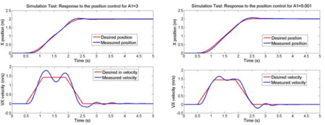
which we consider optimal to our application. In the Figure 11 we show the results obtained to this set of gains values. Note that the position error is small, for which, the overshoot does not pass 5%. As well, a good performance is noted for the speed, for which, we retrieve 10% of overshoot, with slightly oscillations, what does not bring prejudice to the system’s stability.
In our procedure, the next step, was to verify the behavior of the control when performing different smooth paths. The experimental results we show are obtained with Matlab simulation and on real flights carry out in our lab environment.
4 Experimental results
In this paper we present three cases: a sequence of waypoints designing a square, which objective is to show position error’s quality; a circle, which objective is to show the adaptability of the backstepping control, hence when the speed module reference remains constant; and a spiral reference path, showing the efficiency of the backstepping control law to drive movement on the three axes (x, y, z).
Path tracking simulation
We claim that this simulation test is pertinent to validation : one can verify the sequence on automatic paths generation and the quality of the control law developed in terms of position error.
The Figure 12 shows the trajectories performed by the quadrotor in simulation for the three paths cases. Note that, the position error is really small in the three cases. The Figure 13 shows the position error. Note that this error is small for the three axis, even for z. It can be explained by the fact that even for variations on x and y, the forces computed by the control law taken into account the thrust compensation over the z axis. The backstepping control law allows to anticipate falling down on z, what can happens when a movement on x and y is required, and correct this effect before it occurs.
Once the experimental results obtained in simulation was presented, one would present the testbed environment used to real flight tests. Note that the lab platform is a rich, complete and complex framework specially designed to easy test, in real flights experimentations, the quality of control laws developed.
(a) Position results for a squared path.
(b) Position results for a cir-cular path.
(c) Position results for a spiral path.
Fig. 13 Simulation results showing the sequence of target points.
Flight test results
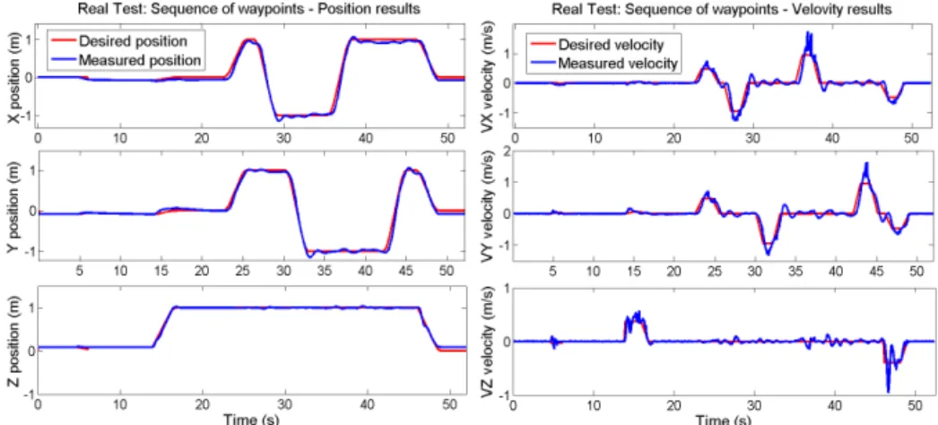
The Figure 14 shows the results obtained in real flight using the squared path as input reference. One can note the sequence of waypoints (w.r.t. the local frame) and the evolution of the measured position and speed. The regulation is well done, even on z axis. The control law assures a small overshoot (less than 5%), and a really week error on position, which is never corrected but we can consider this error acceptable. But, on the speed tracking, overshoot appears but are not dangerous for our application and for postion tracking purpose. The altitude tracking on the z position is well done, the effect of the non linear control is seen in this case. The thrust force that has to be applied is calculated depending the attitude of the quadrotor during all the flight (taking off, cruising, landing).
Fig. 14 Input references of position and speed, and measured ones when performing the squared path in real flight.
(a) 2D position result for a squared path. (b) 3D position results for a squared path. Fig. 15 Tracking smooth path flight results.
In the Figure 15 one can better visualize the trajectory performed in flight. Note that, there is a little gap on position in the x axis negative sens. This error could be explained by the fact that as the electronic used (for instance, wifi card, gumstix card, etc) are actually not placed in the center of the quadrotor structure, it displaces a little bit the center of mass. This error can be corrected modifying the Fdforce in consequence. Even with this little gap, we claim that the efficacy of the control law is proved with respect to our application. Moreover, as it is shown in Eq. 8, the yaw angle is not take into account on the backstepping control law computations, but by PID control used to the attitude control in flight experimentations. In this sense, the quality observed in real flight test is strongly attached to the regulation quality of the PID attitude control.
Note that, we do not claim or compare the backstepping control law against the embedeed (comercial) ARdrone speed control law. Our aim is to define a relevant control law, that will be base for further studies, specially focused in the definition of guidance algorithms. Guidance algorithms would provide position and/or speed references in constrained environments, which justifies the chosen of the backstep-ping control law. As it, this first study should concretize the definition of the control law that will be implemented in our futur robotic architecture.
5 Conclusion and future work
This paper presents a real flight application of the backstepping control law to path tracking aim. For it, the testbed environment and the hypothesis related with were presented. The identification of the quadrotor’s dynamic model was performed, us-ing this testbed, in order to well regulate the control’s gains (PID and backsteppus-ing) in Matlab. Hence, we do not claim any theoretical development. The principal ob-jective of this paper is to demonstrate the applicability of such control law in real flight testbed. In this sense, we have shown that such nonlinear control law works well even if a PID law for control attitude in used in a cascade way, with respect to our application case (indoor fligth).
In the future, the developed control law will be basis to a guidance component, in which, an convenient trajectory (result of a motion planning algorithm) will be used to guide the quadrotor in a constraint environment. Use this nonlinear control law present at least two advantages for the automated trajectory planning: the range of speed that can be used is larger in this case compared to the case where a linearized approach is used; and, a good position control is ensured, which is essential when moving in constrained environments.
References
1. Bouabdallah, S., Noth, A., Siegwart, R.: Pid vs lq control techniques applied to an indoor micro quadrotor. In: Intelligent Robots and Systems, 2004.(IROS 2004). Proceedings. 2004 IEEE/RSJ International Conference on, vol. 3, pp. 2451–2456. IEEE (2004)
2. Bouabdallah, S., Siegwart, R.: Backstepping and sliding-mode techniques applied to an indoor micro quadrotor. In: In Proceedings of IEEE Int. Conf. on Robotics and Automation, pp. 2247–2252 (2005)
3. Bouabdallah, S., Siegwart, R.: Full control of a quadrotor. In: Intelligent robots and systems, 2007. IROS 2007. IEEE/RSJ international conference on, pp. 153–158. IEEE (2007) 4. Das, A., Lewis, F., Subbarao, K.: Backstepping approach for controlling a quadrotor using
lagrange form dynamics. Journal of Intelligent and Robotic Systems 56(1-2), 127–151 (2009) 5. Das, A., Subbarao, K., Lewis, F.: Dynamic inversion with zero-dynamics stabilisation for
quadrotor control. IET control theory & applications 3(3), 303–314 (2009)
6. Doe, R.: The Orocos Project - Open RObot Control Software (2014). URL
http://www.orocos.org/
7. Hamel T Mahony R, L.R.O.J.: Dynamic modelling and configuration stabilization for an x4-flyer. In: IFAC 15th triennial World congress, Barcelona, Spain, (2002)
8. Kokotovie, P.V.: The joy of feedback: nonlinear and adaptive. IEEE Control Systems Maga-zine 12(3), 7–17 (1992)
9. Matthew, J., Knoebel, N., Osborne, S., Beard, R., Eldredge, A.: Adaptive backstepping control for miniature air vehicles. In: American Control Conference, 2006, pp. 6 pp.– (2006). DOI 10.1109/ACC.2006.1657678
10. Meier, L., Tanskanen, P., Heng, L., Lee, G., Fraundorfer, F., Pollefeys, M.: Pixhawk: A micro aerial vehicle design for autonomous flight using onboard computer vision. Autonomous Robots 33(1-2), 21–39 (2012)
11. Mellinger, D., Kumar, V.: Minimum snap trajectory generation and control for quadrotors. In: Robotics and Automation (ICRA), 2011 IEEE International Conference on, pp. 2520–2525 (2011). DOI 10.1109/ICRA.2011.5980409
12. Stevens, B.L., Lewis, F.L.: Aircraft control and simulation. John Wiley & Sons (2003) 13. Vago Santana, L., Brandao, A., Sarcinelli-Filho, M., Carelli, R.: A trajectory tracking and 3d
positioning controller for the ar.drone quadrotor. In: Unmanned Aircraft Systems (ICUAS), 2014 International Conference on, pp. 756–767 (2014). DOI 10.1109/ICUAS.2014.6842321