O
pen
A
rchive
T
OULOUSE
A
rchive
O
uverte (
OATAO
)
OATAO is an open access repository that collects the work of Toulouse researchers and
makes it freely available over the web where possible.
This is an author-deposited version published in :
http://oatao.univ-toulouse.fr/
Eprints ID : 15051
The contribution was presented at :
http://sites.ieee.org/africon2015/
To cite this version :
Demilew, Samuel Asferaw and Ejigu, Dejene and Da Costa,
Georges and Pierson, Jean-Marc Range-free selective anchor node center of the
smallest communication overlap polygon localization algorithm in wireless networks.
(2015) In: 12th edition of IEEE AFRICON 2015, 14 September 2015 - 17 September
2015 (Addis Ababa, Ethiopia).
Any correspondance concerning this service should be sent to the repository
administrator:
[email protected]
Range-free Selective Anchor Node Center of the
Smallest Communication Overlap Polygon
Localization Algorithm in Wireless Networks
Samuel Asferaw Demilew and
Dejene Ejigu
IT Doctoral Program,
Addis Ababa University Addis Ababa, Ethiopia
[email protected] & [email protected]
Georges Da-Costa
and Jean-Marc Pierson
Laboratoire IRIT UMR 5505,
Université Paul Sabatier Toulouse, France
[email protected] & [email protected]
Abstract— This paper presents a range-free selective anchor node center of the smallest communication overlap polygon localization algorithm in wireless networks. The algorithm is range-free which does not require ranging devices. To estimate the location of unknown (location unaware) nodes it uses node connectivity based on selected anchor (location aware) nodes. The algorithm first selects appropriate anchor nodes. Then, the True Intersection Points (TIPs) constituting the vertices of the smallest communication overlap polygon (SCOP) of these selected anchor nodes' communication ranges are found. Finally, the location of the unknown node is estimated at the center of the SCOP which is formed from these TIPs. The algorithm performance is evaluated using MatLab simulation and compares favorably to state-of-the-art algorithms: Centroid, improved version of CPE, Mid-perpendicular and CSCOP localization algorithms. The results show the proposed algorithm outperforms other state-of-the-art algorithms in location accuracy and it has reasonable computational complexity.
Keywords— anchor nodes; communication overlap polygon; range-free; localization algorithm; selective; true intersection points; false intersection points
I. INTRODUCTION
In world of wireless networks, locating where a given node physically positioned is a challenging one, yet essential for many applications. The usual technique is to install a Global Positioning System (GPS) receiver on each node. GPS is an energy hungry system whereas small wireless devices are usually energy-constrained [1] [2]. Hence, an alternative technique has to be proposed to alleviate the problem. As a result, range-free localization methods which are node connectivity-metric based techniques have proposed. These methods use the inherent radio-frequency (RF) communication capabilities of wireless nodes to geo-locate unknown nodes. The problem with such techniques is poor accuracy. Hence, research focus on increasing accuracy for these methods by proposing different range-free geo-localization algorithms.
In this paper, we propose selective anchor node range-free geo-localization algorithms: Selective two Anchor Nodes Center of the Smallest Communication Overlap Polygon and Selective three Anchor Nodes Center of the Smallest Communication Overlap Polygon. In the first algorithm we select two appropriate anchor nodes where as in the second one we select three among the set of neighbor anchor nodes to estimate the position of an unknown node. These anchor nodes transmit periodic beacon signals and unknown nodes use simple node connectivity metric to localize themselves. The core principle of our localization algorithm is first selecting appropriate anchor nodes then to find the SCOP that forms the communication range overlap of these selected anchor nodes. Finally, we take the center of this polygon as the estimated position of unknown node, Nx.
The performance of the proposed algorithms is compared with the well-known Centroid [3], improved, simplified and distributed version of CPE (Improved CPE) [7] [8], Mid-perpendicular [9] [10], and CSCOP [11]algorithms to compare the level of location accuracy and computational cost.
The rest of the paper is organized as follows: Section II reviews related works. Section III presents the localization technique of the proposed algorithms. Section IV provides a MatLab performance evaluation and computational complexity of the proposed algorithms. Finally, Section V offers a conclusion and future work.
II. RELATED WORKS
The popularity of wireless networks and the rapid increase of the Location Based Applications (LBAs) in recent years has greatly raised research attention on wireless node localization. Generally, wireless node localization methods can be classified into two categories: range-based and range-free method [5]. A range-based method uses additional dedicated ranging devices, like timers, signal strength receivers, directional antennas and/or antenna arrays to locate nodes. Usually, this method may give a fine-grained result putting strict requirements on signal measurements and time synchronization. However, its ranging equipment results in high power consumption of the wireless nodes’ scarce battery.
Alternatively, range-free localization methods do not require any additional battery hungry ranging devices for
distance/angle measurements among nodes. They use node connectivity and appropriate range-free localization algorithms. As a result, they do not consume high battery which makes them more appropriate to energy constrained wireless nodes localization. Nevertheless, their accuracy is poor. Due to this, research focuses on techniques to improve their accuracy. Range-free localization methods can be further categorized into two classes: local and hop-counting methods [1] [5].
In the first type, to estimate its own location the unknown node collects the location information of its neighbor anchor nodes. For example, in the Centroid algorithm [3], each wireless node estimates its location as the centroid of the locations of its neighbor anchor nodes. It can give good accuracy if anchor nodes are regularly positioned [9] [10]; however, if this is not the case, it gives low accuracy.
The APIT technique [6] was proposed by He et al. This technique divides the network environment into triangular regions between anchor nodes. Every sensor node determines its relative location based on the triangles and estimates its own position as the center of gravity of the intersection of all the triangles where the node may reside. However, APIT necessitates long-range anchor node stations and costly high-power transmitters.
The Convex Position Estimation (CPE) [4] algorithm, to advance the accuracy of the Centroid Algorithm, was first proposed by Doherty et al. The authors present an optimization model to locate the unknown node. The core principle of this algorithm is to find the smallest rectangle that bounds the overlapping communication range of anchor nodes. Then, it takes the center of this rectangle as the estimated location of the unknown node, Nx. The problem; however, is how to find
the smallest rectangle. The authors propose an abstract optimization model to get the smallest rectangle.
The original CPE algorithm is a centralized method because the resource-constrained unknown node is unable to do the large and complex calculations demanded by the optimization process. Consequently, all unknown nodes are necessitated to send the collected node connectivity information to a centralized controller. Then, the centralized controller calculates the location of each unknown node and transmits the estimated positions back to the corresponding unknown nodes resulting in high traffic and bottlenecks. In other words, the original CPE algorithm scales poorly when the network increases. Nevertheless, to overcome the problem of original CPE algorithm researchers [7] [8], have proposed an improved, simplified and distributed version of the original CPE algorithm. To find the smallest rectangle, unlike the original CPE algorithm, the improved version finds an Estimated Rectangle (ER) which bounds the SCOP. Then, the center point of ER is taken as the estimated location of the unknown node.
To advance the accuracy of Centroid and Improved CPE algorithms, other works [9] [10] have proposed Mid-perpendicular algorithm. The core principle of this algorithm is to get center of anchor nodes’ communication overlap by using mid-perpendicular lines on the three sides of a triangle made from the three anchor nodes. The cross point of the three
mid-perpendicular lines is taken as the estimated position of unknown node, Nx. As number of anchor nodes increase
beyond three, any three of them can give estimated position; therefore, as many as
C
n3 estimated locations of the unknown node can be generated, where n is number of anchor nodes. Consequently, the algorithm considers the average of all these positions as the final estimated position. Thus, this algorithm is computationally complex.Later, Demilew et al. [11] have proposed Center of the Smallest Communication Overlap Polygon (CSCOP) algorithm. The core principle of this localization algorithm is to find the SCOP forming the communication range overlap of anchor nodes. Then, it takes the center of this polygon as the estimated position of unknown node Nx. To achieve this, it
introduces the concept of TIPs to pinpoint the vertices of the SCOP. Centroid of vertices (or TIPs) of the SCOP is the location of the unknown node. Unlike both original CPE and its improved version which look for a rectangle that bounds the SCOP, CSCOP algorithm finds SCOP itself. This helps CSCOP algorithm to improve the localization accuracy relative to others.
A second type of range-free geo-localization method is hop-counting (also known as DV-Hop) method. It was first proposed by Niculescu and Nath [12]. In this method each unknown node in the network requests its neighboring anchor nodes to give their estimated hop sizes and then attempts to get the smallest hop count to its neighbor anchor nodes. Then, every unknown node estimates its distances to neighbor anchor nodes using the hop count. Finally, the unknown nodes use trilateration to estimate their location depending on the estimated distances to any three appropriate neighbor anchor nodes. There are many follow-up studies on DV-Hop method [13] but our focus is on the first type of method.
III. SELECTIVE ANCHOR NODECENTER OF THE SMALLEST
COMMUNICATION OVERLAP POLYGON LOCALIZATION
ALGORITHM
In this section, we introduce selective anchor node CSCOP algorithm. The core principle behind this selective anchor node CSCOP algorithm is selecting the anchor nodes which are the main contributors of neighbor anchor nodes smallest communication overlap polygon. As CSCOP algorithm works starting with 2 neighbor anchor nodes, we look selective 2 and selective 3 anchor nodes CSCOP algorithms, respectively.
A) Selective two Anchor Nodes CSCOP Localization Algorithm
Here, we select two appropriate neighbor anchor nodes which contribute better to the formation of SCOP. In Fig. 2, we have 3 neighbor anchor nodes of normal node Nx: A1, A2, and
A3. In this figure we see the SCOP (shaded area) of the 3
neighbor anchor nodes is actually formed from the communication overlap of the two neighbor anchor nodes: A1
and A3.
More distinctively, we can characterize these 2 neighbor anchor nodes as follows: they have the longest distance between them compared with any other two anchor node pairs in the entire neighbor anchor nodes distribution. In this figure,
A1 and A3 have the longest distance between. We can find
these two anchor nodes by using (1). Like other related range-free algorithms (Centriod, CPE, Mid-perpendicular, and CSCOP), Selective Anchor Node CSCOP also assumes neighbor anchor nodes have the same communication range and periodically beacon their location. To generalize, following the same steps, we can select 2 appropriate anchor nodes among k neighbor anchor nodes, when k is greater than two. Here is the program procedure for the Selective two Anchor Nodes CSCOP localization algorithm:
B) Selective three Anchor Nodes CSCOP Localization Algorithm
In Fig. 3, we have 4 neighbor anchor nodes to unknown node, Nx: A1, A2, A3 and A4. In this figure we see the SCOP
(shaded area) formed by the 4 neighbor anchor nodes is actually formed from the communication overlap of the three neighbor anchor nodes: A1, A2 and A3. In general, the three
farthest neighbor anchor nodes (A1, A2 and A3) are the main
contributors to the smallest communication overlap polygon. Characteristically, we can characterize these 3 neighbor anchor nodes as follows: 1) the first two are identified as we have discussed in Selective two Anchor Nodes CSCOP Algorithm step. 2) The third neighbor anchor node is one with longest perpendicular distance from the line connecting the two farthest anchor nodes. In the figure, the two farthest neighbor anchor nodes are A1 and A3. Other anchor nodes in the figure
are A2 and A4. Comparing their perpendicular distance to a line
connecting A1 and A3, clearly, A2 (with 10m distance) has a
longer distance than A4 (with 2m distance). So, the third
neighbor anchor node which contributes more to the formation of the smallest communication overlap polygon is A2.
Following the same procedure, we can select the three best neighbor anchor nodes which contribute most to the smallest communication overlap polygon among k number of neighbor anchor nodes when k is greater than 3.
Here is the program procedure of Selective three Anchor Nodes CSCOP Algorithm. In its program procedure, first, unknown node, Nx computes the distance between any two
neighbor anchor nodes using distance equation (1) below which is derived from the Pythagorean Theorem. To find the distance between two points
(
x
1, y
1)
and(
x
2, y
2)
, all that one needs to do is use the coordinates of these ordered pairs and apply the distance formula. If there are k neighbor anchor nodes, there will beC
n2distances in total. By comparing these distances, the unknown node, Nx can find out the two farthestneighbor anchor nodes; for example, represented as Ai and Aj.
(
)
(
)
2 1 2 2 1 2x
y
y
x
d
=
−
+
−
( )
1
Where, d is distance between two points;(
x
1, y
1)
and(
x
2, y
2)
are coordinate points of two different points.Then, Nx looks for the third neighbor anchor node which is
farthest to the line connecting Ai and Aj among all other
neighbor anchor nodes except Ai and Aj using (2). Assuming
the equation of the line connecting the two farthest points is
0
=
+
+
By
C
Ax
and a point is(
m,
n
)
, then, a perpendicular distance between the point and the line can be calculated using (2), where d is distance between the line and the point. 2 2B
A
C
Bn
Am
d
+
+
+
=
( )
2
Finally, the unknown node, Nx can compute its positionusing CSCOP algorithm based only on the three selected neighbor anchor nodes: Ai, Aj and Am. Fig. 4 below illustrates
the program procedure of Selective three Anchor Nodes CSCOP algorithm:
Fig 3. Principle of Selective three Anchor Nodes CSCOP Algorithm
Fig. 2 Principle of Selective two Anchor Nodes CSCOP algorithm
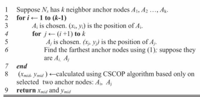
Algorithm: Selective two Anchor Nodes CSCOP
1 Suppose Nx has k neighbor anchor nodes A1, A2 …, Ak.
2 for i ĸ 1 to (k-1)
3 Ai is chosen. (xi, yi) is the position of Ai.
4 for j ĸ (i +1) to k
5 Aj is chosen. (xj, yj) is the position of Aj.
6 Find the farthest anchor nodes using (1); suppose they
are Ai, Aj
7 end
8 (xmid, ymid ) ĸcalculated using CSCOP algorithm based only on
selected two anchor nodes: Ai, Aj
9 return xmid and ymid
Fig. 1 Program procedure of Selective two Anchor Nodes CSCOP
IV. SIMULATION AND PERFORMANCE EVALUATION
In this section accuracy performance of both our Selective Anchor Node CSCOP localization algorithms are compared with the state of the art algorithms (Centroid, Improved CPE, Mid-perpendicular, and CSCOP). Parameters: average location error and probability distribution of location error are used to compare the algorithms. In the simulation MATLAB is used with ideal scenarios: ideal radio propagation without path loss or interference, no mobility for nodes, and no frame collisions. A special simulation area is configured to make sure the anchor nodes are located inside the range of the unknown node, Nx.
The radius is taken as the communication range of nodes. To make anchor nodes in the communication range of the unknown node, we set the side length of the square simulation area to be “2 × range” and we assume the unknown node locates at the center of the simulation area so it is in a radio range with any anchor node in the simulation area. Assuming the unknown node Nx has communicated with the anchor nodes
and knows their location.
Using respective algorithms: Centroid, Improved CPE, Mid-perpendicular, CSCOP, Selective two Anchor Nodes CSCOP, and Selective three Anchor Nodes CSCOP, unknown node Nx calculates its estimated location. The accuracy of these
algorithms is quantized by the metric “location error” and “location error % radio range” where the location error is the
distance between Nx’s estimated position and the real position.
The “location error % radio range” is obtained as the percentage of location error by the node radio range. Lower location error always indicates better accuracy. The unit is in meters.
To evaluate the accuracy of these localization algorithms, a comprehensive analysis on their average location error is essential. Moreover, probability distribution of location error which shows where most of the error occurs (either at average error value, maximum error value or minimum error value) has to be evaluated.
i) Average Location Error
Fig. 5 shows average location error performance of the algorithms. In the figure, Selective three Anchor Nodes CSCOP algorithm performs better than any other algorithms. It has big difference in performance compared to Selective two Anchor Nodes CSCOP algorithm. Both CSCOP and Selective three Anchor Nodes CSCOP perform better than the others. Comparing; however, the latter performs best. The figure also shows unlike other algorithms which look to at least 3 anchor nodes, both Selective two Anchors CSCOP and CSCOP algorithms work starting with two anchor nodes. As the number of anchor nodes increse (5, 6, 7, 8), the performance of both CSCOP and Selective three Anchor Nodes also increases when compared to others. Comparing the two, still the latter performce best.
ii) Probability Distribution of Location Error
Fig. 6 presents the probability distribution of location error of the algorithms. It is generated by using the MATLAB statistics toolbox normal fit function. In the figure, Selective three Anchor Nodes CSCOP has least location error distribution. When we compare state-of-the-art algorithms probability distribution of location error of our Selective three Anchor Nodes CSCOP has the highest probability (peak of its curve) with least location error value. The error value at this peak belongs to its average error which is occurring with highest probability while its maximum location error is occurring with a probability near to zero. Besides, it also has highest (equal to CSCOP) probability of minimum location error (which is zero error) making it more reliable than others. Contrary to this, our Selective two Anchor nodes CSCOP has
2 3 4 5 6 7 8 5 10 15 20 25 30 35
number of neighbor anchor nodes
lo c a ti o n e rr o r (% r a d io r a n g e ) Centroid improved CPE Mid-perpendicular CSCOP
Selective two Anchors CSCOP Selective three Anchors CSCOP
Fig. 5 Average location error (% radio range) Algorithm: Selective three Anchor Nodes CSCOP
1 Suppose Nx has k neighbor anchor nodes A1, A2 …, Ak.
2 for i ĸ 1 to (k-1)
3 Ai is chosen. (xi, yi) is the position of Ai.
4 for j ĸ (i +1) to k
5 Aj is chosen. (xj, yj) is the position of Aj.
6 Find the farthest anchor nodes using (1); suppose they
are Ai, Aj
7 end
8 end
9 for m ĸ 1 to k
10 Am is chosen. (xi, yi) is the position of Am
11 Find the anchor node with farthest perpendicular distance
to the line
j iA
A using (2); assume it is Am
12 end
13 (xmid, ymid ) ĸcalculated using CSCOP algorithm based only on
selected three anchor nodes: Ai, Aj and Am
14 return xmid and ymid
Fig. 4 Program procedure of Selective three Anchor Nodes CSCOP Algorithm
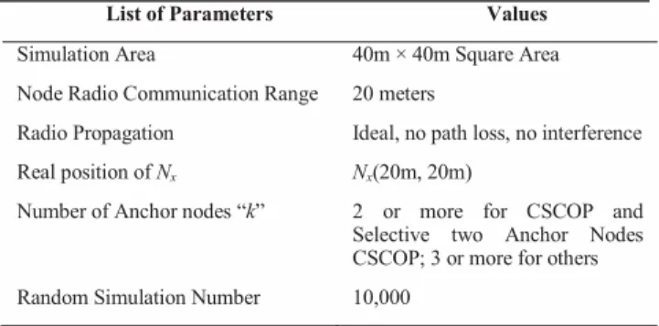
TABLE I. SIMULATION PARAMETERS
List of Parameters Values
Simulation Area 40m × 40m Square Area
Node Radio Communication Range 20 meters
Radio Propagation Ideal, no path loss, no interference
Real position of Nx Nx(20m, 20m)
Number of Anchor nodes “k” 2 or more for CSCOP and
Selective two Anchor Nodes CSCOP; 3 or more for others
poorer performance than the others, except, in minimum location error probability occurrence.
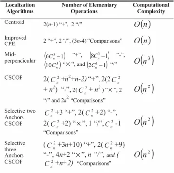
iii) Algorithms Computational Complexity
Table II shows the computational complexity of the algorithms. Assuming n number of anchor nodes, while Centroid has the lowest computational complexity, Mid-perpendicular has the highest. But, Centroid has lower accuracy than the latter. The question is how we can optimize both. Although computational complexity in ‘Big O’ notation is the same (as ‘Big O’ notation neglects the constants), our Selective three Anchor Nodes CSCOP has smaller number of elementary operations than CSCOP since it selects the best three anchors among n anchor nodes. This makes it better algorithm in optimizing both accuracy and complexity.
V. CONCLUSION
In conclusion, simulation results show Selective three Anchor Nodes CSCOP algorithm performs better than any other state-of-the-art algorithms in localization accuracy optimizing the trade-off between accuracy and computational cost.
As the SCOP is near to the unknown node it increases accuracy. It also defines the smallest search area where the target is situated. Its center is the estimated location of the unknown node. Currently, we are planning to investigate the algorithm farther in real radio propagation scenarios.
REFERENCES
[1] Lee et al. “Multihop range-free localization with approximate shortest path in anisotropic wireless sensor networks,” EURASIP Journal on Wireless Communications and Networking, 2014.
[2] Chi-Chang Chen, Chi-Yu Chang, and Yan-Nong Li, “Range-Free Localization Scheme in Wireless Sensor Networks Based on Bilateration,” International Journal of Distributed Sensor Networks, vol. 2013, Article ID 620248, 10 pages, doi:10.1155/2013/620248, 2013. [3] N. Bulusu, J. Heidemann, and D. Estrin. GPS-less Low-Cost Outdoor
Localization for Very Small Devices, IEEE Personal Communications, vol.7, no.5, pp. 28-34, 2000.
[4] L. Doherty, K.S.J. Pister, and L.E. Ghaoui. “Convex position estimation in wireless sensor networks”, in: Proceedings of IEEE INFOCOM ’01, Alaska, USA, Apr.2001, vol. 3, pp. 1655- 1663.
[5] F. Liu, X. Cheng, D. Hua, and D. Chen, “TPSS: a time based positioning scheme for sensor networks with short range beacons,” in Wireless Sensor Networks and Applications, pp. 175–193, Springer, New York, NY, USA, 2008.
[6] T. He, C. Huang, B. M. Blum, J. A. Stankovic, and T. Abdelzaher, “Range-free localization schemes for large scale sensor networks,” in Proceedings of the 9th Annual International Conference on Mobile Computing and Networking (MobiCom ’03), pp. 81–95, USA, September 2003.
[7] J.P. Sheu, J.M. Li, C.S. Hsu, “A Distributed Location Estimating Algorithm for Wireless Sensor Networks”, IEEE International Conference on Sensor Networks, Ubiquitous, and Trustworthy Computing (SUTC’06), vol.1, pp.1-8, June 2006.
[8] J.P. Sheu, P.C. Chen, and C.S. Hsu. A distributed localization scheme for wireless sensor networks with improved grid-scan and vector-based refinement, IEEE Transactions on Mobile Computing, 7(9) (2008), pp. 1110-1123.
[9] L. Gui, A. Wei, T. Val, “A two-level range-free localization algorithm for wireless sensor networks,” IEEE Conference on Wireless Communications Networking and Mobile Computing, pp. 1- 4, Chengdu, September 2010.
[10] L. Gui, T. Val, A. Wei, “A Novel Two-Class Localization Algorithm in
Wireless Sensor Networks,”,Network Protocols and Algorithms, vol. 3, no. 3 (2011).
[11] S. A. Demilew, G. Da-Costa, J. Pierson, D. Ejigu, “Novel Reliable Range-free Geo-localization Algorithm in Wireless Networks: Center of
the Smallest Communication Overlap Polygon (CSCOP),” 3rd
International IEEE Black Sea Conference on Communications and Networking, Constanta, Romania, 2015.
[12] D. Niculescu E B. Nath, “Ad hoc positioning system (APS),” in IEEE Global Telecommunications Conference (GLOBECOM’01), vol. 5, pp. 2926–2931, San Antonio, Tex, USA, November 2001.
[13] G. Song, D. Tam, “Two Novel DV-Hop Localization Algorithms for Randomly Deployed Wireless Sensor Networks,” International Journal of Distributed Sensor Networks, Hindawi Publishing Corporation, Article ID 107670, 2015. 0 5 10 15 20 25 30 35 40 45 0 0.01 0.02 0.03 0.04 0.05 0.06 0.07
location error (% radio range)
p ro b a b ili ty Centroid improved CPE Mid-perpendicular CSCOP
Selective two Anchors CSCOP Selective three Anchors CSCOP
Fig. 6. Probability distribution of location error (8 neighbor anchor nodes)
TABLE II. COMPUTATIONAL COMPLEXITY OF THE ALGORITHMS Localization Algorithms Number of Elementary Operations Computational Complexity Centroid 2(n-1) “+”, 2 “/”