O
pen
A
rchive
T
OULOUSE
A
rchive
O
uverte (
OATAO
)
OATAO is an open access repository that collects the work of Toulouse researchers and
makes it freely available over the web where possible.
This is an author-deposited version published in :
http://oatao.univ-toulouse.fr/
Eprints ID : 15052
The contribution was presented at :
http://sites.ieee.org/africon2015/
Official URL:
http://dx.doi.org/10.1109/AFRCON.2015.7331966
To cite this version :
Demilew, Samuel Asfraw and Ejigu, Dejene and Da Costa,
Georges and Pierson, Jean-Marc Novel range-free immune to radio range difference
(IRRD) geo-localization algorithm in wireless networks. (2015) In: 12th edition of
IEEE Africon 2015 (AFRICON 2015), 14 September 2015 - 17 September 2015
(Addis Ababa, Ethiopia).
Any correspondence concerning this service should be sent to the repository
administrator:
[email protected]
Novel Range-free Immune to Radio Range
Difference (IRRD) Geo-localization Algorithm in
Wireless Networks
Samuel Asferaw Demilew and
Dejene Ejigu
IT Doctoral Program Addis Ababa University
Addis Ababa, Ethiopia
[email protected] & [email protected]
Georges Da-Costa
and Jean-Marc Pierson
Laboratoire IRIT UMR 5505 Université Paul Sabatier
Toulouse, France
[email protected] & [email protected]
Abstract— This paper presents a novel range-free immune to radio range difference (IRRD) geo-localization algorithm in wireless networks. The algorithm does not require the traditional assumption of anchor (location aware) nodes that have the same communication range as it works with anchor nodes having homogeneous and/or heterogeneous communication ranges. It is rang-free - it utilizes node connectivity to estimate the position of unknown (location unaware) nodes using two or more anchor nodes. The algorithm works in two steps: in the first step, the True Intersection Points (TIPs) forming the vertices of the smallest communication overlap polygon (SCOP) of the anchor nodes are found. In the second step, it estimates the position of the unknown node at the center of the SCOP which is formed from these TIPs. The problem is first geometrically and mathematically modeled, then new localization approach that does not assume anchor nodes have the same radio range is proposed.
Keywords— anchor nodes; communication overlap polygon;
immune to radio range difference; localization algorithm; range-free; true intersection points
I. INTRODUCTION
Determining where a given wireless node physically positioned is challenging, yet vital for many applications. The common and easiest method is installing battery- hungry Global Positioning System (GPS) receivers on each wireless node but this contradicts with the fact that small wireless devices are usually energy-constrained [1] [2]. To overcome this problem, traditional range-free localization methods introduced usually assume anchor nodes have the same communication range, but in reality we have anchor nodes with different communication ranges. Thus, the problem of geo-localization of wireless nodes has to be addressed in a way which takes into consideration wireless nodes’heterogeneous communication (radio) ranges.
In this paper, we introduce a range-free localization method which is immune to anchor nodes’ communication range difference. It is based on nod connectivity by exploiting the inherent radio-frequency (RF) communication capabilities of wireless nodes. The neighbor anchor nodes (location aware nodes) transmit periodic beacon signals and unknown (location unaware) nodes use simple node connectivity metric to localize themselves. Unlike other algorithms, this algorithm i) works with two or more anchor nodes while others usually require at least three ii) works in both heterogeneous and homogeneous radio range of anchor nodes while others assume only the same iii) while estimating the position of the unknown node, it also defines the smallest search area where the unknown node resides, the smallest communication overlap polygon (SCOP).
The core principle of this geo-localization algorithm is to make the Center of the Smallest Communication Overlap Polygon (CSCOP) algorithm immune to radio range difference (IRRD) unlike other related algorithms which usually assume anchor nodes have the same radio ranges.
The rest of the paper is organized as follows: Section II reviews related works. Section III presents the geo-localization technique of the proposed algorithm in heterogeneous and/or homogeneous communication range of neighbor anchor nodes. Finally, Section IV offers a conclusion and a future work.
II. RELATEDWORK
The rapid increase of LBAs in wireless networks has stimulated research interest on the geo-localization of wireless nodes. Generally, methods of wireless node geo-localization can be categorized into two: range-based and range-free [5]. As its name indicates, range-based methods require additional dedicated ranging apparatus such as, signal strength receivers, timers and directional antenna and/or antenna arrays to locate unknown nodes. This technique may give good accuracy but on the cost of high battery consumption of scarce battery of wireless nodes.
On the contrary, range-free, as its name describes, demands no additional power hungry ranging apparatus for distance or/and angle measurements among nodes. Instead, it utilizes
already existing wireless node connectivity and appropriate range-free geo-localization algorithm. Nevertheless, this method usually results in coarse-grained location precision resulting in research targeting on techniques to enhance its precision. Range-free methods can be farther classified in to two classes: DV-Hop and local methods [5].
The Hop-counting (also known as DV-Hop) method was first proposed by Niculescu and Nath [11]. In this technique the unknown node requests its neighboring anchor nodes to provide their estimated hop sizes. Then, it attempts to find the smallest hop count to its neighbor anchor nodes. Then, every unknown node estimates its distances to neighbor anchor nodes using the hop count. Finally, trilateration is used by the unknown nodes to estimate their location based on the estimated distances to three selected neighbor anchor nodes. There are various follow-up studies on DV-Hop technique [12] but our interest is on the second type of technique.
A second type of range-free localization, local methods, is the focus of this work. In this method, an unknown node to estimate its location, it directly collects the location information of its neighbor anchor nodes. The first kind of range-free local method was first proposed by Bulusu et al. [3] called Centroid algorithm. In this algorithm, each wireless node estimates its position as the centroid of the positions of its neighboring anchor nodes. This algorithm gives good precision if the anchor nodes are regularly positioned; on the contrary, if the anchor nodes are not positioned regularly, it gives poor precision [9] [10].
To improve Centroid algorithm, later, He et al. proposed the APIT method [6]. This technique divides the network environment between anchor nodes into triangular regions. Then, every sensor node determines its relative location based on the triangles and estimates its own position as the center of gravity of the intersection of all the triangles where the node may reside. However, APIT requires long-range anchor node stations along with expensive high-power transmitters.
The Convex Position Estimation (CPE) algorithm was first proposed by Doherty et al [4] to enhance the accuracy of the Centroid algorithm. In this method, an optimization model was introduced to locate the unknown node. Finding the smallest rectangle that bounds the overlapping communication range of neighbor anchor nodes is the fundamental principle of this algorithm. Then, the centre of the rectangle is taken as the estimated location of the unknown node, Nx. To find the
smallest rectangle, the authors suggest an abstract optimization model. However, since the resource-constrained unknown node is unable to do large and complex calculations required by the abstract optimization process, the original CPE algorithm is a centralized method. Due to this, all unknown nodes are necessitated to transmit the collected node connectivity information to a centralized controller to compute their location first. Then, the centralized controller sends the estimated locations back to the corresponding unknown nodes. This results in high traffic and bottlenecks causing the original CPE algorithm to scale poorly.
However, an enhanced, simplified and distributed version of the original CPE (Improved CPE) algorithm was proposed [7] [8]. To find the smallest rectangle, unlike the original CPE,
the Improved CPE algorithm finds an Estimated Rectangle (ER) which bounds the SCOP. The estimated location of the unknown node is considered the centroid point of this ER.
To advance the accuracy of Centroid and Improved CPE algorithms, other researchers [9] [10] have proposed a Mid-perpendicular algorithm. The central principle of this algorithm is to find the centroid of anchor nodes’ communication overlap via mid-perpendicular lines formed from the three anchor nodes on their three sides of a triangle. Then, the estimated location is the cross-point of the three mid-perpendicular lines. When the number of neighbor anchor nodes increase beyond three, any three of them can be used to estimate position of the unknown node, Nx. Thus,
3
n
C
estimated positions of the unknown node can be generated, where n is number of neighbor anchor nodes. Then, the average of all these
C
n3 positions is regarded as the final estimated position. Due to this, the Mid-perpendicular algorithm is computationally complex.To improve the Mid-perpendicular algorithm, Demilew et al. [13] have proposed the Center of the Smallest Communication Overlap Polygon (CSCOP) localization algorithm. The fundamental principle of this algorithm is to get the SCOP formed from the communication range overlap of neighbor anchor nodes. Then, it takes the center of SCOP as the estimated location of unknown node. Unlike both the Original CPE and Improved CPE which look for a rectangle that bounds the SCOP, CSCOP algorithm finds SCOP itself. This helped CSCOP algorithm to advance localization accuracy, but like other related algorithms it also assumes neighbor anchor nodes have the same communication ranges.
However, this work tries to break this traditional assumption (that says anchor nodes have the same communication range) and looks for an algorithm which is immune to anchor nodes’ communication range difference (an algorithm which works with both homogeneous and/or heterogeneous communication ranges of anchor nodes).
III. IMMUNETORADIORANGEDIFFERENCE(IRRD) GEO-LOCALIZATIONALGORITHM
Range-free local methods: Centroid, Original CPE, Improved CPE, Mid-perpendicular and CSCOP localization algorithms all assume anchor nodes have the same communication ranges. To break this traditional assumption, we propose geo-localization algorithm which is immune to radio range difference (IRRD).
This algorithm works in the same steeps as CSCOP algorithm but in a different environment. While CSCOP assumes anchor nodes have the same communication range, this algorithm breaks this traditional assumption and makes CSCOP to work with anchor nodes having homogeneous and/or heterogeneous communication ranges.
Like CSCOP localization algorithm, it works in 2 steps: In first step, it finds the SCOP where the unknown node resides; in the second step, it estimates the position of the unknown node, Nx at the center of this pinpointed SCOP. Now, the
problem is how to make CSCOP immune to communication range difference of anchor nodes.
A) Finding the Smallest Communication Overlap Polygon (SCOP)
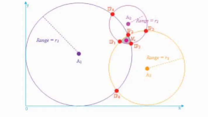
To illustrate how this algorithm works with anchor nodes that have communication range difference, let us look at Fig. 1 below:
In Fig. 1, the unknown node Nx has 3 neighbor anchor
nodes: (A1, A2, and A3) with their r1, r2, and r3 communication
ranges, respectively. Now, unknown node Nx’s neighbor
anchor nodes have different communication ranges (r1, r2, and
r3). Although unknown node’s neighbor anchor nodes have
different communication ranges, they are its neighbor anchor nodes. As a result, it locates inside the SCOP of these neighbor anchor nodes’ (the shaded area in the figure). Hence, we have to find SCOP first.
Finding SCOP works with two steps: 1) Finding Intersection Points (IPs)
The first step in pinpointing the SCOP is finding IPs. Fig. 1 shows 3 neighbor anchor nodes for the unknown node, Nx. In
other words, we have 3 circles (A1, A2, and A3) with radii r1,
r2, and r3, respectively. Hence, to get IPs of these circles, we
solve for IPs of each circle with every other circle using (1). IPs of any given 2 circles could be 1, 2, or infinity. If it is infinity, the two circles are identical which means they are one and the same circle. Thus, any 2 different circles intersect either at 1 point as in Fig. 3(a) or at 2 points as in Fig. 3(b).
Where (xi, yi) and (xj, yj) are the positions of the two
anchor nodes involved in the calculation of IPs; ri andrj are the
communication ranges (radii) of the two anchor nodes involved, respectively. For instance, in Fig. 1, if we take A1
and A2, they intersect at IP3 and IP4. In Fig. 1, we have six IPs:
IP1, IP2, IP3, IP4, IP5, and IP6. The next question is how we
identify True Intersection Points (TIPs) from False Intersection Points (FIPs) among these IPs.
2) Finding True Intersection Points (TIPs)
The second step in pinpointing the SCOP is identifying TIPs from FIPs. The TIPs are the vertices of SCOP. Those IPs which form vertices of SCOP are identified as TIPs whereas those which do not are FIPs using (2), where (xIPi, yIPi) and (xj,
yj) are the co-ordinates of the IPs and anchor nodes’ location,
respectively;
r
j2 is communication range (r1, r2, …, rj) ofanchor nodes (A1, A2,…, Aj).
To identify TIPs, we compare the distances between each IPs to ever anchor’s position whether it is less than or equal to rj (respective communication range of anchor nodes) or not. If
IP’s distance to each anchor is less than or equal to rj, that IP is
identified as a TIP. If not, it is regarded as a FIP. For example, as we can look at Fig. 2, among those six IPs in Fig. 1, IP1, IP2,
and IP3 are identified as TIPs whereas IP4, IP5, and IP6 are
considered as FIPs. Finally, we take only TIPs (TIP1, TIP2, and
TIP3) because they form the vertices of the SCOP.
Let us look at the likely range of TIPs in the following figures: Fig. 3(a) confirms anchor nodes can form a single TIP which is the SCOP at the same time. This indicates the estimated and the real position of the unknown node is one and the same (0% location error) which holds true in theory but difficult to achieve in reality. On the other hand, it can be just 2 as indicated in Fig. 3(b); just 3 as in Fig. 2, or k as in Fig. 3(c), where k is number of anchor nodes involved. Fig. 3(b) also indicates the algorithm can work with just 2 anchor nodes.
Fig.2 Identifying True Intersection Points (TIPs) from False Intersection Points (FIPs)
(
)
2(
)
2 2 j j IPi j IPi x y y r x − + − ≤(
)
(
)
(
)
(
)
°¯ ° ® = − + − = − + − 2 2 2 2 2 2 j j j i i i r y y x x r y y x xFig.1 Finding Intersection Points (IPs)
( )
1
Fig. 3 SCOP as one, two, k TIPs
a) b) c)
B) The Center of the Smallest Communication Overlap Polygon
Once we identified TIPs as its vertices of SCOP, then we estimate the position of the unknown node, Nx at the center of
these TIPs (or SCOP). Assuming finally we have m number of TIPs: P1, P2....Pm identified by using (2), then, unknown node
Nx locates itself at the center of these TIPs using (3), where
)
,
(
x
TIP1y
TIP1 ,(
x
TIP2,
y
TIP2)
…(
x
TIPm,
y
TIPm)
are co-ordinates of TIPs and m is the number of TIPs. The resultCSCOP
x
andy
CSCOP is the location of the unknown node, Nx.(
)
(
)
¯
®
+
+
+
=
+
+
+
=
m
y
y
y
y
m
x
x
x
x
TIPm TIP TIP CSCOP TIPm TIP TIP CSCOP...
...
2 1 2 1( )
3
Fig. 4 summarizes the program procedure of immune to radio range difference (IRRD) localization algorithm.
IV. CONCLUSIONANDFUTUREWORK In conclusion, unlike other related algorithms, Immune to Radio Range Difference (IRRD) algorithm as its name suggests works with both heterogeneous and homogeneous
communication ranges of anchor nodes. Furthermore, this algorithm, like CSCOP also defines the smallest frontier where the unknown node resides which is the SCOP, formed from TIPs as its vertices. Its application goes to all wireless networks ranging from cellular to sensor networks. As a future work we are planning to implement the algorithm in the real radio propagation scenario.
REFERENCES
[1] Lee et al.: Multihop range-free localization with approximate shortest path in anisotropic wireless sensor networks. EURASIP Journal on
Wireless Communications and Networking 2014 2014:80.
[2] Chi-Chang Chen, Chi-Yu Chang, and Yan-Nong Li, “Range-Free Localization Scheme in Wireless Sensor Networks Based on Bilateration,” International Journal of Distributed Sensor Networks, vol. 2013, Article ID 620248, 10 pages, 2013. doi:10.1155/2013/620248 [3] N. Bulusu, J. Heidemann, and D. Estrin. GPS-less Low-Cost Outdoor Localization for Very Small Devices, IEEE Personal Communications, vol.7, no.5, pp. 28-34, 2000.
[4] L. Doherty, K.S.J. Pister, and L.E. Ghaoui. “Convex position estimation in wireless sensor networks”, in: Proceedings of IEEE INFOCOM ’01, Alaska, USA, Apr.2001, vol. 3, pp. 1655- 1663.
[5] F. Liu, X. Cheng, D. Hua, and D. Chen, “TPSS: a time based positioning scheme for sensor networks with short range beacons,” in
Wireless Sensor Networks and Applications, pp. 175–193, Springer,
New York, NY, USA, 2008.
[6] T. He, C. Huang, B. M. Blum, J. A. Stankovic, and T. Abdelzaher, “Range-free localization schemes for large scale sensor networks,” in
Proceedings of the 9th Annual International Conference on Mobile Computing and Networking (MobiCom ’03), pp. 81–95, USA,
September 2003.
[7] J.P. Sheu, J.M. Li, C.S. Hsu, “A Distributed Location Estimating Algorithm for Wireless Sensor Networks”, IEEE International
Conference on Sensor Networks, Ubiquitous, and Trustworthy Computing (SUTC’06), vol.1, pp.1-8, June 2006.
[8] J.P. Sheu, P.C. Chen, and C.S. Hsu. A distributed localization scheme for wireless sensor networks with improved grid-scan and vector-based refinement, IEEE Transactions on Mobile Computing, 7(9) (2008), pp. 1110-1123.
[9] L. Gui, A. Wei, T. Val, “A two-level range-free localization algorithm for wireless sensor networks,” IEEE Conference on Wireless Communications Networking and Mobile Computing, pp. 1- 4, Chengdu, September 2010.
[10] L. Gui, T. Val, A. Wei, “A Novel Two-Class Localization Algorithm in
Wireless Sensor Networks”, Network Protocols and Algorithms, vol. 3, no. 3 (2011).
[11] D. Niculescu and B. Nath, “Ad hoc positioning system (APS),” in IEEE
Global Telecommunications Conference (GLOBECOM’01), vol. 5, pp.
2926–2931, San Antonio, Tex, USA, November 2001.
[12] D. Ma, M. J. Er, B. Wang, and H. B. Lim, “Range-free wireless sensor
networks localization based on hop-count quantization,”
Telecommunication Systems, vol. 50, no. 3, pp. 199–213, 2010. [13] S. A. Demilew, D. Ejigu, G. Da-Costa, J. Pierson “Novel Reliable
Range-free Geo-localization Algorithm in Wireless Networks: Center of the Smallest Communication Overlap Polygon (CSCOP),” 3rd
International IEEE Black Sea Conference on Communications and Networking, Constanta, Romania, 2015.
Algorithm: Immune to Radio Range Difference (IRRD) Algorithm
1 During a period t, unknown node Nx obtains the positions of k
neighbor anchors (A1, A2 …, Ak) and their communication range, rj.
2 (xi, yi) is a coordinate point, Intersection Point (IP), True
Intersection Point (TIP) 3 xcscop ĸ 0; ycscop ĸ 0
4 for i ĸ 1 to (k-1)
5 Ai is chosen. (xi, yi) is the position of Ai.
6 for j ĸ (i+1) to k
7 Aj is chosen. (xj, yj) is the position of Aj.
8 IP[(xi, yi)] ĸ calculated as (1) based on anchors Ai and Aj
9 C1 = C1+1 10 end for 11 end for 12 for i ĸ 1 to C1 13 IPi is chosen (xi, yi) is coordinate of IPi 14 for jĸ 1to k
15 k j is chosen (xi, yi) is the position of k j
16 TIP[(xi, yi)] ĸ calculated and checked as (2) based on IPs
computed and communication range r j
17 C2 = C2 + 1
18 end for 19 for i ĸ 1 to C2
20 do xcscop ĸ ( xcscop+TIP (xi)) ; ycscop ĸ ( ycscop + TIP(yi))
21 end for
22 xcscop ĸ xcscop /C2; ycscop ĸ ycscop / C2
23 return xcscop and ycscop
Fig. 5. Procedure of Immune to Radio Range Difference (IRRD) geo-localization algorithm