Sensitivity characterization of differential detectors for acquisition of weak GNSS signals

To link to this article

_{: DOI:10.1109/TAES.2015.130470}

URL :

http://dx.doi.org/10.1109/TAES.2015.130470

To cite this version

_{: Esteves, Paulo and Sahmoudi, Mohamed and Boucheret,}

Marie-Laure Sensitivity characterization of differential detectors for

acquisition of weak GNSS signals. (2016) IEEE Transactions on Aerospace

and Electronic Systems, vol. 52 (n° 1). pp. 20-37. ISSN 0018-9251

O

pen

A

rchive

T

OULOUSE

A

rchive

O

uverte (

OATAO

)

OATAO is an open access repository that collects the work of Toulouse researchers and

makes it freely available over the web where possible.

This is an author-deposited version published in :

http://oatao.univ-toulouse.fr/

Eprints ID : 17184

Any correspondence concerning this service should be sent to the repository

administrator:

staff-oatao@listes-diff.inp-toulouse.fr

Sensitivity Characterization of

Differential Detectors for

Acquisition of Weak GNSS

Signals

PAULO ESTEVES

MOHAMED SAHMOUDI, Member, IEEE

Institut Sup´erieur de l’Aeronautique et de l’Espace Toulouse, France

MARIE-LAURE BOUCHERET, Member, IEEE

´

Ecole Nationale Sup´erieure d’ ´Electronique, d’ ´Electrotechnique, d’Informatique, d’Hydraulique, et de T´el´ecommunications Toulouse, France

In this paper, we assess the potential of several forms of the postcoherent differential detectors for the detection of weak Global Navigation Satellite Systems (GNSS) signals. We analyze in detail two different detector forms, namely the pair-wise differential detector (PWD) and noncoherent differential detector (NCDD). First, we follow a novel approach to obtain analytic expressions to characterize statistically the PWD. Then, we use these results to propose a polynomial-like model fitted by simulation to the sensitivity loss experienced by the differential operation with respect to coherent summing. This sensitivity loss formula is also used to characterize the NCDD, which is shown to be more adequate than the PWD for the acquisition of GNSS signals. A comparison between the PWD, NCDD, and the traditional noncoherent detector (NCD) is also carried out in this study. The results highlight the superior performance of the NCDD over the NCD for the acquisition of weak signals. For the case of the PWD, its performance is sensitive to Doppler shift. The conclusions drawn from the simulation results are confirmed in the acquisition of real Global Positioning System L1 C/A signals.

This work was supported by the French Space Agency (CNES) and the Telecommunications for Space and Aeronautics laboratory (T´eSA), Toulouse, France.

Authors’ addresses: P. Esteves, M. Sahmoudi, Department of Electronics, Optronics, and Signal (DEOS), Institut Sup´erieur de l’Aeronautique et de l’Espace (ISAE), 31055 Toulouse, France; M.-L. Boucheret, ´Ecole Nationale Sup´erieure d’ ´Electronique, d’ ´Electrotechnique, d’Informatique, d’Hydraulique, et de T´el´ecommunications, 31000 Toulouse, France, E-mail: (paulo.esteves@isae.fr).

I. INTRODUCTION

The first step in the signal-processing chain of a Global Navigation Satellite Systems (GNSS) receiver is known as signal acquisition [1–3]. In this phase, the presence of a signal from a given satellite is decided based on the estimation of its unknown parameters, in particular its spreading code phase and Doppler offset. For the acquisition of signals with nominal power, integration over a duration equivalent to one period of the incoming signal’s spreading code is common usage for detection. For weaker signals, however, integration over several code periods is necessary [4, 5]. This is typically the case for positioning in urban canyons, where the signal can be degraded by different propagation phenomena including multipath [6], shadowing, signal blockage, and other sources of attenuation [7].

The maximum sensitivity gain is achievable by coherent integration of consecutive correlation outputs, obtained by correlating each code period of the signal with a code replica generated locally [8, 9]. Nevertheless, the coherent integration time is limited by factors such as residual Doppler offset, data bit transition, and the receiver’s processing capabilities [10, 11]. Therefore, after a certain number of coherent accumulations, transition to postcoherent integration strategies is usually employed to keep on increasing acquisition sensitivity. The most well-known, and generally applied, postcoherent integration strategy is noncoherent integration, in which the coherent outputs’ phase is discarded prior to further accumulation [1–3]. It is equally well-known, however, that noncoherent integration is less effective than coherent integration because the phase removal operation by squaring the in-phase and quadrature (I&Q) branches of the coherent output incurs a loss, known as squaring loss, that reduces the signal’s signal-to-noise ratio (SNR) [12, 13].

An alternative postcoherent integration approach is differential, or semicoherent, integration [14–22]. In this approach, the coherent outputs are not squared, but rather correlated with a previous output. The product of the two uncorrelated outputs is statistically less detrimental to SNR than the squaring operation, given the independence of the noise terms [14]. Different forms of detection schemes employing postcorrelation differential integration can be found in the literature [15–17]. One of the two main factors that distinguish these detectors is the generation of the differential outputs. Given the nature of the differential operation, each coherent output, except the first and last, may be used more than once. This results in a dependency between consecutive differential outputs that is remarkably difficult to characterize statistically. One approach to avoid this dependency is studied in [16], where each coherent integration output is used only once, in an approach termed as pair-wise integration. The drawback of this approach is that a reduced number of accumulations naturally lead to a smaller sensitivity increase than if all differential outputs were exploited [19].

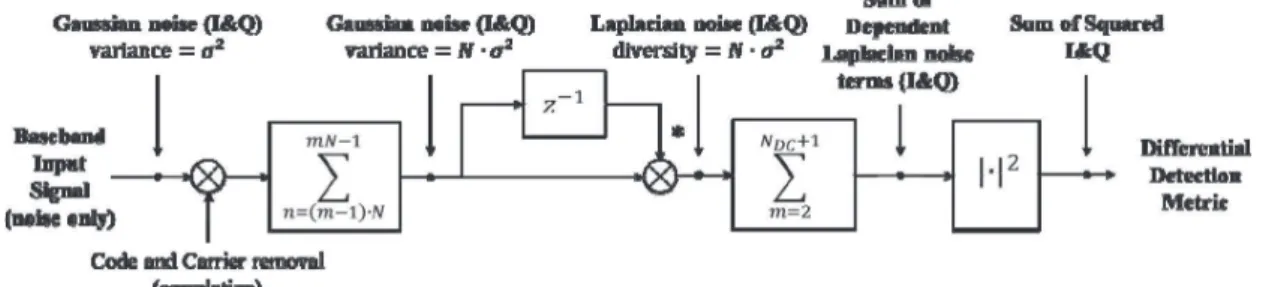
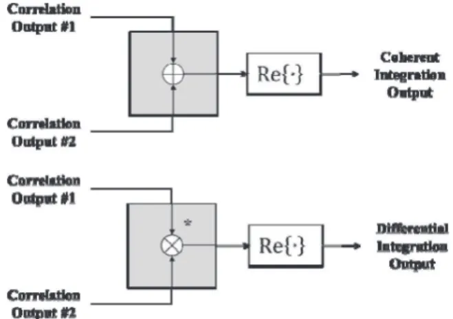
Fig. 1. Noncoherent differential detector block diagram and resulting noise distribution under no signal present case.

The second main factor that distinguishes differential detectors is the formulation of the detection metric from the differential integration outputs. In [15], only the in-phase branch of the differential integration output is considered in the detection test. A posterior evaluation of this detection metric in [17] notes that a residual Doppler offset leads to a partition of the useful signal power between the I&Q branches of the differential integration output, and a Doppler-robust noncoherent differential form is instead adopted in which the detection metric is obtained as the squared magnitude of the differential integration output (Fig. 1). Although this form

significantly improves the differential detection scheme performance in the presence of an unknown Doppler offset, its detection metric is obtained as the sum of two dependent random variables. This dependency once again complicates the statistical analysis of the detector output.

In [19], a complex mathematical approach is followed that enables the author to derive expressions for

characterizing the pair-wise detector (PWD) from [16] as well as the noncoherent differential detector (NCDD) from [17]. The author also notes, however, that, while exact, the expressions derived are of limited application due to the presence of functions that easily become both burdensome and inaccurate for a high number of differential accumulations. An equally complex analysis of differential detectors with similar results is also found in [18]. The approach that is frequently followed in the analysis of differential detectors is to resort to the central limit theorem (CLT) through which the noise terms resulting from differential integration can be approximated by a Gaussian distribution for a sufficiently high enough number of integrations [20, 21]. In [19], the author also develops a Gaussian approximation for each detector and points out the risk of employing this approximation for a low number of accumulations, given that the actual distributions of the I&Q components of the differential operation are heavier at the tails than the Gaussian distribution, leading to large inaccuracies in the threshold-setting process.

Both the multitude of existing differential detector forms and the complexity of their statistical

characterization have been obstacles to the comparison of the two postcoherent integration approaches, i.e.,

noncoherent and differential. Although in several publications it has been found that differential detectors are a preferable choice for weak signals acquisition, it was not until [22] that a formal comparison between the sensitivity losses of the squaring and differential operations was encountered. The approach developed in [22] is revised and consolidated in this paper.

In this study, we analyze the PWD and NCDD, and propose new approaches for the characterization of both. First, we analyze the PWD form by using a sum of weighted Laplace distributions to characterize this detector in the absence of signal, making use of the fact that the output of the differential integration results in a noise term following Laplace distribution. This analysis allows deriving an expression that can be used for setting the detection threshold, alternative to the one proposed in [16]. Under the alternative signal-present hypothesis, the Gaussian approximation is followed, not without first justifying its adequate use exclusively under this condition. We then make use of the results obtained to proceed to the assessment of the sensitivity of the NCDD detection scheme. Given the complexity of the statistical analysis of this detector (Fig. 1), we evaluate its detection performance by introducing and making use of a

sensitivity loss formula of this detector by evaluating the gain of each operation performed inside this detector. The final sensitivity loss formula is obtained through a polynomial fit of simulation results and validated by the theoretical results for the PWD. This formula finally allows performing a formal comparison between the two postcoherent integration strategies, also validated in the acquisition of real Global Positioning System (GPS) L1 C/A signals.

This paper is organized as follows. Section II introduces the signal model employed and describes the coherent processing of the input signal. In Section III, the PWD is characterized, showing the Laplacian nature of the differential operation output under noise-only conditions. In Section IV, the performance of the NCDD in the acquisition of weak GNSS signals is assessed. In Section V a comparison between the noncoherent detector (NCD) and the NCDD is carried out. Finally in Section VI, the conclusions are validated with real GPS L1 C/A data. Section VII concludes the paper.

Fig. 2. Coherent processing block of GNSS signal.

II. SIGNAL MODEL AND COHERENT SIGNAL PROCESSING

The goal of the acquisition module of a GNSS receiver is to detect the presence of a signal while providing a first coarse estimate of the incoming signal’s unknown code phase and Doppler shift. In stand-alone receivers, this estimation is usually accomplished using

maximum-likelihood estimation, testing several candidate code phases and frequency values within a given

uncertainty range. For this, the first two operations within acquisition are the despreading of the incoming signal and the conversion to baseband frequency using the candidate code phase/Doppler shift pair of values. The combination of the two operations and the posterior accumulation is known as correlation or coherent signal integration when more than one code period is used in this process. The coherent processing chain of a GNSS signal s[·] is shown in Fig. 2 and is represented as:

S¡ˆζi, ˆfdk¢ = N −1 X n=0 s [nTs]· c£¡n − ˆζi¢ Ts¤ · e−j 2π ˆfdknTs, (1) where ˆζiis the ith candidate code phase (code delay), ˆfdk

is the kth candidate demodulation frequency, c[·] is the spreading code, Tsis the sampling period, N is the number

of samples to be coherently accumulated (equal to the product of the number of samples per code period Nsand

the number of coherently integrated code periods Ncoh),

and S( ˆζi, ˆfdk) is the correlation output for the candidate

satellite, code phase, and demodulation frequency. The input signal is of the form:

s [nTs]= A · d [nTs− ζ Ts]· c [nTs− ζ Ts]

· ej2π fdnTs+φ0

+w [nT∼ s] , (2)

where A stands for the signal amplitude, ζ and fd,

respectively, denote the true code phase and frequency of this specific signal, d[·] = ±1 is the navigation data included in the signal, φ0represents the initial signal

phase offset, and_{w[·] is the noise component introduced}∼ by the communication channel that can be modeled as complex-valued zero-mean white Gaussian noise. The probability distribution is given by [20]:

p_{(ℜ{w}, ℑ{}∼ _{w}) =}∼ 1 2π σ2exp à −ℜ{ ∼ w}2 2σ2 − ℑ{w}∼ 2 2σ2 ! , (3)

where ℜ{w} and ℑ{∼ w} denote, respectively, the real and∼ imaginary parts of_{w[·]. The noise variance σ}∼ 2is given by:

σ2= E©ℜ©w∼ª2

ª = E©ℑ©w∼ª2

ª = N0B, (4)

where E{·} is the operator for the expectation value, N_{0 = k · T0}is the single-sided noise power spectral density, k being the Boltzman constant and T0the noise

temperature, and B ≃ 1/Tsthe front-end filter bandwidth.

It should be noted that (2) represents the signal from a single satellite. Given the orthogonality of the different signals’ spreading codes, all other signals satellites visible to the receiver can be considered as an extra noise component included in (2). This signal structure is based on the GPS L1 C/A signal and will be used in the analysis presented in this paper. The extension to other signal structures, such as Galileo E1, is straightforward. Examples of acquisition applied to this signal structure can be found, e.g., in [23, 24].

Depending on the presence or absence of signal, the

mth coherent integration output Sm( ˆζi, ˆfdk) will either be

obtained as noise-only or as a function of signal plus noise, and can be expressed using the following statistical test:

( Sm ¡_ˆζ i, ˆfdk¢ = wm, H0 Sm ¡ ˆζi, ˆfdk¢ = sm ¡ ˆζi, ˆfdk¢ + wm, H1 (5) where H0corresponds to the case when the signal under

search is not present and H1is the alternative hypothesis.

Given the distribution of the input signal noise, the coherent integration output noise term wmis equally a

complex-valued zero-mean Gaussian random variable with variance σ_w2 _{= Nσ}2and distributed according to (3). Assuming that all the signal parameters are constant over the observation time, the signal component of the coherent integration output sm( ˆζi, ˆfdk) is obtained as:

sm

¡_ˆζ

i, ˆfdk¢ = A · N · d · R (1ζi)

· sinc¡1fd,k· NTs¢ · ej φm, (6)

φm= 2πm1fd,kN Ts+ φ0, (7)

where 1ζi = ˆζi− ζ and 1fd,k= ˆfdk − fdare,

respectively, the code phase and frequency offsets between the candidate and true parameters of the signal, and R(1ζ ) represents the autocorrelation of the signal spreading code evaluated at the offset 1ζ . Without loss of generality we assume that the data bit is constant over the coherent integration time. This assumption is not restrictive given the existence of techniques that deal with this issue, including detection algorithms, subdivision of coherent integration in two parts and taking the most likely one not to contain data bit transition, or running several parallel coherent integrations at different tentative data bit boundaries [25]. Even if no such techniques are applied, the mean attenuation of the coherent integration output is only around 1 dB for a signal integration time inferior to the data bit duration for the GPS L1 C/A signal [10].

From (6), the limitations of coherent integration can be observed. For very long coherent integration times, not only the navigation data bit can no longer be considered constant, but also the product 1fd,k· NTshas to be

bounded to prevent high attenuations due to the sinc roll-off. In order to prevent high frequency-derived attenuations, the 1fd,koffset must be reduced in the same

proportion as Ncohis increased, leading to a demanding

requirement in terms of frequency resolution and, consequently, number of candidate points to be searched. In order to avoid both high attenuations in the final detection metric and high computational burden, transition from coherent to postcoherent processing is usually applied. The next sections will detail the postcoherent differential integration processing.

III. STATISTICAL CHARACTERIZATION OF DIFFERENTIAL INTEGRATION

Given that coherent integration is limited by several factors, transition to postcoherent integration is required in order to efficiently detect the presence of weak signals. While the statistical characterization of noncoherent integration is well established and used in the GNSS literature, a similar and practical evaluation is still needed for differential integration. As mentioned in the

Introduction, attempts in the literature to characterize detectors employing postcoherent differential integration have repeatedly resulted in either highly complex expressions or simplifications through Gaussian

approximations. This fact becomes even more significant considering the variety of such detectors that can be envisaged. Three different differential detection schemes are considered in the course of this work:

1) Coherent differential PWD [16]: SP W D ¡ ˆζi, ˆfdk¢ = ℜ (_⌊NC/2⌋ X m=1 S2m ¡ ˆζi, ˆfdk¢ · S ∗ 2m−1 ¡ ˆζi, ˆfdk ¢ ) , (8) 2) Coherent differential detector (CDD) [15]:

SCDD ¡ ˆζi, ˆfdk¢ = ℜ (NC X m=2 Sm ¡ ˆζi, ˆfdk¢ · S ∗ m−1 ¡ ˆζi, ˆfdk ¢ ) , (9) 3) NCDD [17]: SN CDD ¡ ˆζi, ˆfdk¢ = ¯ ¯ ¯ ¯ ¯ NC X m=2 Sm ¡ ˆζi, ˆfdk¢ · S ∗ m−1 ¡ ˆζi, ˆfdk ¢ ¯ ¯ ¯ ¯ ¯ 2 , (10) where NCrepresents the number of available coherent

outputs. The differences between these three detectors are based firstly on the accumulation of the differential outputs (note the 2m index for each coherent integration output for the PWD) and secondly on the generation of the final detection metric, coherent or noncoherent, depending if the phase is removed prior to detection or not. The PWD form is the simplest to analyze due to the absence of

dependency terms both in the differential outputs accumulation as well as in the generation of the detection metric. On the contrary, the most difficult one to

characterize statistically is the NCDD. In this section, we analyze statistically the PWD that will afterward allow advancing to the characterization of CDD and NCDD.

In both original publications, [19, 26], the PWD detection metric has been expressed as the difference of two χ2random variables (central under H0and noncentral

under H1) to attempt its characterization. In this work, we

follow a different approach for the characterization of this detector, making use of the Laplace nature of the

differential operation output under H0and employing the

Gaussian approximation under H1. We will first

demonstrate that these are appropriate characterizations for this detection metric.

A. PWD Probability Density Function Under H0

Modeling the output of a detector under no signal present, only noise, allows establishing a threshold for deciding if a candidate signal is present or not with a certain degree of confidence, established by the acceptable probability of false alarm Pf a. In this case, the coherent

integration outputs consist solely of the accumulation of Gaussian noise terms, and the output of the PWD is:

SH_{P W D}0 ¡ˆζi, ˆfdk¢ = ℜ    NP W DC X m=1 S2m ¡_ˆζ i, ˆfdk¢ · S ∗ 2m−1 ¡_ˆζ i, ˆfdk ¢    = NP W DC X m=1 ℜ©w2m· w_2m−1∗ ª = NP W DC X m=1 ℜ©YH0,m ª = NP W DC X m=1 Y_H0,mI , (11) where NP W

DC = ⌊NC/2⌋ is the number of differential

integrations that can be performed for this detector having NCcoherent outputs available. As demonstrated in

Appendix A, the Y_HI_0,mterm is a zero-mean Laplace-distributed random variable with diversity parameter l equal to σ2

w. Its probability density function

(PDF) is given by [27]: fYI H0,m(y) = 1 2l· e −|y|λ ₌ 1 2σ2 w · e− |y| σ 2w, (12)

and the corresponding cumulative density function (CDF):

FYI

H0,m(y) =

1 2 h

1 + sgn (y)³1 − e−|y|l´i_{. (13)}

This way, the PWD detection metric under H0is

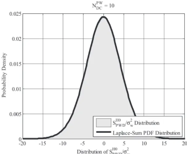
obtained as the sum of N_DCP W such Y_HI_0,mterms. Given the independency between the consecutive differential outputs characteristic of the PWD, the PDF of S_{P W D}H0 is that of the sum of independent Laplacian random variables. This

Fig. 3. Distribution of SH0_{P W D}for N_DCP W= 10 and PDF of sum of 10 independent Laplace random variables with λ = σ2

w.

PDF is known from [28] as:

f_SH0 P W D(y) = NP W DC−1 X k=0 Ã N_DCP W_{+ k − 1} k ! × e−|y|λ · ³ |y| λ ´NDCP W−k−1 2NP W DC+k·¡NP W DC − k − 1¢! · l , (14) and the respective CDF is found by integrating (14) with respect to y: F_SH0 P W D(y) = 1 2+ sgn (y) NP W DC−1 X k=0 Ã N_DCP W_{+ k − 1} k ! × γNP W DC−k ³ |y| l ´ 2NP W DC+k , (15)

where γa(·) is the lower incomplete Gamma function of

order a. The accuracy of this formulation can be asserted by comparing the histogram of simulation results with the theoretical distribution given by (14). This comparison is shown in Fig. 3 for N_DCP W _{= 10. As can be seen in this} figure, the PDF corresponding to the sum of Laplace random variables accurately matches the simulation results. It is now possible to set the detection threshold Vt h

for the PWD according to the specified Pf aby using (15)

and solving:

Pf a= 1 − FSP W D,H0(Vt h) . (16)

This characterization of the PWD under H0can be used as

an alternative to the existing formulas in [16, 19]. B. PWD PDF Under H1

Under H1, the signal under test is considered to be

present, and the detection performance of the detector as a function of the input signal power, as well as the threshold set via the H0analysis, is assessed. In the presence of

signal, the PWD detection metric results in: SP W DH1 ¡ ˆζi, ˆfdk ¢ = ℜ    NP W DC X m=1 S2m ¡ ˆζi, ˆfdk¢ · S_2m−1∗ ¡ ˆζi, ˆfdk ¢    = NP W DC X m=1 ℜ©s2ms∗_2m−1+ s2mw_2m−1∗ + w2ms_2m−1∗ + w2mw∗_2m−1 ª = NP W DC X m=1 ℜ©µm+ wY,m+ YH0,m ª = NP W DC X m=1 ℜ©YH1,mª . (17)

The first term, i.e., µm, is the deterministic component

originating from the product of the two signal

components, and the third term, i.e., YH0,m, was analyzed

in the previous section. The remaining term, i.e., wY,m, is

obtained as the sum of the products of the deterministic signal with Gaussian noise and is therefore a Gaussian random variable. Thus, the statistical analysis of the differential integration output under H1involves analyzing

the sum of a Laplace and a Gaussian random variable, dependent between them. If these two terms were

independent, their distribution could be directly expressed as a normal-Laplace random variable [29]; however, this is not the case. In [16] as in [19], it is suggested to rewrite ℜ{YH1,m} as the subtraction of two χ2random variables,

but this approach does not lead to a closed-form expression, having to resort to numerical methods to compute the integral term and obtain the final result. Instead, in [20], it is proposed to approximate ℜ{YH0,m}

by a Gaussian random variable under the claim of the CLT through which the summation of several such terms will tend to a normal distribution with variance equal to that of the individual terms. While this is not a recommended approach to follow under H0given the low precision at the

tails of the Gaussian approximation vis-`a-vis the requirement for the accurate threshold determination, it can be considered an acceptable approach under H1.

Furthermore, in [21] four different PDFs are fitted to the actual distribution of the differential integration outputs under H1, concluding that the Gaussian distribution is the

one that most accurately matches the true detector output distribution in these conditions. This will be especially true when the input signal power is high and the Gaussian noise term becomes much more significant than the Laplacian one.

From [27], the variance of a Laplace-distributed random variable is 2l2, which leads to:

var©ℜ ©YH0,mªª = 2σw4. (18)

Assuming stationarity of all parameters during the signal integration time, the variance of ℜ{wY,m} can be easily

seen to be given by:

var©ℜ ©wY,mªª = 2 · var {ℜ {smwm}} = 2 · |sm|2· σw2.

(19) This way, SH_{P W D}1 can be modelled as a noncentral Gaussian random variable with mean µSH1

P W D and variance σ 2 SH1 P W D given by: µ_SH1 P W D ≃ N P W DC · ℜ {µm} = NDCP W · |sm|2· cos¡2π1fd,kN Ts¢ , (20) σ_S2H1 P W D ≃ N P W DC ·¡ℜ ©wY,mª + ℜ ©YH0,mª¢ = NDCP W · 2σ 2 w·¡|sm|2+ σw2¢ , (21)

where once again the approximate equalities are obtained assuming stationarity of all parameters during the signal integration time. Evidently, this is not the case when dealing with real signals, but it is an essential assumption for the characterization of the detectors’ performance.

The drawbacks of the PWD detection metric are now remarked in (20) because not only is N_DCP W approximately only half of the number of differential integration outputs that can be generated, but also given 1fd,k 6= 0, a portion

of the signal power is allocated to the imaginary part of YH1,mand is therefore not useful. The expression for the

probability of detection Pdfor the PWD is finally obtained

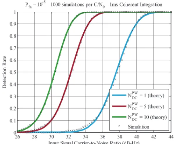
as: Pd,P W D = 1 q 2π σ2 SH1 P W D · ∞ Z Vt h exp      − ³ t − µSH1 P W D ´2 2σ2 SH1 P W D      dt =1 2erfc   Vt h− µSH1 P W D q 2σ2 SH1 P W D  , (22) where erfc(·) is the complementary error function, representing the tail probability of the standard normal distribution. To assess the accuracy of the fit provided by this expression, a comparison between the predicted and simulated detection rate for a GPS L1 C/A signal sampled at twice the chip rate is shown in Fig. 4 for N_DCP W _{= 1, 5,} and 10, employing 1-ms coherent integration (N = 2046) and 1fd,k= 1ζ = 0. The theoretical analysis is carried

by first calculating the threshold using (16) and then employing (22) to predict the detection probability, while the simulation analysis calculates the threshold based on the simulated noise distribution and then measures the detection rate as the percentage of threshold crossings for each carrier-to-noise (C/N0) value.

As shown in Fig. 4, the predicted PWD performance according to (22) is very close to the one observed in the simulations, which validates the Gaussian approximation under H1. The accuracy of this approximation can also be

observed by comparing the normal PDF and the histogram of the detector outputs. Two examples are shown in Fig. 5 From the plots in this figure, it is clear that the Gaussian approximation is very accurate for high input C/N0values

even for a low number of accumulations. This is due to the

Fig. 4. Comparison between theoretical and simulated detection probability for NP W

DC = 1, 5, and 10 (1 ms coherent integration,

1fd,k= 1ζ = 0).

higher influence of the cross-noise-signal multiplication, i.e., wY,min (17), with respect to the noise-only Laplacian

term. Contrarily, for weak signals and a low number of accumulations, the Gaussian fit is not an accurate representation of the detector output distribution, but the closeness between the two distributions is still high. In fact, the area matched in the top plot of Fig. 5 is close to 90%. This also explains why the difference between the predicted and simulated results in Fig. 4 is not substantial even for low C/N0values. Additional simulations confirm

that the Gaussian approximation becomes gradually more accurate for a higher number of accumulations, where the area match in these cases is even greater than for the two presented here. Alternatively, one may estimate the PDF of the detector under H1from data using nonparametric

kernel estimation with a cost of additional computation [30].

The expressions for the probability of false alarm and probability of detection derived in this section completely characterize the PWD. The derivation of similar

expressions for the CDD and NCDD is significantly more complex due to the rise of dependency between terms. Therefore, we follow a different approach in the next section to assess the performance of these two detectors by evaluating their sensitivity gain.

IV. SENSITIVITY OF DIFFERENTIAL DETECTORS In the previous section, the PWD has been studied, highlighting its drawbacks for GNSS signal acquisition, particularly in the presence of a nonzero residual Doppler offset in the coherent output. A more suitable detector in presence of Doppler frequency shift is the NCDD whose detection metric removes the phase information by a squaring operation as [17]: SN CDD ¡ ˆζi, ˆfdk¢ = ¯ ¯ ¯ ¯ ¯ NDC+1 X m=2 Sm ¡ ˆζi, ˆfdk¢ · S ∗ m−1 ¡ ˆζi, ˆfdk ¢ ¯ ¯ ¯ ¯ ¯ 2 , (23)

Fig. 5. Accuracy of Gaussian approximation of differential integration output under H1for NDCP W= 1 and C/N0= 34 dB-Hz (top) or

C/N0= 44 dB-Hz (bottom).

where NDC= NC− 1 is the number of differential

integrations achievable with this detector form having NC

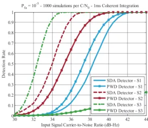
correlation outputs available. The advantage of this detector with respect to the PWD can be directly observed in simulations. In Fig. 6, the detection performance of the two detectors is compared for three different simulation scenarios whose details are shown in Table I. For scenario S1, where the residual Doppler offset is null and the same number of accumulations is performed for both detectors, the PWD outperforms the NCDD, due to the of the squaring loss paid by the NCDD. However, this gain with respect to the NCDD will be limited as the Doppler offset grows, according to (20). For scenario S3 in particular, where cos(2π 1fd,kN Ts) = 0, the nonzero detection rate

for the PWD at high input signal power is achieved merely due to the influence of the cross-signal-noise Gaussian terms wY,min (17).

Because the statistical characterization of the NCDD is not easy to accomplish, studies in literature commonly use the Gaussian approximation under both H0and H1

hypotheses. However, as previously noted, this cannot be considered a reasonable option under H0for a low number

of differential accumulations given the required precision

Fig. 6. Comparison of PWD and NCDD for simulation scenarios described in Table I.

TABLE I

Simulation Scenarios for Detectors Comparison in Fig. 6 Simulation Scenario

Simulation Parameters S1 S2 S3

Signal GPS L1 C/A

Sampling frequency 2.046 MHz

Coherent integration time 1 code period—1 ms/2046 samples

Number of code periods 2 6 11

Differential integrations NCDD 1 NCDD 5 NCDD 10

PWD 1 PWD 3 PWD 5

Residual Doppler offset 0 Hz 125 Hz 250 Hz

at the tails of the distribution. Instead we propose to follow an alternative to the formal statistical analysis of this detector, establishing a comparison with a reference scheme whose analysis is mathematically viable. This approach is followed in [31] for the characterization of the NCD applied to radar systems. In [31], a sensitivity loss term is defined that allows predicting the detection performance of a noncoherent detection scheme operating at a target receiver working point (Pd, Pf a) with respect to

the one that would be obtained if a coherent solution was instead applied. The formula provided in [31] is usually adopted in GNSS literature for analysis of the squaring loss of noncoherent integration [1, 4, 7]. The same procedure is followed in this section to propose a loss formula for the NCDD, i.e., LN CDD. This procedure was

previously followed in [22] and [32], but given the lack of accurate expressions for the statistical characterization of the differential operation, the formulas proposed were solely based on simulation data. Returning to the analysis described in the previous section, an analytical approach can now be followed to validate and complement the work in [22].

This section starts by reviewing the optimal GNSS detector as well as the procedure to derive a sensitivity loss formula with respect to this detector. Next, a formula for the differential integration loss is proposed, and the

sensitivity loss of the NCDD is obtained as a combination of the differential and squaring losses.

A. Sensitivity Loss of a Nonoptimal GNSS Detector 1) Methodology of Evaluation: The optimal detector in the presence of a stationary signal and known signal phase is the purely coherent detector (CD) [8]. The detection metric for the CD is defined as:

SCD¡ˆζi, ˆfdk¢ = ℜ (NC X m=1 Sm¡ˆζi, ˆfdk ¢ ) . (24) It should be noted that this detector is only possible to apply in theory given the assumption of knowledge of the input signal phase. However, it serves as a reference for the evaluation of the detection loss of nonoptimal, but practical, detectors. The equation that characterizes this detector’s performance is [31]: Pd,CD = 1 2erfc h erfc−1¡2Pf a¢ − p NCNssnrin i

=1₂erfc£erfc−1¡2Pf a¢ −√snrcoh¤ , (25)

where snrinand snrcohare, respectively, the SNR,

expressed in linear dimensions, at the detector input and after coherent integration (in this case coincident with the detector output), and Nsthe number of samples per code

period. Inverting (25), the SNR at the coherent integration output can be expressed as a function of the target working point:

snrcoh=£erfc−1¡2Pf a¢ − erfc−1(2Pd)

¤2 = Dc¡Pd, Pf a¢ . (26)

This SNR is also known as ideal detectability factor Dcand represents the minimum SNR at the coherent

integration output that allows detection of signal at the target receiver working point (Pd, Pf a). The minimum

input precorrelation SNR is then expressed as a function of Dcas:

snrin,min=

Dc

NcNs

. (27)

The product NcNsin this equation corresponds to the

gain of coherently integrating the NcNs signal samples

and is the maximum achievable signal integration gain. Consequently, the required input SNR, i.e., snrin,req, for

achieving a similar working point with detectors employing other integration approaches (such as noncoherent or differential integration), must always be higher than snrin,mingiven the nonideality of the

operations involved. A sensitivity loss characteristic of the nonideal detector Ldet ect orwith respect to the ideal

coherent one may then be expressed as [31]: Ldet ect or = snrin,req snrin,min = snrin,req· Ns Dc/Nc . (28) Given the linearity of the correlation operation, Ldet ect orcan also be interpreted as the ratio of the two

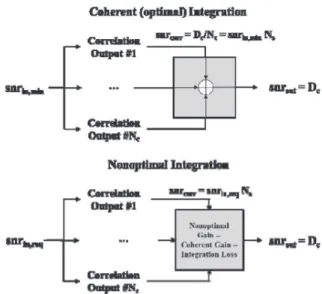
Fig. 7. Coherent (optimal) and nonoptimal integration strategies diagram and SNR measuring points.

correlation output SNRs (Fig. 7). This can also be noted in (28) because the product snrin,req· Nscorresponds to the

SNR at the correlation output of the nonoptimal detector and Dc/Nccorresponds to the SNR at the correlation

output of the CD. Finally, the required SNR to acquire a signal at a given working point with the nonoptimal detector can be expressed as:

SN Rin,req,dB = SNRin,min,dB+ Ldet ect or,dB

= 10 · log10

µ _D

c

NsNc

¶

+ Ldet ect or,dB. (29)

The ratio Dc/Nscorresponds to the input SNR that

would be required by the CD if only one code period would be available and can be denoted as snrin,min,Nc=1.

Equation (29) can then be rewritten as: SN Rin,req,dB= SNRin,min,Nc=1,dB

−¡10 · log10(Nc) − Ldet ect or,dB

¢ = SNRin,min,Nc=1,dB− Gdet ect or,dB(Nc) ,

(30) where Gdet ect orcorresponds to the detector sensitivity gain

of integrating a number Ncof code periods and is defined

as the difference between the ideal gain of coherent integration and the loss of the nonoptimal operations performed with respect to the ideal detector.

2) Application to the Squaring Loss: These expressions can be used in the quantification of the squaring loss Lsq

that is incurred by the phase-removal operation,

representing the price to pay in terms of additional input SNR for not knowing the input signal phase. In this case, the optimal detector is the square-law detector (SLD), whose detection metric is expressed as [8]:

SSLD¡ˆζi, ˆfdk¢ = ¯ ¯ ¯ NC X m=1 Sm¡ˆζi, ˆfdk ¢ ¯ ¯ ¯ 2 . (31)

The equation that characterizes the detection performance of the SLD is [19]: Pd,SLD= Q1 µ p 2NCNssnrin, q −2 ln¡Pf a¢ ¶ = Q1 µ p 2 snrcoh, q −2 ln¡Pf a ¢ ¶ , (32) where QK(a, b) is the Kth-order Marcum Q-function. The

squaring loss can now be expressed as the ratio between the input SNRs required by the two detectors in order to achieve similar detection performance:

Lsq= snrin,SLD snrin,CD = snrcoh,SLD snrcoh,CD = snrcoh,SLD Dc . (33) This loss can be promptly obtained by solving (26) and (32) for any (Pd, Pf a) pair and using the results in (33).

Nevertheless, solving these equations is a nontrivial mathematical process, and in [31], a simple approximation for Lsqis suggested: Lsq = snrcoh,SLD Dc ≃ 1 + 2.3 snrcoh,SLD ≃1 + √ 1 + 9.2/Dc 2 . (34)

The sensitivity gain of the SLD in the presence of Nc

code periods is then given by:

GSLD,dB(Nc) = Gcoh,dB(Nc) − Lsq,dB, (35)

where Gcoh(Nc) = Nc. As an example, the input signal

power required by the SLD for the acquisition of a single GPS C/A code period, sampled at twice the chip rate (Ns = 2046) and for a working point

(Pd, Pf a) = (0.9, 10−5), can be found through:

Dc,dB¡0.9, 10−5 ¢ =£erfc−1¡2 · 10−5¢ − erfc−1(2 · 0.9)¤2= 11.9 dB, Lsq,dB= 10 · log10 µ 1 +√1 + 9.2/Dc 2 ¶ = 0.6 dB, GSLD,dB(1) = Gcoh,dB(1) − Lsq,dB = −0.6 dB, SN Rin,SLD,dB= 10 · log10 µ Dc Ns ¶ − GSLD,dB(1) ≃ −20.6 dB.

Naturally, a very similar result is obtained by solving (32): 0.9 = Q1 µ p 2 · 1 · 2046 · snrin, q −2 ln¡10−5¢ ¶ ⇔ SNRin,dB ≃ −20.6 dB.

This approach can be generalized to any number of squaring operations and is the basis for obtaining the loss of the noncoherent integration scheme in [31]. This method of evaluating the nonoptimal detectors’ sensitivity loss differs from the traditional approach of calculating a

Fig. 8. Comparison for determination of differential operation sensitivity loss.

deflection coefficient as a measure of the output SNR. This approach has been followed for both the differential and noncoherent detection schemes in several studies such as [13, 21], but its inapplicability in these cases is explicitly illustrated in [33] and, therefore, is not considered here. B. Sensitivity Loss of the Differential Operation

In order to be able to quantify exclusively the loss of the differential operation with respect to coherent summing, the detection scheme employed in this analysis must avoid any other operations, in particular the squaring of the signal for phase removal. This can be achieved by concentrating all the signal power on the in-phase branch of the differential integration output (zero residual Doppler offset) and then taking just its real part as the detection metric (Fig. 8). By comparing the required input SNRs for the two schemes in Fig. 8, it is guaranteed that the difference in performance between both is exclusively due to the nonoptimality of differential operation with respect to coherent summing. The differential detector employed in this case corresponds to the CDD:

SCDD ¡_ˆζ i, ˆfdk¢ = ℜ (NDC+1 X m=2 Sm ¡_ˆζ i, ˆfdk¢ · S ∗ m−1 ¡_ˆζ i, ˆfdk ¢ ) . (36) As for the moment, we are focusing in the assessment of the sensitivity loss of a single differential operation, and the detection metric of interest is:

SCDD¡ˆζi, ˆfdk¢ = ℜ ©S2 ¡_ˆζ i, ˆfdk¢ · S ∗ 1 ¡_ˆζ i, ˆfdk¢ª . (37)

To characterize the sensitivity of this detector using its probability of detection, we need the PDF of the detection metric in (37) under H1. Because this detection metric is

equivalent to the PWD one for NP W

DC = 1, the results from

the previous section can be directly applied. Making use of (13), (16), and (20)–(22), the equation that

Fig. 9. Comparison of Gaussian and normal-Laplace approximations for CDD for NDC= 1.

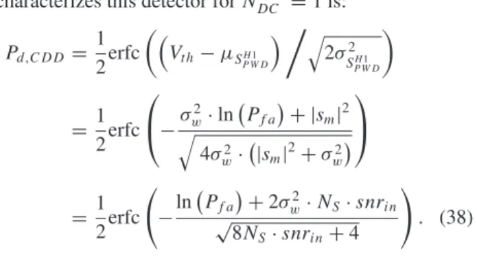
characterizes this detector for NP W DC = 1 is: Pd,CDD = 1 2erfc µ_³ Vt h− µSH1 P W D ´Áq 2σ2 SH1 P W D ¶ = 1₂erfc  − σ2 w· ln¡Pf a¢ + |sm|2 q 4σ2 w·¡|sm|2+ σw2 ¢   = 1 2erfc à −ln¡Pf a¢ + 2σ 2 w· NS· snrin √ 8NS· snrin+ 4 ! . (38) According to (28), the sensitivity loss of a single differential operation as function of Dc, i.e., Ldiff(1, Dc),

can be expressed as: Ldiff(1, Dc) = snrin,req snrin,min = snrin,req· Ns Dc/2 , (39) where snrin,reqin this case is the input SNR required by

the CDD detection scheme to achieve the working point specified by Dc. This required input SNR can be directly

obtained by solving (38) for any pair (Pd, Pf a), but it

should be noted that this expression is based on the Gaussian approximation under H1, which was seen not to

be entirely accurate. Another option is simply to consider the Gaussian and Laplace terms independent, in which case a normal-Laplace random variable is obtained [29]. The expression that characterizes this detector under this assumption is shown in Appendix B. The accuracy of these two approximations of Pd,CDDcan be assessed by

comparing the predicted Pd from (38) and (55) with the

results obtained from the simulation. This comparison is shown in Fig. 9 for the acquisition of a GPS C/A signal, sampled at twice the chip rate (Ns= 2046), Pf a= 10−5,

and 1fd,k= 1ζ = 0. As expected, none of the

approximations represents an entirely accurate prediction of the detector performance. In fact, the predicted performances according to both approximations are almost coincident, from which it can be concluded that the

Fig. 10. Sensitivity loss due to differential operation—theory, simulation, and approximation.

oddity of the differential detector behavior is mostly due to the dependence between the two stochastic terms under analysis.

Fig. 10 shows Ldiff(1, Dc) calculated through (39)

using the snrin,reqvalues for the approximations and

simulation values shown in Fig. 9. All curves are expressed as function of Dc/2. Although the difference

between the approximations and simulation loss values is not considerable, the profile exhibited is significantly different. This fact complicates the proposal of an expression for Ldiff(1, Dc) based on the theoretical loss

curves that is consistent at both high and low SNR values. The issue is with the sensitivity loss formula and not with the metric PDF approximation, meaning that even with a good model of the PWD distribution, it is difficult to obtain a closed formula of the sensitivity loss Ldiff(NDC, Dc).

Therefore, the simulation-derived loss curve is considered. The theoretical analysis, nevertheless, is useful to validate the simulation results. Several different models can be employed in an attempt to approximate the simulation points of Ldiff(1, Dc) shown in Fig. 10. Although various

approximations of different orders of 1/(Dc/2) offer a

good fit in the SNR area under consideration in the figure, their behavior at high and, especially, low SNR values makes them unsuitable for the approximation sought. One approximation that closely matches the simulation results in the SNR range under consideration and that is

consistent for both low and high SNR values is: Ldiff(1, Dc) ≃ 1 + 0.2 Dc/2+ 0.45 3 √ Dc/2 . (40)

This curve is also shown in Fig. 10, where its accuracy in predicting the sensitivity loss induced by one

differential operation is verified. In order to generalize this loss formula to any number of differential operations Ldiff(NDC, Dc), it suffices to note that the SNR at the

correlation output of the CD is written as Dc/NC or, for

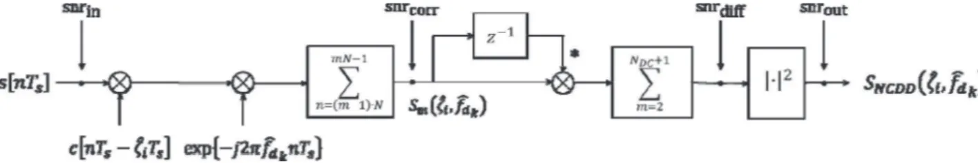
Fig. 11. NCDD block diagram and SNR measuring points.

then be rewritten as:

Ldiff(NDC, Dc) ≃ 1 +0.2 · (N DC+ 1) Dc +0.45 · 3 √ (NDC+ 1) 3 √ Dc . (41) This formula expresses the sensitivity loss incurred by a number NDCof differential integrations (employing

NDC+ 1 coherent outputs) and a receiver working point

specified by Dc(Pd, Pf a) with respect to the coherent

operation. It should be noted that this simple passage from (40) to (41) does not actually take into account the dependence between the consecutive differential outputs. Nevertheless, as it will be seen further, it still seems to be a good approximation of the actual loss experienced by the NCDD.

C. Sensitivity Loss of the NCDD

After characterizing the loss of differential integration, we now extend the analysis to the NCDD loss LN CDD,

which, according to the block diagram shown in Fig. 11, is a combination of both differential integration and squaring loss. According to the procedure previously described, the NCDD sensitivity loss is defined as the additional input SNR required by this detector with respect to the input SNR required by the coherent detection scheme to achieve a similar target working point. The sensitivity gain of the NCDD scheme having Nccoherent outputs available is

then expressed as follows (Dcis omitted in the loss

formulas for simplicity of notation and all the terms are in dB):

GN CDD(Nc) = Gcoh(Nc) − LN CDD(Nc)

= Gcoh(NC) −¡Ldiff(NDC) + Lsq

¢ = GSLD(NC) − Ldiff(NDC) . (42)

This way, we can directly relate the sensitivity gain of the NCDD with that of the SLD by Ldiff(NDC). This will

be particularly useful in the comparison of the NCDD and NCD because the sensitivity loss formula proposed in [31] for the latter, i.e., (47), is also related to the SLD. It should be noted that, even if Ldiff(NDC) was obtained for the

CDD scheme by concentrating all the signal power in the real branch of the correlation output, it expresses the sensitivity loss of the differential operation as function of

the SNR of the coherent output and is independent of its phase. This way, it can be directly applied in (42).

It then suffices to express the differential operation loss as function of the SNR prior to the phase-removal operation snrdiff in Fig. 11. This can be done by recurring

to the squaring loss formula: Lsq=

snrdiff

snrout ≃

1 +√1 + 9.2/snrout

2 , (43) where snrout is the SNR at the output of the NCDD as

shown in Fig. 11. Given that all the loss formulas have been developed with respect to the CD, it then follows that snrout = Dcand therefore:

Lsq = snrdiff snrout = snrdiff Dc ≃ 1 +√1 + 9.2/Dc 2 ⇔ snrdiff ≃ Dc·1 + √ 1 + 9.2/Dc 2 . (44) The sensitivity loss of the NCDD with respect to SLD is finally given by:

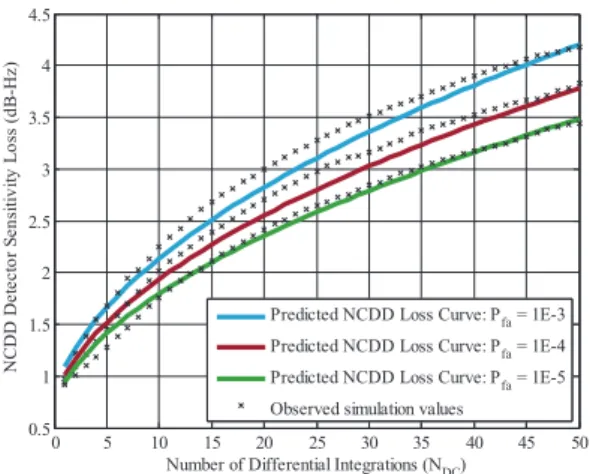
Ldiff(NDC) ≃ 1 +0.2 · (N DC+ 1) snrdiff +0.45 · 3 √ (NDC+ 1) 3 √_snr diff . (45) The accuracy of this formula can be assessed by comparing the predicted and observed sensitivity losses obtained through simulations. Defining a target Pd= 0.9,

the predicted and observed sensitivity loss of the NCDD detection scheme with respect to the SLD in the

acquisition of a GPS L1 C/A signal (Ns = 2046) is shown

in Fig. 12 for three different values of Pf a. From this

figure, it can be seen that there is a very close match between the observed and expected loss profiles for this detector. In fact, the prediction is accurate to within ±0.3 dB in the interval presented for each of the three Pf a

values considered. An example of the accuracy of this formula is shown in Fig. 12 for NDC= 20. It can be

noticed from this figure that the predicted NCDD sensitivity loss at (Pd, Pf a) = (0.9, 10−5) with respect to

SLD is very close to the actual value. For NDCbetween 50

and 100, the maximum error is still within ±0.5 dB. D. Applications of the NCDD Sensitivity Loss Formula

One of the applications of the proposed formula is for characterizing the detection performance of the NCDD.

Fig. 12. Predicted and observed losses for the NCDD scheme with respect to SLD as function of NDCand Pfafor Pd= 0.9.

Fig. 13. Illustration of NCDD sensitivity loss with respect to SLD for NDC= 20 and accuracy of loss formula.

We can use this formula to construct the sensitivity curve of the detector using as reference the curve of the SLD given by (25), as was done in Fig. 13. The comparison between the simulated and predicted detector performance for the scenarios of Table I is plotted in Fig. 14. From this figure, it can be seen that the NCDD sensitivity prediction curve is also accurate when a nonzero Doppler offset is accounted for in the curves of scenarios S2 and S3. More details on the use of this formula for a nonzero Doppler offset are given in sub-Section VB.

Another application of this formula is in the estimation of the number of differential integrations required for the acquisition of a GPS L1 C/A signal at a given input C/N0.

Fig. 15 shows this estimation for three different values of coherent integrations. Having obtained a loss formula capable of quickly providing an estimation of the NCDD’s performance, it is now of interest to compare this detector with its noncoherent counterpart. This analysis is carried in the next section.

Fig. 14. Comparison between simulated and theoretical results for NCDD for simulation scenarios of Table I.

Fig. 15. Number of differential integrations required for NCDD to achieve detection at (Pd, Pf a) = (0.9, 10−5) as function of coherent

integration time and input C/N0.

V. DIFFERENTIAL AND NONCOHERENT DETECTION SCHEMES COMPARISON

The performance comparison of differential and noncoherent detection schemes has been the subject of several studies in recent years [8, 18–21], but to the authors’ best knowledge, the first formal comparison between the NCDD and the NCD is found in [22], based on (45). In this section, the results from [22] are reviewed and extended by evaluating the sensitivity loss of each detector for a nonzero Doppler offset.

A. NCDD and NCD Sensitivity Loss in the Absence of Doppler

The detection metric for the NCD is defined as: SN CD ¡ ˆζi, ˆfdk¢ = NN C X m=1 ¯ ¯Sm ¡ ˆζi, ˆfdk ¢¯ ¯ 2 , (46)

where NN C= NC is the number of noncoherently

accumulated correlation outputs. The sensitivity loss of the NCD LN CDwith respect to the SLD is given in [1, 31]

Fig. 16. Sensitivity loss of NCDD and NCD with respect to SLD for 1fd,k= 0 and NN C= NDC+ 1 ∈ [2, 50] (leftmost point corresponding

to NN C= 2 and rightmost one to NN C= 50).

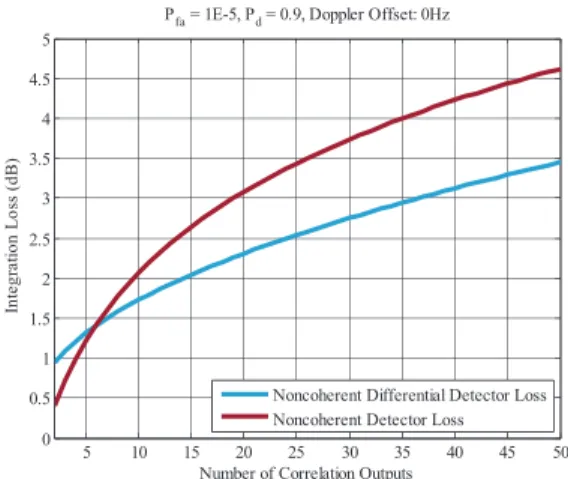
Fig. 17. Sensitivity loss of NCDD and NCD with respect to SLD as function of number of correlation outputs for 1fd,k= 0 and

(Pd, Pf a) = (0.9, 10−5).

as an extension of the squaring loss formula in (34): LN CD(NN C) = 1 +

√

1 + 9.2 · NN C/Dc

1 +√1 + 9.2/Dc

. (47) If the Doppler offset is small enough for its effect on the coherent integration output to be disregarded, a direct comparison between the two loss formulas, (45) and (47), can be used to compare the relative performance of the detectors. In Fig. 16, the losses that would be observed by each scheme with respect to the SLD for three different working points are presented. The number of available code periods is varied from 2 to 50 to obtain the curves shown. According to Fig. 16, for a low number of differential integrations, the combined effect of the differential and squaring loss leads to an inferior

performance of the NCDD with respect to the NCD. This can also be seen in Fig. 17 where the curves for the sensitivity loss of each detector are shown for

(Pd, Pf a) = (0.9, 10−5). As the predictions from both loss

formulas are not exact, conclusions about the precise crossing point should not be taken from these plots. In any

case, it is safe to state that for the acquisition of weak signals, requiring a high number of postcoherent accumulations, the differential detector is a preferable choice.

The effect of the inferior sensitivity loss of the NCDD with respect to the NCD for the acquisition of weak signals is reflected in the acquisition time that each detector needs to achieve the required degree of

confidence in the detection of a given signal with a certain power. In the detection of the presence of signal, the allocation of the signal integration time between the coherent and postcoherent strategy involves a trade-off between sensitivity and complexity. The ultimate practical restriction to the increase of the coherent integration time (considering no navigation data bit influence or dynamics and clock instability effects) is the number of frequency grid points Nfd to be evaluated in the acquisition process.

The usual practice is to define a maximum allowable frequency attenuation for the coherent output that should not be exceeded, resulting in a rule such as [1]:

Nfd = 1Fd δfd = 1Fd x/Tcoh = T coh 1Fd x ,

where 1Fdis the width of the Doppler frequency search

space (typically around 10 kHz), δfdis the frequency grid

resolution (not to be confused with 1fd, the residual

frequency estimation error as defined in Section II), and x is the coefficient resulting from the maximum desired amplitude attenuation [1]: Lδf,max= sinc ³ Tcoh· δfd ± 2 ´ ⇔ δfd = x Tcoh • Lδf,max,dB= 0.5 dB ⇒ x = 1/2 • Lδf,max,dB= 1.9 dB ⇒ x = 1

This way, even if the maximum integration gain is obtained through the increase of the coherent integration time, it directly affects the acquisition process complexity (number of operations required). As an example, we consider a total signal observation time of 20 ms. The highest sensitivity gain possible corresponds to coherently integrating throughout the 20 code periods, i.e.,

Gcoh,dB(20) = 10log10(20) = 13dB.

The other alternatives imply trading off the coherent and postcoherent integration gains according to the equations (values in dB):

GN CD(NN C) = Gcoh(NC) − LN CD(NN C) ,

GN CDD(NDC) = Gcoh(NC) − LN CDD(NDC) .

In Table II, the number of correlator outputs required for each different postcoherent integration strategy to achieve the 13-dB gain for a working point of (Pd, Pf a) = (0.9, 10−5) and for different number of

coherent integrations is shown. The number of frequency grid points is calculated for a grid employing

TABLE II

Integration Strategies Comparison

Correlation Outputs Required Integration Time (ms) Frequency Grid Points NCD NCDD 1 10 64 40 2 20 21 16 4 40 8 7 5 50 6 6 10 100 3 3 20 200 – –

Fig. 18. Sensitivity loss of NCDD and NCD with respect to SLD for 1fd,k= 500 Hz and NN C= NDC+ 1 ∈ [2, 50] (leftmost point

corresponding to NN C= 2 and rightmost one to NN C= 50).

δfd= 1/Tcoh. Naturally, the strategy requiring the shortest

observation time is the one employing the longest coherent integration time. It can also be seen that the performance of the NCDD and NCD schemes become very similar when low postcoherent integration gains are sought. The preferable solution from the ones presented in the table should be found as a compromise between integration time and complexity.

B. NCDD and NCD Sensitivity Loss in the Presence of Doppler

In the presence of a nonzero and stationary Doppler offset, the coherent processing output is affected by the sinc function, as in (6). This means that the SNR at the coherent-processing output will be less than what would be expected for a zero Doppler offset [3, 34]. This way, the effective coherent output SNR, i.e., snrcoh,eff, is given by:

snrcoh,eff = snrcoh· sinc2¡1fd,k· NTs¢ < snrcoh,1fd,k=0,

This extra attenuation in the coherent processing is translated into (44) and (47) as an increase of Dcby

1/sinc2_(1f

d,k· NTs). The comparison for a Doppler

offset of 500 Hz (typically middle of a frequency bin for one coherent integration) is shown in Fig. 18. Although in this figure it can be seen that the crossing point between the NCD and NCDD sensitivity losses occurs at a higher

Fig. 19. Sensitivity loss of NCDD and NCD with respect to SLD as function of number of correlation outputs for 1fd,k= 500 Hz and

(Pd, Pf a) = (0.9, 10−5).

loss value, this crossing occurs in fact for a lower number of accumulations, comparing Figs. 17 and 19. According to these plots, it can be seen that the NCDD remains as the most suitable detector for the acquisition of weak signals. VI. REAL DATA PROCESSING

The validation of the theoretical analysis described in Sections III and IV as well as the comparison between the differential and noncoherent detectors in Section V have been carried using simulated data. In this section, the performance of the NCDD and NCD is assessed with real GPS L1 C/A signals collected at the ISAE, Toulouse. The data acquisition was carried with a NordNav R30 receiver operating at a sampling frequency of 16.4 MHz.

The focus of this work is in the acquisition of weak signals; however, the reception of such signals is unpredictable, and their actual signal power difficult to assess. This way, an alternative approach is followed in which a strong signal is identified and then corrupted with an extra Gaussian noise component. For this purpose, it is essential to demonstrate that the noise environment is effectively Gaussian. As the signal provided by the NordNav R30 receiver is already digitized, this can be achieved by analyzing the noise distribution at the output of correlation when testing the presence of an absent pseudorandom noise (PRN) code, which, according to (5) enables us to estimate the input signal variance. The result of this analysis is shown in Fig. 20. From the histogram shown in this figure, the Gaussian nature of the

environment noise is well remarked. It should be noted that this Gaussian feature was verified in data collections also in deep urban scenarios, e.g., the city center of Toulouse. This validates the methodology employed for the emulation of weak signals and allows testing the algorithms under a wide range of signal strengths.

Two types of analysis are carried out. First, the detectors are compared employing data blocks of fixed size, and their sensitivity curve is drawn. In the second analysis, a fixed attenuation is imposed, and the detectors’

Fig. 20. Noise-only correlation output histogram.

detection rate is plotted as function of the number of available code periods. The Doppler search grid considered in the following examples spans from –5 to 5 kHz, and the frequency resolution in every case considered is 1/Tcoh. For each analysis, a mean of 1 false

alarm per 100 detections is fixed, so the detection thresholds are set by running the detectors for 100 independent data blocks extracted from the short

collection time while testing a nonpresent PRN code. The detectors are then run for these same 100 blocks using the PRN code of the strong signal previously identified. This procedure is repeated for each C/N0point shown in the

plots.

A. Detectors Sensitivity Comparison

The first comparison of the performance of the NCDD and NCD in real data acquisition is performed employing a coherent integration time of 1 ms and 2, 5, and 10 correlation outputs. The signal C/N0is varied as shown in

the plots of Fig. 21. In these plots, it is clear that the NCDD becomes more effective than NCD as the input signal C/N0decreases and, consequently, a longer signal

observation time is required for reliable signal detection. It should be noted that in this analysis no methods for attempting compensation of data bit transition were applied, so in several data blocks, the change in data bit value is encountered. Given the long data bit duration for the GPS L1 C/A signal with respect to its code period, the data bit transition affects both detectors nearly in the same way, even if noncoherent integration is naturally more robust. Nevertheless, the data bit transition issue requires further attention in modern GNSS signals, e.g., Galileo E1, in which the navigation data period is similar to the spreading code period.

B. Weak Signal Acquisition

To show how detection of weak signals is achieved with the different detectors, a signal at an average C/N0of

33 dB-Hz is emulated by adding extra noise to the real signal. The attenuated signal is then attempted to be

Fig. 21. NCDD and NCD sensitivity comparison in acquisition of real signals using 2, 5, and 10 correlation outputs and 1-ms coherent

integration.

acquired with the SLD, NCD, and NCDD. The detection rate verified for each detector is shown in Fig. 22 as a function of the number of code periods integrated. From this plot, it can be seen that this signal can be reliably acquired with any of the three detectors, provided the number of code periods to be integrated is sufficiently high. While the SLD is the best performing one, its

Fig. 22. NCDD, NCD, and SLD sensitivity comparison in acquisition of emulated signal at 33 dB-Hz using 2 to 10 correlation outputs.

complexity of execution is considerably higher than the other two detectors, employing only 1-ms coherent integration and consequently presenting a less stringent requirement on the frequency grid resolution. Also, here, the superior performance of the NCDD with respect to the NCD is observed.

VII. CONCLUSION

In this paper, the performance of post-CDDs in the acquisition of weak GNSS signals was studied. First, we characterized statistically the PWD. Under the noise-only hypothesis, we made use of the fact that the output of pair-wise differential integration corresponds to a sum of independent Laplace random variables to propose a new expression for its characterization. Under the assumption that both signal and noise are present, it was shown that the approximation of the output of this detector by a Gaussian random variable matches closely its true distribution, and an expression for its probability of detection was derived. Given the complexity of following a similar procedure for the NCDD, we instead characterized this detector through its sensitivity loss with respect to the SLD. Firstly, the methodology to characterize a detector in this way was described, and subsequently a formula for assessing the sensitivity loss of the NCDD (combining both differential and squaring losses) with respect to the SLD was

proposed. The theoretical results were validated by simulations, showing that this is a valid approach to follow in such cases when the statistical analysis of the detectors is overly complex.

The results obtained enabled the comparison of the NCDD and NCD, allowing a decision on the most adequate integration strategy for achieving a predefined sensitivity level. It was confirmed that differential integration is in fact preferable to noncoherent integration in the acquisition of weak signals. The theoretical conclusions were confirmed with the acquisition of real GPS L1 C/A signals, highlighting the potential of the NCDD in weak signal acquisition.

APPENDIX A

Under H0, the differential operation output, YH0, is

expressed as: YH0 = wm· w∗_m−1= ³ w_mIwI_{m−1+ wm}Qw_m−1Q ´ + j³w_mQw_m−1I _{− w}Q_m−1wI_m´_{= YH0}I _{+ j YH0}Q. (48) The Y_H0I term can be rewritten as:

Y_H0I _{= wm}IwI_{m−1+ wm}Qw_m−1Q = σw2/2 ·£¡U 2 1+ U 2 3¢ − ¡U 2 2 + U 2 4 ¢¤ = σw2/2 · [x1− x2] , (49)

where all the Unterms are normal-distributed with zero

mean and variance 1: U1=¡wIm+ w I m−1¢ ±√2σw, U2=¡wIm− w I m−1¢ ±√2σw, U3= ³ wQ_{m+ w}Q_m−1´±√2σw, U4= ³ wQ_{m− w}Q_m−1´±√2σw, (50) and, consequently, both x1and x2are independent χ2

random variables with two degrees of freedom [27]. From [35], the distribution of the subtraction of two independent random variables is given by:

fZ(z) =                ∞ Z 0 fX1(z + x2)fX2(x2) dx2, z ≥ 0 ∞ Z −z fX1(z + x2) fX2(x2) dx2, z <0 (51)

where z = x1− x2, and fX1(x1) and fX2(x2) are the PDFs

of x1and x2, respectively, i.e., [35]:

fX(x) =

xn/2−1

2n/2_{· Ŵ (n/2 )}e

−x/2₌ e−x/2

2 , x ≥ 0 (52) with n = 2 the number of degrees of freedom of the χ2

distribution for both x1and x2. This way, fZ(z) can be

easily rewritten as: fZ(z) = (₁ 4 · e−z/2, z ≥ 0 1 4· e z/2_{, z <0} = 1 4· e −|z|/2 ₍₅₃₎

which corresponds to a Laplace distribution of zero mean and diversity or scale parameter l equal to 2 [27]. From this same reference, it comes that the variance of the Laplace distribution is 2l2. Thus, the variance of c · Laplace(l) is then c2

· 2l2= 2l′2, implying that: σ_w2/2 · Laplace (l) = Laplace¡σ2

w/2 · l¢ ,

resulting finally in Y_H0I _{∼ Laplace(σw}2). The same reasoning can be followed to demonstrate that Y_H0Q _{∼ Laplace(σ}2

w) by simply defining a normal random

variable x = −wQmand analyzing the distribution of

wQ

APPENDIX B

Given two independent random variables Z and W , such that Z ∼ N(µ, σ2

) and W ∼ Laplace(l), their sum Y = Z + W results in a normal-Laplace distribution whose PDF and CDF are given by [29]:

fY(y) = φ(γ ) 2l · [R (σ/l − γ ) + R (σ/l + γ )] , (54) FY(y) = 8 (γ ) − φ (γ ) · R(σ/l_{− γ ) + R (σ/}l_{+ γ )} 2 , (55) with γ = (y − µ)/σ , 8(·) and φ(·) the CDF and PDF functions of a standard normal random variable, respectively, and R(·) the Mills ratio, defined as [29]:

R_{(z) =} 8

c_(z)

φ(z) =

1 − 8 (z)

φ(z) . (56) Given a threshold Vt h, the tail probability of Y ,

equivalent to Pd in detection of a signal distributed

according to fY(y), is:

Pd = 1 − FY(Vt h) . (57)

This equation can be employed in the characterization of the output of the CDD under H1, considering the Gaussian

and Laplace noise terms to be independent. For the case of a single differential operation, the terms in (55) and (57) are given by:

l = σ2 w, µ = µSH1 P W D ≃ |sm| 2 , σ2_{= var©ℜ ©w}Y,mªª ≃ 2σw2· |sm|2, Vt h= −σw2 · ln¡Pf a¢ . ACKNOWLEDGMENT

The authors would like to thank Prof. Nesreen Ziedan for her contribution to this work.

REFERENCES [1] Tsui, J. B.-Y.

Fundamentals of Global Positioning System Receivers: A Software Approach(2nd ed.). New York, NY: John Wiley & Sons, Dec. 2004.

[2] Borre, K., Akos, D. M., Bertelsen, N., Rinder, P., and Jensen, S. H.

A Software-Defined GPS and Galileo Receiver—A Single-Frequency Approach. Boston, MA: Birkh¨auser, Nov. 2006.

[3] Misra, P., and Enge, P.

Global Positioning System: Signals, Measurements and Performance. Lincoln, MA: Ganga-Jamuna Press, 2001.

[4] Watson, R., Lachapelle, G., Klukas, R., Turunen, S., Pietil¨a, S., and Halivaara, I.

Investigating GPS signals indoors with extreme high-sensitivity detection techniques.

Journal of the Institute of Navigation, 52, 4 (2005–2006), 199–214.

[5] Kishimoto, N., Vayrus, J. and Weill, L. R.

An ultra-sensitive software GPS receiver for timing and positioning.

Presented at the Proceedings of ION GNSS 2010, Portland, OR, Sep. 21–24, 2010.

[6] Sahmoudi, M., and Landry, R., Jr.

A nonlinear filtering approach for robust multi-GNSS RTK positioning in presence of multipath and ionospheric delays.

IEEE Journal of Selected Topics in Signal Processing, 3, 5 (Oct. 2009), 764–776.

[7] van Diggelen, F.

A-GPS: Assisted GPS, GNSS, and SBAS. Norwood, MA: Artech House, Mar. 2009.

[8] Yang, C., Miller, M., Blasch, E., and Nguyen, T. Comparative study of coherent, non-coherent, and semi-coherent integration schemes for GNSS receivers. Presented at the Proceedings of ION GNSS 2007, Cambridge, MA, Sep. 25–28, 2007.

[9] Pany, T., Riedl, B., Winkel, J., W¨orz, T., Schweikert, R., Niedermeier, H., Lagrasta, S., Lopez-Risue˜no, G., and Jim´enez-Ba˜nos, D.

Coherent integration time: The longer, the better.

Inside GNSS, 4, 6 (Nov.–Dec. 2009), 52–61. [10] Pany, T., G¨ohler, E., Irsigler, M., and Winkel, J.

On the state-of-the-art of real-time GNSS signal acquisition—A comparison of time and frequency domain methods.

Presented at the Proceedings of the International Conference

on Indoor Positioning and Indoor Navigation, IPIN 2010, Z¨urich, Switzerland, Sep. 15–17, 2010.

[11] Sahmoudi, M., Amin, M., and Landry, R., Jr.

Acquisition of weak GNSS signals using a new block averaging pre-processing.

Presented at the Proceedings of IEEE/ION PLANS 2008, Monterey, CA, May 6–8, 2008.

[12] Borio, D., and Akos, D.

Noncoherent integrations for GNSS detection: Analysis and comparisons.

IEEE Transactions on Aerospace and Electronic Systems, 45, 1 (Jan. 2009), 360–375.

[13] Str¨assle, C., Megnet, D., Mathis, H., and B¨urgi, C. The squaring-loss paradox.

Presented at the Proceedings of ION GNSS 2007, Fort Worth, TX, Sep. 25–28, 2007.

[14] Lank, G., Reed, I., and Pollon, G.

A semicoherent detection and Doppler estimation statistic.

IEEE Transactions on Aerospace and Electronic Systems, 9, 2 (Mar. 1972), 151–165.

[15] Zarrabizadeh, M. H., and Sousa, E. S.

A differentially coherent PN code acquisition receiver for CDMA systems.

IEEE Transactions on Communications, 45, 11 (Nov. 1997), 1456–1465.

[16] Rodriguez, J. A. A., Pany, T., and Eissfeller, B.

A theoretical analysis of acquisition algorithms for indoor positioning.

Presented at the Proceedings of NAVITEC 2004, Noordwijk, The Netherlands, Dec. 8–10, 2004.

[17] Iinati, J., and Pouttu, A.

Differentially coherent code acquisition in Doppler. Presented at the Proceedings of IEEE Vehicular Technology

Conference, Amsterdam, The Netherlands, Sep.19–22, 1999. [18] Villanti, M., Salmi, P., and Corazza, G. E.

Differential post detection integration techniques for robust code acquisition.

IEEE Transactions on Communications, 55, 11 (Nov. 2007), 2172–2183.