DOCTORAT DE L'UNIVERSITÉ DE TOULOUSE
Délivré par :
Institut National Polytechnique de Toulouse (INP Toulouse)
Discipline ou spécialité :
Energétique et Transferts
Présentée et soutenue par :
M. NAJIB BELGACEM le jeudi 14 avril 2016
Titre :
Unité de recherche : Ecole doctorale :
MODELISATION MIXTE CONTINUE - RESEAU DE PORES DES
TRANSFERTS DIPHASIQUES CATHODIQUES D'UNE PILE A
COMBUSTIBLE PEMFC
Mécanique, Energétique, Génie civil, Procédés (MEGeP)
Institut de Mécanique des Fluides de Toulouse (I.M.F.T.)
Directeur(s) de Thèse :
M. MARC PRAT
Rapporteurs :
M. BRUNO AUVITY, POLYTECH NANTES
Mme SOPHIE DIDIERJEAN, UNIVERSITE DE LORRAINE
Membre(s) du jury :
1 M. YANN BULTEL, INP DE GRENOBLE, Président
2 M. JOEL PAUCHET, CEA GRENOBLE, Membre
2
Remerciements
Mes premiers remerciements sont à Marc Prat mon directeur de thèse qui m’a accordé sa confiance. Ses conseils, son suivi et ses aides sont très précieuses durant toute la thèse. Merci beaucoup Joël pour tous les échanges qu’on a eu durant la thèse. Ton regard critique envers mes résultats m’a bien aidé. Tu as allégé les moments difficiles avec ton sens humain. Dominique grand merci pour tous tes aides, ton soutien et tous les échanges.
Samira ne change pas ;), merci pour ton grand humour et tes gâteaux …
Merci Beaucoup Pierre-André, Arnaud, Frèd, Tristan, Yohan, Marie, Inès, Marion.
Emeline merci pour les cafés tous les matins, les sorties mêmes qu’elles n’étaient pas nombreuses.
Je remercie également mes amis qui m’ont bien soutenus: Anis, Meycèn, Mahmoud, Ayoub (Arfaoui et Nouri), Oussama…,un merci spécial à mes amis de Nantes qui ont une place particulière dans mon cœur.
Merci Samir et Brahim.
Merci mes frères Mohamed, Hedi et Taher. Merci Rim et Ibtissèm.
Merci à toutes mes belles sœurs.
3
Re sume
Cette thèse présente une contribution à l’étude des transferts d’eau au sein des piles à combustible de type PEMFC, un aspect clé de cette technologie. Une approche de simulation numérique est développée en couplant un modèle de type réseau de pores dans la couche de diffusion (DM), une approche mixte continue –réseau de pore dans la couche microporeuse (MPL) et une modélisation par compartiments dans la couche active. L’approche développée prend en compte les transferts couplés de chaleur et d’eau via notamment la modélisation des phénomènes de changement de phase dans la DM et la MPL (évaporation et condensation). Dans une première partie, nous étudions le cas où l’eau migre dans l’assemblage MPL-DM directement en phase liquide. L’impact de la variation de pression dans la phase gazeuse sur la distribution de la phase liquide est étudié. L’épaisseur optimale de la MPL est également étudiée. Dans une seconde partie, nous étudions des situations où l’eau se forme par condensation dans la couche de diffusion. Nous étudions tout d’abord l’impact des propriétés de la couche de diffusion et de la MPL sur le diagramme de condensation. Ensuite nous analysons l’impact de la formation de l’eau liquide sur la distribution de courant locale. Enfin, l’impact de la mouillabilité sur les figures de condensation est étudié. Cette dernière étude est vue comme un premier pas vers l’étude des mécanismes de dégradation dans le régime de condensation.
4
Contenu
Partie I
:Scénario injection
Chapitre 1 : Influence of transverse gas pressure gradient on liquid water invasion in GDL Chapitre 2 : Liquid invasion from multiple inlet sources and optimal gas access in a two-layer thin porous medium
Partie II
Scénario condensation
Chapitre 3 ModelingChapitre 4 : Calage et validation des modèles
Chapitre 5 : Gas diffusion layer condensation diagram in proton exchange membrane fuel cells
Chapitre 6:Impact of liquid water formation on the current local distribution at the cathode gas diffusion layer-catalyst layer interface in proton exchange membrane fuel cells Chapitre 7 : Impact of the wettability on condensation pattern in the gas diffusion layer Conclusion et perspectives
5
Introduction
Les besoins mondiaux en énergie ne cessent d’augmenter. À ce jour, ces besoins sont couverts principalement par les énergies fossiles. Ces sources d’énergie ne sont pas renouvelables et elles contribuent pour une grande part au problème du réchauffement climatique.
Dans ce contexte, le transport figure parmi les secteurs les plus consommateurs en énergie et beaucoup de travaux sont entrepris pour trouver une alternative aux moteurs thermiques qui soit fiable et économiquement compétitive. Pour ce qui est de l’automobile par exemple, les efforts se concentrent autour de motorisations d’origine électrique. Deux principales technologies sont mis en œuvre : les systèmes utilisant un système de stockage de l’électricité dans des batteries et ceux s’appuyant sur la technologie des piles à combustible (PAC) basse température. Une pile à combustible est un système de conversion de l'énergie chimique en énergie électrique, offrant une bonne solution au problème de stockage de l'énergie. Les PAC sont l’objet d’intenses recherches et développements à travers le monde, notamment en Amérique du nord, au Japon et bien sûr en Europe. Les efforts actuels visent notamment à améliorer les performances, la durée de vie de ces systèmes et en minimiser le cout. Ces efforts visent aussi à étendre l’applicabilité des PAC. Pour ne citer qu’un exemple hors de l’automobile, MyFc est une société d'innovation suédoise qui développe et industrialise des solutions pour alimenter les appareils électroniques portatifs. Un de ces produits le PowerTrekk est un chargeur à pile à combustible à prix abordable (199 €) compatible avec de nombreux objets nomades comme les tablettes, les téléphones portables, les appareils photos, ….
Figure 1 : PowerTrekk : chargeur à pile à combustible
Dans le secteur transport, Toyota a commercialisé très récemment une voiture fonctionnant avec la technologie PAC : la Mirai . Celle-ci est commercialisée depuis décembre 2015 au Japon (avec une commercialisation en France prévue en 2017). Son cout hors taxes est estimé à 66000 € en Allemagne. Son énergie est produite par une pile à combustible à membrane échangeuse de proton (PEMFC pour son acronyme anglais) capable de produire une
6
puissance maximal de 114kW pour alimenter une moteur électrique de puissance 113 kW (154 ch DIN).
Figure 2 : Toyota Mirai
Elle a une autonomie de 500Km et se ravitaille en 3 minutes comme une voiture à essence. Elle contient notamment deux réservoirs d’hydrogène stockés sous une pression de 700 bars. Pour plus des détails voir le site internet suivant :
http://www.moteurnature.com/actu/2014/toyota-mirai-hydrogene-pile-a-combustible.php
La Mirai est un exemple de voitures fonctionnement purement à l’hydrogène. Il existe aussi des voitures hybrides électrique/hydrogène. Par exemple, l’utilitaire Renaud Kongo ZE H2 est une voiture électrique qui contient une pile à combustible. Celle-ci est utilisée pour recharger la batterie, ce qui permet d’augmenter l’autonomie du véhicule.
Dans ce contexte, cette thèse a pour objet les PEMFC. Elle a été financée par un projet européen from the European Union’s Seventh Framework Programme (FP7/ 2007-2013) for the Fuel Cells and Hydrogen Joint Technology Initiative. Il s’agit du projet IMPACT “IMPACT— Improved Lifetime of Automotive Application Fuel Cells with ultra-low Pt-loading” (grant agreement n°303452).
Une PEMFC est un dispositif électrochimique produisant du courant pour une tension donnée. Le schéma d’une cellule élémentaire et de ses principales couches constitutives est présenté sur la Figure 2. Dans les applications, les cellules sont mises en série (pour augmenter la tension) ou en parallèle (pour augmenter la densité de courant) dans un assemblage appelé stack (Fig.3). Chaque cellule est alimentée par un système de canaux en hydrogène (coté anode) et en air (coté cathode). Les réactions chimiques se produisent dans les couches catalytiques (couches actives de la Fig.3). Des couches additionnelles appelées couches de diffusion (GDL ou gas diffusion layers) sont placées entre les couches actives et les plaques portant les canaux d’alimentation en hydrogène et air. Les GDLs ont pour but d’homogénéiser les flux électriques, de chaleur et de masse entre les couches actives et la zone des canaux.
7
Figure 3 : Cellules assemblées en stack (à gauche). La figure de droite montre les différentes couches constitutives d’une cellule.
Le rôle de la GDL est de garantir le transport des charges (électrons) (par sa structure solide en carbone), le transfert des gaz (dans les pores), et de contrôler l’eau liquide dans le MEA (traitement hydrophobe).
Elle a ainsi un rôle très important sur les performances des PEMFC (Williams et al, 2004; Park et al., 2012). Des expériences montrent que la MPL a un rôle également important sur les performances (Park et al., 2006; Karan et al., 2007).
La GDL est une composante clé pour assurer une bonne gestion de l'eau liquide dans le MEA ((Mathias et al., 2003; Wood, 2006; Wood and Borup, 2010; Li et al., 2008). Elle joue ainsi un rôle crucial sur l’équilibre : maintenir une bonne hydratation d’ionomer (pour avoir une bonne conductivité protonique de la membrane) sans avoir produit beaucoup d’eau liquide qui bloquerait le passage des réactifs vers la CL.
Ainsi, il s’avère très important de mieux comprendre le transport de l’eau liquide dans la GDL, et spécialement de pouvoir analyser plus précisément l’écoulement diphasique et la diffusion des gaz dans la GDL.
La GDL est composé d’un support de diffusion DM (Diffusion Medium) et d’une couche microporeuse MPL( Micro Porous Layer) (figure 4).
Le DM est une structure poreuse constituée de fibres de carbone (8 - 10 µm de diamètre), avec parfois un liant. Un traitement hydrophobe (généralement à base de PTFE) est introduit dans le DM en général par imprégnation.
La MPL est également une structure poreuse, mais à base de noir de carbone (CB) avec un agent hydrophobe (en général également PTFE) qui assure la résistance mécanique. Elle est déposée sur le DM et selon les propriétés du DM (Par exemple sa mouillabilité et sa porosité) et de la MPL (Par exemple sa viscosité), la MPL peut pénétrer ou non à l'intérieur du DM (pas de pénétration de la MPL sur la figure 4). La MPL peut aussi avoir des fissures sur sa surface (figure 5).
8
Figure 4 : image SEM d'une GDL avec la MPL a) et le DM (b) (image du CEA); Les fibres de carbone sont en gris
Figure 5: Vue de la surface d'une MPL avec quelques fissures Gestion de l’eau, transfert de chaleur, durabilité
Les problèmes de durabilité constituent sans doute le principal frein à la commercialisation massive de la technologie PEMFC. A titre indicatif, une pile a typiquement une longévité de quelques milliers d’heures si bien qu’il n’est pas possible d’espérer effectuer plus de 100 000 km dans le cas de l’application automobile. C’est particulier gênant lorsqu’il s’agit de l’élément le plus coûteux de la voiture. Ces problèmes de dégradation sont en réalité intiment liés à deux autres aspects clé de cette technologie, la gestion de l’eau et les transferts de chaleur au sein de la pile, que ce soit à l’échelle d’une cellule unique de laboratoire ou à l’échelle d’un stack. La gestion de l’eau est classiquement présentée comme le problème d’assurer une humidification correcte de la membrane (afin d’assurer un bon transport des protons H+ à travers cette membrane) tout en évitant de noyer des GDLs ce qui a pour conséquence de limiter sévèrement l’accès des gaz aux couches actives. Le problème de la gestion de l’eau ne peut en fait être découplé de celui des transferts de chaleur en raison de l’importance des phénomènes de changement de phase liquide-vapeur au sein de la pile. Les transferts de chaleur et notamment les hétérogénéités spatiales de température jouent un rôle clé dans les mécanismes de dégradation, e.g. Nandjou (2015), Abbou (2015) si bien qu’en réalité c’est pour une large part une meilleure compréhension du triptyque transfert d’eau, transfert thermique, dégradation qui doit être développée pour améliorer la technologie PEMFC. µm po reu x Su pp ort de G D L µm po reu x Su pp ort de G D L a) MPL b) DM Carbon Fibers
9
Dans ce contexte et compte tenu du grand nombre de travaux dédiés ces vingt dernières années aux PEMFC, on peut s’étonner que les mécanismes contrôlant les transferts de l’eau au sein d’une cellule, ne soient pas complétement élucidés. Il s’agit là d’un point crucial si l’on veut espérer une stratégie de développement organisée qui aille au-delà des stratégies expérimentales courantes par essais – erreurs dont le défaut essentiel est que très souvent, on se retrouve en incapacité d’expliquer les résultats obtenus faute d’une compréhension suffisante de ce qui se passe au sein de la pile.
Comme noter dans Straubhaar (2015), même le cas des GDL, a priori plus simple compte tenu notamment du fait que les GDLs ne sont pas le siège des réactions électrochimiques et qu’au moins le medium de diffusion (DM) peut être imagé par tomographie X ou par absorption de neutrons, reste un sujet d’études.
Si par exemple, on se limite comme dans Straubhaar (2015) aux études s’appuyant sur des modèles de réseaux de pores (pore network models (PNM)), techniques de modélisation que nous utilisons également dans ce travail, on peut faire le constat suivant. Pratiquement toutes les études avant le travail de Straubhaar (2015), sont basées sur le scenario, défini comme le scénario #1, où l’eau entre en phase liquide dans le GDL depuis la couche active voisine (ce scenario est illustré sur la Fig. 6a)
a) b)
Figure 6: Schémas illustratifs des deux situations de base en ce qui concerne la phase, liquid ou vapeur, sous laquelle l’eau entre dans la GDL depuis la couche active (CL) : a) scenario #1, eau entrant sous forme liquide (en bleu), (b) scenario #2; eau entrant dans la GDL sous forme vapeur (lignes pointillées bleues), (tiré de Straubhaar et al. 2016).
A la différence de tous ces travaux, voir Straubhaar et al. (2016) pour une revue bibliographique, le scenario privilégié dans la thèse de Straubhaar (2015), dit scenario #2 sur la Fig.6b, est un scénario selon lequel l’eau entre dans la GDL sous forme vapeur à l’interface CL – GDL. Selon ce scenario, l’eau liquide peut se former dans la GDL (et en particulier dans le DM) si l’humidité relative dans le canal et la densité de courant sont suffisamment fortes
10
par condensation. A la différence du scenario #1, ce scenario est intimement lié aux transferts thermiques car la condensation est d’autant plus probable que la variation de température est notable à travers la GDL.
Comme montré dans Straubhaar (2015), les simulations réseau de pores du scenario de condensation sont en accord qualitatif avec plusieurs mesures expérimentales et observations in situ, du moins pour une température de fonctionnement classique proche de 80°C.
La présente thèse s’est déroulée en même temps que ce changement de paradigme, i.e. du scénario #1 au scénario #2. Ceci explique que nous avons travaillé à la fois selon les hypothèses du scenario #1 (première partie de la thèse) et du scenario #2 (seconde partie de la thèse) quand il est devenu clair que le scénario de condensation paraissait la façon la plus appropriée de comprendre la formation de l’eau dans la GDL.
Même si il n’y a plus beaucoup de doutes quant à la pertinence du scénario de condensation aux températures assez élevées (i.e. 80°C), il est à noter cependant que la situation n’est pas encore clarifiée aux températures « froides ». Il n’est donc pas du tout à exclure que le scenario # 1 (injection liquide) mérite toujours considération, ne serait-ce que pour les températures froides par exemple.
Dans ce contexte, la thèse est ainsi organisée en deux grandes parties. La première est basée sur le scenario #1. On y discute deux points. Le premier (Chap.1) est dédié à une étude courte sur le possible impact de l’écoulement de la phase gazeuse au sein du DM sur les figures d’invasion. Le second (Chap. 2) est une étude sur le rôle de la MPL sur l’accès de l’oxygène vers la couche active dans le cadre du scenario #1. Ce chapitre correspond à l’article Belgacem et al. (2016).
La deuxième partie est formée de 5 chapitres (Chap. 3-7) est basée sur le scénario de condensation. On présente tout d’abord un modèle couplant les transferts entre la membrane la couche active et la GDL (MPL + DM). Ce modèle a comme originalité de s’appuyer sur une modélisation réseau de pores pour ce qui concerne le DM. Le Chapitre 4 décrit comment les paramètres du modèle du chapitre 3 ont été spécifiés. Les trois chapitres qui suivent sont dédiés à l’exploitation de ce modèle. Le chapitre 5 étudie l’impact de différents paramètres sur le diagramme de condensation (le diagramme de condensation donne en fonction de l’humidité relative dans le canal la densité de courant critique à partir de laquelle l’eau se forme par condensation dans le DM). Le chapitre 6 s’intéresse à l’impact de la formation de l’eau liquide sur la distribution de densité de courant à l’interface couche active – GDL. Le Chapitre 6 donne un aperçu sur l’impact des conditions de mouillabilité sur les distributions de phase liquide et gaz dans le DM lors de la condensation.
Pour tous ces chapitres, on se place à l’échelle dent canal.
Enfin, il est à noter qu’il est souvent question de dégradation dans le modèle du chapitre 2. La simulation de mécanismes de dégradation fait partie des objectifs majeurs du projet européen « Impact » qui a financé cette thèse. Ces simulations sont renvoyées à l’après thèse car il n’a pas été possible d’avancer suffisamment sur cette partie dans le cadre de la thèse.
11
Références
S.Abbou, Phénomènes locaux instationnaires dans les piles à combustible à membrane (PEMFC) fonctionnant en mode bouché (dead-end), Thèse Université de Lorraine, (2015). N.Belgacem, T.Agaësse, J. Pauchet, M. Prat, Liquid invasion from multiple inlet sources and optimal gas access in a two-layer thin porous medium, Transport in Porous Media, DOI 10.1007/s11242-016-0630-1 (2016)
F.Nandjou, Local study of temperature distribution in P.E.M fuel cells for automotive applications. Correlation between local temperature and degradations, Ph.D thesis, Grenoble Alpes University, (2015).
B.Straubhaar, Pore network modelling of condensation in gas diffusion layers of PEMFC, Ph.D thesis, Toulouse University (2015)
Straubhaar B., J.Pauchet, M. Prat, Pore network modelling of condensation in gas diffusion layers of proton exchange membrane fuel cells, submitted (2016
12
13
Chapter 1
Influence of transverse gas pressure gradient
on liquid water invasion in GDL
Abstract
In this chapter, we study from pore network simulations the possible impact of transverse gas flow within the diffusion medium (DM) of the GDL at the rib –channel scale on liquid water invasion patterns and oxygen access to the catalyst layer (CL). The study is performed considering scenario #1, that is assuming liquid water enters the DM in liquid phase from the adjacent CL or MPL.
Introduction
1.In this chapter, only the diffusion medium on the cathode side is considered assuming that water enters the DM in liquid phase from the MPL / CL area (scenario #1). We implicitly refer to the serpentine channel configuration on the bipolar plate. Because of the gas pressure drop within the serpentine channel, a total pressure difference exists between two close meanders of the serpentine channel. This induces a gas flow within the DM below the rib from the upstream channel section to the downstream channel section. In this context, the objective is to evaluate the possible impact of the transverse gas flow within the DM on the liquid invasion patterns within the DM. The work is based on pore network (PN) simulations developed in 2D and 3D domains. It must be pointed out that the impact of the transverse gas flow on liquid invasion patterns has not been addressed in the literature, at least the one based on PN simulations. A schematic of the situation investigated is shown in Fig.1.
Figure 1 Schematic of the gas transverse flow between serpentine channel upstream section and downstream section on each side of the rib.
14
Pore network model
2.
The computational domain contains between one to three unit cells (a unit cell at the rib – channel scale typically corresponds to a rib and two half channel sections, or to two half rib and one channel). Examples of unit cell used in the present chapter are depicted in Fig.2 (2D) and Fig.3 (3D).
Figure 2: 2D unit cell with gas pressure boundary conditions.
Figure 3: 3D unit cell with gas pressure boundary conditions
As in several previous works, e.g. Rebai et al. (2009), Ceballos et al. (2011), (2013), the DM is represented as a square network (2D) or a cubic network (3D) of pores interconnected by narrower channels (as illustrated in Fig.4). The distance between two pores (two neighbour intersections in the network) is referred to as the lattice spacing. The lattice spacing is denoted by a. As in Rebai et al. (2009), we took a ≈ 50µm. The size of the computational domain in
15
the in-plane directions in Figs.2 and 3 is L=2mm (this corresponds to the size of the rib plus twice the half channel width).
Figure 4: 2D square network (left) and 3D cubic network (right).
Expressed in lattice spacing units, the network size is therefore 40xl in 2D and 40 x 40 x l in 3D where l refer to the DM thickness.The DM thickness is typically in the range [170 – 400] µm. This amounts to considering networks of size 40 x N with N in the range [4, 8] in 2D
(networks of size 40 x 40 x N in 3D). Therefore, there are 40 pores along an in-plane direction and between 4 to 8 pores in the through-plane direction. The narrower channels between two pores are referred to as throats or bonds. Their sizes, denoted by dt, are randomly distributed over the network according to a given probability density function (p.d.f.) within the range [dtmin, dtmax] with dtmin =20 μm, dtmax =34μm.
Gas pressure computation
3.Compared to previous works considering scenario #1, e.g. Rebai et al. (2009), Ceballos et al. (2011), (2013), the main new feature here lies in the fact that the total gas pressure varies within the DM. The method to compute the pressure field in the gas phase within the pores occupied by the gas phase in the network is somewhat classical, e.g. Gostick et al. (2007). The flow rate qij between two adjacent gas pores i and j is expressed using a Poiseuille like expression as ) P (P g = qij h,ij j i (1)
16
where gh,ij is the hydraulic conductance of the throat between pore i and pore j,
a d g t ij h, 128 4
where μ is the gas viscosity. Then we express the volume conservation at each pore of network (note that the variation of gas density with the pressure is neglected),
0 = ) P (P g j i n j h,ij
(2)Solving numerically Eq.(2) with appropriate boundary conditions yields the gas pressure in each pore occupied by the gas phase pore within the DM.
The pressure boundary conditions are presented in Fig.2 (2D) and Fig.3 (3D). As can be seen, we impose different pressure values on the lateral surfaces of network and at the channel / DM surface. The idea is to take into account the transverse pressure difference resulting from the pressure drop within the serpentine channel. Assuming that the channel upstream is on the left and the channel downstream on the right in Figs. 2 and 3, the highest pressure value P+∆P is imposed on the left lateral edge (2D) or surface (3D) of network whereas a lower pressure P-∆P is imposed along the boundary on the right. The pressure P is imposed at the DM - channel interface. This procedure is straightforwardly extended when more than one unit cell is considered as illustrated in Fig. 5.
Figure 5: Gas pressure boundary conditions in a three cells network.
Liquid water invasion PN algorithm in the presence of a
non-4.uniform gas pressure
According to scenario #1, water is supposed to enter the DM in liquid phase from the DM / MPL or DM / CL interface. The DM is supposed to be perfectly hydrophobic (θ ~ 110 °) and it is widely admitted that the invasion is essentially by capillary forces, i.e. viscous forces can be neglected in the liquid phase, see Rebai et al. (2009) for more details. Under these circumstances, the liquid invasion can be simulated using the classical invasion percolation
17
algorithm, e.g. Wilkinson and Willemsen (1983). An invasion capillary pressure threshold is assigned to each throat as (Laplace’s law),
t g d
pcth 4cos (3)
with g 180 (g is the contact angle measured in the gas phase); γ is the surface tension. Then, the IP algorithm simply consists in invading the network each throat at a time (together with the throat adjacent pore not yet filled with liquid) selecting at each step the throat located on the liquid-gas interface of lowest invasion capillary threshold. This is when the total gas pressure is uniform. When the gas pressure P is not uniform the liquid pressure Pl necessary to invade a throat is given by the equation
t g d
pcth 4cos =P(x,y,z )-Pl(x,y,z) (4)
From Eq.(4), we thus define a throat invasion potential as
cth th P(x,y,z) p
(5)
The algorithm then simply consists in selecting at each step the throat of greatest potential. Naturally, the classical IP invasion rule is recovered when the gas pressure is uniform. Thus here the invasion threshold depends not only on the throat size but also on the gas pressure. The invasion is performed until breakthrough, that is until the liquid phase reaches the channel.
A last point concerns the injection boundary condition at the DM – CL or DM – MPL interface. As pointed out in Ceballos and Prat (2010), the classical boundary condition used in IP simulation is to assume that the pressure in the liquid along this interface is uniform. It was argued in Ceballos and Prat (2010) that such a boundary condition is not adapted to GDL on the grounds that the water is produced through a series of discrete sites in the CL. This led to propose a different boundary condition referred to as a multiple injection boundary condition. With this boundary conditions, a fraction of the injection throats present at the DM inlet (=DM – CL or DM – MPL interface) are considered as injection throats. In what follows we have used a variant of the multiple injection BC combined with the IP invasion rule
18
computed from the potential given by Eq.(50). The procedure was as follows. A number ni of injection throats at the DM inlet is chosen randomly (between 1 and 40 in 2D and 1 and 40x40 in 3D). Then the IP invasion rule was applied starting with the selected ni injection throats.
Estimate of gas pressure difference across the unit cell
5.Wang et al. (2010) presented a series of experimental and numerical studies analyzing velocity and pressure drop within the channel of the bipolar plate. These results are summarized in Table 1.
The cells referred to as 12-11 corresponds to a channel width equal to 1mm, see Wang et al. (2011).The total pressure drop over the plate is 1375 Pa, which corresponds to a pressure drop ∆P = 125 Pa between the two sides of a rib. This pressure variation can be compared to the range of invasion capillary pressure thresholds (Eq.(3)):
max min cth cos 4 cos 4 t g t g d d p =
1688 Pa. Thus, ∆P / pcth ~ 7% which shows that the impact of gas pressure variation is not
negligible (in fact the impact is expected to be greater than estimated here because the range of throats typically selected in the invasion percolation process is narrower than considered here; the narrower throats are actually not invaded).
Note that the gas pressure field is recomputed after each invasion (with no flow rate boundary condition on the liquid throats in contact with the gas phase). Thus the pressure drop increases locally within the network as the network is invaded by the liquid phase. The variations of temperature with the DM are neglected.
19
Simulations
6.
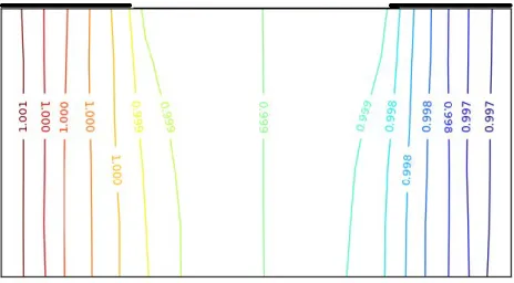
1.1. Gas pressure field structure
Fig. 6 shows the structure of the pressure field in a dry DM. As can be seen the pressure gradients are concentrated below the ribs.
Figure 6: Gas pressure field structure in a dry DM in a transverse cross sect of the unit cell. The gas pressure was made dimensionless using the pressure at the channel – DM surface. Since the gas pressure is greater below the upstream rib and lower below the downstream rib, it is expected from Eq.(5) that the liquid invasion will be easier in the region of the downstream rib where the gas pressure is lower.
1.2. Liquid water invasion patterns
Fig. 7 and Fig.8 show examples of liquid invasion patterns in 2D and 3D unit cell respectively, when the transverse gas pressure difference is varied.
20
Figure 7: Liquid water (in red) invasion patterns for various transverse gas pressure differences in 2D network.
Figure 8: Liquid water (in red) invasion patterns for various transverse gas pressure differences in 3D network.
21
These figures illustrate the impact of the transverse gas pressure variations on the pattern with as expected a preferential invasion of the region below the downstream rib when the transverse gas pressure variation is sufficiently high.
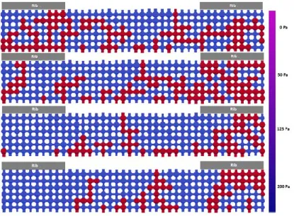
Fig. 9 shows similar results for the 2D computational domain with three unit cells (note that a no gas flow boundary condition is imposed on the right lateral edge of network in this case (this would corresponds to a series of three unit cells with the one the most on the right corresponding to the channel exit).
The displacement of the liquid patterns toward the downstream region is still more marked.
∆P=0
∆P = 50 Pa
∆P=125 Pa
∆P=200 Pa
Figure 9: Liquid water (in red) invasion patterns for various transverse gas pressure differences in 2D three unit cells network.
22
Influence of transverse gas pressure gradient on saturation
7.
The saturation is defined as the volume fraction of the pore space occupied by liquid water. The saturation was computed at the end of invasion. The saturation was actually computed in the three cells depicted in Fig.10 for various transverse gas pressure differences. The results are summarized in Tables 2 and 3. Note that the results presented in Tables 2 and 3 are mean values over 10 realizations of network.
Figure 10: The 3 cells considered for the computation of the saturation.
∆P(Pa) 0 50 125 200
Cell 1 0.16 0.05 0.001 0
Cell 2 0.15 0.13 0.03 0.01
Cell 3 0.156 0.29 0.29 0.2
Table 2: Mean saturation (over 10 network realizations) in the 3 cells in 2D network as a function of transverse gas pressure difference. Note that the indicated pressure difference corresponds to the pressure variation over one cell (the total pressure difference over the three
23
∆P(Pa) 0 50 125 200 Cell 1 0.042 0.005 0 0 Cell 2 0.041 0.02 0.003 0.0002 Cell 3 0.04 0.04 0.032 0.04
Table 3: Mean saturation (over 10 network realizations) in the 3 cells in 3D network as a function of transverse gas pressure difference. Note that the indicated pressure difference corresponds to the pressure variation over one cell (the total pressure difference over the three
cells is therefore three times this value).
Figure 11 shows the through plane mean saturation profiles. It can be seen that the transverse pressure difference has relatively little impact on the saturation in the two rows of pores located next to the CL. This can be understood since the transverse gas pressure difference actually increases locally as the liquid pattern develops since less and less space is available for the gas flow. The impact is quite significant when the liquid approaches breakthrough.
Figure 11: Influence of transverse gas pressure difference on through-plane saturation profiles (3D one cell network). The saturation is a mean saturation over 10 realizations of network.
24
Influence of transverse gas pressure gradient on effective diffusion
8.
coefficient
1.3. Computational method
The effective diffusion coefficient of the DM is computed considering only the diffusion as transport mechanism of the gas components. This is justified by the fact that the Peclet number is smaller than 1. In other terms, the gas flow can have an impact on the liquid invasion pattern but the convective transport of the gas species transport can be neglected.
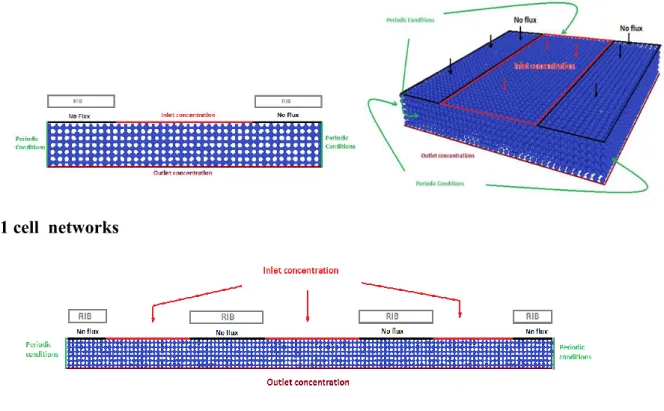
1 cell networks
3 cells network
Figure 12: Boundary conditions for the computation of the diffusive transport in gas phase. The PN computation of the effective diffusion coefficient is described in Gostick et al. (2007). The procedure is analogous to the one used for the computation of the gas pressure field. The diffusive flow rate nij of species A in stagnant species B between two adjacent gas pores i and
25 ) x x ( g = nijA d,ij ln Bjln Bi (6)
where xB,j is species B molar fraction in pore j, and xB,i is species B molar fraction in pore i. gd is the diffusive conductance between the two pores. gd is expressed for a tube of length l and diameter d as l d cD gd,ij AB 2 (7)
where c is the molar density of the mixture and DAB is the binary diffusion coefficient. The diffusive conductance between the two pores is computed as the harmonic average of the conductance of the throat between the two pores and the conductances of half pore i and half pore j, j p t d, pi d, ij d, g g g g , 1 1 1 1 (8)
The next step is to express the mass conservation in each gas pore of network as
0 ln lnx x )= ( g Bj Bi n j d,ij
(9)which leads to a linear system which can be solved with appropriate boundary conditions to obtain the molar fraction of species B in each pore. There is no transport in the pores occupied by liquid.
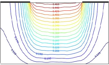
The boundary conditions are summarized in Fig.12 for the various computational domains. Figure 13 below shows two examples of molar fraction fields so obtained in the pore network.
26
one cell 2D network
three cells 2D Network
Figure 13: Examples of A species molar fraction isocontour lines in 1 cell and 3 cells 2D network.
Once the molar fraction is computed, it is easy to determine the diffusive flow rate NA of species A in the through plane direction (we simply sum up the diffusive flow rate in every throat located in a plane perpendicular to the through plane direction). We then express that this diffusive flow rate in the through plane direction must be equal to the macroscopic expression of the diffusive flow rate using Fick’s law,
27 ) x x ( h A cD = N eff n Bj Bi A ln ln (10)
where xB,in and xB,out are the inlet and outlet mole fractions of stagnant species B, h is the
thickness of the DM and An is the cross-section area of the network in the in plane directions
(An= (40-1)x(40-1)a2 in the 40 x 40 x l network). This enables one to determine the effective
through plane diffusive coefficient Deff from Eq.(10).
1.4. Impact of ∆P on effective through plane diffusion coefficient
To show the effect of transverse pressure gradient on effective diffusion coefficient in one cell network, we proceed as follows:
- a transverse pressure difference is imposed.
- Molar fraction boundary conditions are imposed (as depicted in Fig.12).
- Start liquid invasion and at every step of invasion compute overall saturation and effective diffusion coefficient.
Figure 14 shows the variation of the effective diffusion coefficient as a function of overall saturation for different values of transverse pressure difference.
Figure 14: Effective diffusion coefficient as a function of overall saturation for different value of transverse gas pressure difference in a one cell 2D network (results are mean values over
10 realizations of network). 0,00 0,20 0,40 0,60 0,80 1,00 1,20 0,00 0,05 0,10 0,15 0,20 0,25 0,30 De ff( S) /De ff( 0) Saturation DeltaP = 0 Pa DeltaP = 100 Pa DeltaP = 400Pa
28
As can be seen the effective diffusion coefficient increases for a given overall saturation with the transverse gas pressure difference ∆P. This is of course in line with the impact of ∆P on the liquid water invasion patterns (as depicted for example in Fig.7 and Fig.8). The liquid tends to accumulate in the region of lower gas pressure when ∆P is sufficiently high. This increases comparatively the fraction of the DM-CL (or DM-MPL) interface free of liquid and thus available for the gas access (as well illustrated in Fig. 9 for example). Although the gas access to the CL is globally improved when ∆P is increased, this is not true in the region of lower gas pressure. Since liquid tends to accumulate in this region, the gas access to the CL is clearly less good in this region compared to the situation where there is no impact of the transverse gas flow.
Conclusion
9.The results presented in this chapter suggest that the magnitude of the gas flow induced by the transverse gas pressure difference between the upstream and downstream serpentine channel sections adjacent to a rib is sufficient to impact the liquid water invasion pattern in the diffusion medium (DM). Although only scenario #1 was considered in this chapter, this should also hold in the case of scenario #2 (condensation). The possible impact of the transverse gas flow strongly depends on the throat size distribution in the diffusion medium. For instance, if the distribution is broader than considered in this chapter, the impact will be less.
Consistently with the impact on the liquid gas phase distribution, the transverse gas flow can globally improve the gas access to the CL if sufficient to promote the accumulation of liquid in the lower gas pressure region. However, the gas access in the latter is then clearly less good.
References
L.Ceballos, M.Prat, Invasion percolation with multiple inlet injections and the water management problem in Proton Exchange Membrane Fuel Cells, J. of Power Sources 195, pp. 825–828 (2010).
L. Ceballos, M. Prat, and P. Duru ,Slow invasion of a nonwetting fluid from multiple inlet sources in a thin porous layer. Phys. Rev. E 84, 056311 (2011)
29
L. Ceballos, M. Prat, Slow invasion of a fluid from multiple inlet sources in a thin porous layer: influence of trapping and wettability, Phys. Rev. E 87, 043005 (2013)
M. Rebai, M. Prat, Scale effect and two-phase flow in a thin hydrophobic porous layer. Application to water transport in gas diffusion layers of proton exchange membrane fuel cells,
Journal of Power Sources 192, 534–543 (2009).
J. T. Gostick, M. A. Ioannidis, M. W. Fowler , M. D. Pritzker, Pore network modeling of fibrous gas diffusion layers for polymer electrolyte membrane fuel cells, Journal of Power
Sources 173, 277–290 (2007).
X. D. Wang, W. M. Yan , Y.-Y. Duan, F. B. Weng, G. B. Jung, C. Y. Lee, Numerical study on channel size effect for proton exchange membrane fuel cell with serpentine flow field,
Energy Conversion and Management 51, 959–968 (2010)
D.Wilkinson, J.F.Willemsen, Invasion percolation : a new form of percolation theory, J.Phys.A Math.Gen. 16, 3365-3376 (1983).
30
Chapter 2
Liquid invasion from multiple inlet sources
and optimal gas access in a two-layer thin
porous medium
Ce chapitre correspond à l’article éponyme paru dans Tranport in Porous Media: N.Belgacem, T.Agaësse, J. Pauchet, M. Prat, Liquid invasion from multiple inlet sources and optimal gas access in a two-layer thin porous medium, Transport in Porous Media, DOI 10.1007/s11242-016-0630-1 (2016). Il s’agit d’une contribution à un numéro spécial de cette revue sur les milieux poreux minces (thin porous media). Ceci explique le parti-pris de présenter le problème étudié de manière générique plutôt que directement liée aux PEMFC dans l’idée d’intéresser aussi des lecteurs ne connaissant pas les PEMFCS. Ce parti-pris n’est évidemment a priori pas adapté à ce manuscrit pour lequel la problématique liée à la pile peut être posée d’entrée. D’un autre côté, on peut estimer que le lecteur familier des piles ne sera en réalité pas gêné par le parti-pris en question, si bien qu’il a été décidé de n’apporter aucune modification ici par rapport à l’article.
Le sujet central est la modélisation des transferts à travers l’assemblage MPL-DM. Compte tenu de la très forte différence en taille de pores (de deux à trois ordres de grandeurs environ) entre la MPL et le DM, une approche brutale réseau de pores est numériquement impossible à l’échelle dent-canal en raison de la taille du réseau qu’il faudrait utiliser pour représenter la MPL. L’objectif essentiel de l’article est de montrer comment une solution peut être construite en exploitant des données statistiques obtenues sur des réseaux de taille numériquement calculables (sur des PC). Comme l’indique explicitement le titre, ce travail a été effectué dans le cadre du scenario #1 (invasion en phase liquide)
Abstract This study builds upon previous work on single layer percolation in thin layers to incorporate a second layer with significantly different pore sizes and to study the impact of the resulting water configuration on gas phase mass transport. Liquid water is injected at the assembly inlet through a series of independent injection points. The challenge is to ensure the transport of the liquid water while maintaining a good diffusive transport within the gas phase. The beneficial impact of the fine layer on the gas diffusion transport is shown. It is further shown that there exists a narrow range of fine layer thicknesses optimizing the gas transport. The results are discussed in relation with the water management issue in polymer electrolyte membrane fuel cells. Additional discussions, of more general interest in the context of thin porous system, are also offered.
31
Keywords Thin porous media. Invasion percolation. Pore network simulation. Polymer electrolyte fuel cell,
Introduction
1.As discussed in Prat and Agaësse (2015), the modeling of transport phenomena in TPM poses specific questions. This is notably so because the traditional modelling tools, such as for instance the classical volume-averaged transport equations, cannot often be used at all or cannot be used in their traditional forms, e.g. (Quin and Hassanizadeh 2014). This is especially true for the TPM with only a few pores over their thickness because the traditional concept of
Fig. 1 Sketch of the problem considered in this study. Liquid water (in blue) is injected at the inlet of the fine layer through a series of independent injection bonds and percolates through the assembly up to the outlet where it forms droplets (referred to as breakthrough points). A gaseous species is transported by diffusion between the outlet surface and inlet surface in the gas phase (pores and bonds shown in light blue-grey in the coarse layer; the various phases are not illustrated in the fine layer).
length scale separation underlying the classical Darcy scale equations is not satisfied over the thickness. In the present article, we consider a quite different approach, not based on volume averaged or thickness averaged equations or any other types of up-scaled partial differential
32
equations (PDE). Instead, transfer “laws” are established from a series of extensive pore-network simulations and it is showed how these laws can be used to predict the properties of the considered thin system. The idea is not to determine local fields but rather to determine the response of the entire thin system. Thus, from a methodological standpoint, the objective is to enrich the TPM tool box with the consideration of an approach not based on up-scaled PDE.
The approach is presented from the consideration of the problem depicted in Fig. 1. A thin hydrophobic porous medium is formed by the assembly of two porous layers. The lateral extension of this system is typically on the order of 2 – 3 mm. A coarser porous layer is on top. The thickness of this layer is typically on the order of 200 - 300 μm with an average pore size of 30-50 μm. A thinner porous layer, hereafter called the fine layer, forms the bottom layer. The average pore size in this layer is on the order of 500 nm, thus about ten times smaller than in the coarse layer. The system inlet is formed by the bottom surface of the fine layer whereas the outlet is formed by the coarse layer top surface (Figure 1). Initially all the pores are occupied by the gaseous phase. The latter is a mixture of several species and we will be interested in the diffusive transport of one of these species across the two-layer assembly between the outlet and the inlet (gas transport is on average in the direction opposite to that of liquid flow ). Liquid water is then injected at the inlet, thus at the entrance of the fine layer until it reaches the outlet on top of the coarse layer. This corresponds to the liquid breakthrough. It is assumed that all the water reaching the outlet is immediately removed owing to the gas flow existing along the outlet surface. This means that there is no influence of transfers at the outlet surface on the gas – liquid distribution within the porous system. At the inlet liquid water is injected through a series of independent injection points. Let denote the number of injection points by Ni. Ni can vary between 1 and Nimax where Nimax is the number of entry pores at the fine layer inlet.
The objective is then to predict the number of breakthrough points at the system outlet, the liquid saturation in both the fine layer and the coarse layer and to characterize the gas access to the inlet. As discussed in Ceballos and Prat (2010), breakthrough points correspond to droplet formation spots at the outlet surface. Those droplets represent observable data. Determining their number is therefore interesting to characterize the two phase flow in the system under study.
This problem was studied in previous publications, i.e. (Ceballos and Prat 2010; Ceballos et al. 2011; Ceballos and Prat 2013). However, the system was formed only by the coarse layer without the fine layer. The impact of the fine layer was thus not studied. Hence, this study builds upon previous work on single layer percolation in thin layers to incorporate (a) a second layer with significantly different pore sizes but otherwise similar behavior and (b) the impact of the resulting water configuration on gas phase mass transport. Also, we provide in the present article simple theoretical arguments supporting the detailed numerical results reported in Ceballos and Prat (2011). Additional pore network simulations on random networks are also presented to confirm the universal nature of the results used in the present work.
33
This problem is inspired from a situation encountered in a polymer electrolyte membrane fuel cell (PEMFC), e.g. (Barbir 2005). However, there is no need to be familiar with PEMFC to understand the present article. The PEMFC terminology is not used in what follows except in a sub-section in section 5 where the results are briefly discussed in relation with PEMFC. This sub-section can be skipped by readers not interested in PEMFC.
The paper is organized as follows. The main results presented in previous papers and useful for the present paper are briefly recalled in section 2 together with the theoretical arguments. The properties of fine layer are given in section 3. The main part of the paper, i.e. the study of the fine layer – coarse layer assembly is presented in section 4. Discussions are presented in section 5. These notably include a brief discussion of main results in relation with the water management issue in PEMFC and a discussion about the modelling of the fine layer – coarse layer interface. Conclusions are presented in section 6.
Literature review
2.Capillarity controlled two – phase flows in thin layers have motivated many studies in recent years in relation with the problem of the water management in PEMFC, a crucial aspect of this technology. As for the present work, many of these studies are based on a PNM approach, e.g. Sinha et Wang (2007), Markicevic et al. (2007), Bazylak et al. (2008), Hinebaugh et al. (2010), Lee et al. (2009, 2010, 2014), Gostick (2013), Wu et al. (2013), Fazeli et al. (2015), Quin (2015).
The majority of these studies used the traditional invasion percolation algorithm, e.g. Wilkinson and Willemsen (1983), Sheppard et al. (1999). However, as discussed in Ceballos and Prat (2010), the boundary condition of uniform pressure at the inlet used in classical IP simulations can be questioned in the context of PEMFC studies. In particular, the classical boundary condition is not consistent with the in situ observations showing several breakthrough points at the outlet of the thin layer since only one breakthrough point is obtained using the traditional version of the IP algorithm. This led to the consideration of a different inlet boundary condition, where the non-wetting fluid is injected through a series of independent injection points at the inlet. As shown in Ceballos and Prat (2010), the surface density of breakthrough points is then consistent with the observations. The impact of this boundary condition was then studied in details in Ceballos et al. (2011) and Ceballos and Prat (2013). We are not aware of previous works in the context of IP theory where the IP variants proposed in Ceballos and Prat (2010) and Ceballos et al. (2011) were studied.
In this section, we recall some of the results presented in Ceballos et al. (2011) and Ceballos and Prat (2013) which are useful for the present study. These results were obtained using a simple cubic pore network. In this model, the pores are located at the nodes of a cubic mesh. Two adjacent pores are connected by a narrower channel called bond. The size of the cubic network was denoted by LLH, where H was the porous medium thickness or Nx
Ny
Nz (with Nx = Ny) measured in number of pores along each direction of a Cartesian coordinate system. In this pore network model, the inlet is formed by Nx2 bonds oriented in the z34
direction giving access to the Nx2 pores located in the first x - y plane of pores. Liquid is
injected through these bonds, which are thus referred to as “injection points” or “injection bonds”. The number of injection points was defined via the fraction ni of injection points at the inlet, ni = Ni / 2
x
N , where Ni is the number of injection points. Thus ni = 1 for example
corresponds to Ni = Nimax = 2
x
N . The injection bonds were randomly selected at the inlet
when ni < 1. The impact of ni was explored varying ni in the range [0.02, 1]. Thus fractions of inlet injection bonds lower than 2% were not considered.
The pore network was hydrophobic and the liquid water injection was supposed to be sufficiently slow for viscous effects to be negligible compared to capillary effects. Gravity effects are also negligible so that water invasion was simulated using a variant of the invasion percolation (IP) algorithm (Wilkinson and Willemsen 1983). The variant lies in the boundary condition (multiple independent injection points versus a reservoir type condition with the classical IP algorithm) and the consideration of the coalescence phenomenon between liquid paths originating from different liquid injection points.
2.1 Liquid invasion simulation algorithm
We used the simultaneous IP algorithm referred to as the sequential algorithm in Ceballos et al. (2011). The algorithm can be summarized as follows:
1) the network is fully saturated by the gas phase initially
2) a first liquid flow path is computed using the standard IP algorithm without trapping starting from a first injection point (selected at random among the inlet active bonds or sequentially). The computation of this step stops at breakthrough, that is when the liquid water reaches the outlet.
3) the simulation is repeated starting from a second injection bond at the inlet. This second invasion stops either when the flow path generated from this second injection point merges into the flow path associated with the first injection bond (flow path coalescence) or at breakthrough, i.e. when the liquid injected from the second inlet bond reaches the outlet through a path independent from the path connected to the first injection point.
4) the procedure is repeated starting successively from all the other injection bonds at the inlet.
Simulations were performed with this algorithm over many realizations of the cubic network varying the thickness of the layer. The results were ensemble-averaged over the number of considered realizations. The results of interest for the present work are presented in Figures 2 - 4. These results were obtained for Nx = Ny= 20 and Nx = Ny= 40, varying Nz using random distributions of bond and pore sizes.
35
a) b)
Fig. 2 a) Probability that an outlet bond is a breakthrough point as a function of network thickness Nz when all inlet bonds are active at the inlet (ni =100%). b) Average number of breakthrough points NBT as a function of porous layer relative thickness Nz / Nx when all pores are active at the inlet (Ni =Nmax) (ni =100%). The results are shown for two network lateral sizes (Nx = Ny = 20 and Nx = Ny = 40).
2.2 Breakthrough points
Fig.2a shows the probability that an outlet bond is a breakthrough point as a function of network thickness Nz whereas Fig.2b shows the average number of breakthrough points NBT as a function of porous layer relative thickness Nz / Nx when all pores are active at the inlet (ni =1).
Fig. 3 Mean overall liquid saturation as a function of porous layer thickness for various injection point fraction ni for two network lateral sizes (Nx = Ny = 20 (dashed lines) and Nx =
36
Fig. 4 Variation of effective diffusion coefficient as a function of network thickness for various injection point fraction ni for two network lateral sizes (Nx = Ny = 20 (dashed lines) and
Nx = Ny = 40 (solid lines)).
Four regions can be distinguished in Fig.2a depending on the thickness Nz of the system: 1) the ultrathin system region when the system is sufficiently thin, i.e. Nz 10, 2) the power law region for larger thicknesses right after the region of ultrathin systems where / 2 2
z x
BT N N
N ,
3) a transition region between the power law region and region #4, 4) the thick systems characterized by only one breakthrough point (plateaus on the right-hand side in Fig. 2a, noticing that only the beginning of plateaus is shown).
As can be seen from Fig.2a, the behaviors of ultrathin and thin systems (power-law region) is independent of lateral size, which means that / 2
x BT N
N only depends on Nz in the ultrathin and thin porous medium domain. It is of course interesting to determine the range of validity of the universal behaviors corresponding to the ultrathin and the thin systems. As can be seen from Fig.2b, the power law regime characterizing the thin systems is observed up to Nz / Nx ≈ 0.8. Thus, for a given lateral size Nx, the universal behaviours are obtained as long as Nz ≤ 0.8 Nx. Universal behaviors mean here independent of lateral size. This can be expressed as
2
/ x BT N
N = f(Nz,, ni) if Nz ≤ 0.8 Nx ( 1) where f is a function depending only on Nz for a given ni.
37
Additional information not considered in the previous works is the distribution of breakthrough points at the outlet. There is no reason to expect something different from a homogeneous distribution (as long as NBT is not too small, i.e. in the regime corresponding to Eq.(1) ). Assuming that the breakthrough points are evenly distributed at the surface, the mean distance d between two neighbour breakthrough points is then given by
) , ( 2 i z n N f a d ( 2)
where a is the lattice spacing (distance between two neighbour pores in the network).
2.3 Overall liquid saturation
Somewhat similarly as for the breakthrough point statistics, the results reported in (Ceballos et al. 2011) show that the overall liquid saturation at the end of displacement only depends on
Nz for a given fraction ni of injection bonds at the inlet as long as Nz < 20. Thus,
) , ( z i s N n f S if Nz < 20 ( 3)
This is illustrated in Fig.3.
Single layer additional results
3.3.1 Diffusion coefficient
The gas phase is a binary mixture of two species A and B. The gas access is characterized by the diffusive flux of species B through the layer for a given concentration difference Δc imposed across the layer. This flux, denoted by J, can be expressed as
c H D
38
where D* is the effective diffusion coefficient of the layer; D*can be computed from pore
network simulations. We used the method described in Gostick et al. (2007).
Variations of D* as a function of layer thickness computed from pore network simulations
are shown in Fig.4. Again an “universal” behavior is observed for the sufficiently thin systems, ) , ( * i z D N n f D D if N z ≤ 20. (5)
where D is the molecular diffusion coefficient of the considered species.
Note also the non-monotonous variation of D* as a function of Nz . This non-monotonous
variation may appear as counter-intuitive since the variation of saturation in Fig.3 is monotonously decreasing. In fact, the expected result is that the diffusive flux J decreases with Nz and this is indeed what is obtained (as shown in Fig.6a in Ceballos and Prat (2013)). From Eq.(4) D* can thus be interpreted as the product of an increasing function of Nz ( H =
aNz, where a is the distance between two pores in the network) and a decreasing function of
Nz (= J). This can be expressed mathematically as J H J H H D * where 0 H J and J >
0. In the range of very low thicknesses, the variation of D* is dominated by the termH HJ
, and thus * 0 H
D whereas the variation for greater Nz is dominated by the term J, leading to
0 * H D .
3.2 Simple theoretical considerations
The universal behavior regarding the number of breakthrough points described in subsection 2.2 can be predicted from a simple argument. We consider the situations where Nz < Nx. Figure 5 shows a pore network numerical simulation of the considered invasion scenario for ni = 1. A colored cluster in the figure corresponds to the liquid cluster associated with one breakthrough point. Thus, there are 6 breakthrough points in this example. This figure clearly suggests that the system can be decomposed into a finite number of independent regions (the
39
lateral limiting surfaces of a region act as capillary barriers for the liquid present in the adjacent regions). The liquid phase in each region is connected to only one breakthrough point.
Here we make the simplifying assumption that the size of an elementary region is approximately equal to its thickness. Thus, we decompose the system into a number of elementary cubes of lateral size Nz. There are Nb elementary cubes with Nb =
Nx /Nz
2. Suppose now that the number of breakthrough points is the same (in an average sense) for each cube independently of thickness Nz. This number is denoted by Ne. We do not take Ne =1 a priori because we do not know whether the size of each elementary cube corresponds to
the size of the clusters illustrated in Fig.5, noting that the image in Fig.5
Fig. 5 The multiple injection scenario leads to the formation of a series of independent liquid occupied regions in the network. Each region is shown with a different color and is connected to only one breakthrough point. Hence each breakthrough point is associated with a well-defined and individualized region of the system.
is for a small network and is merely illustrative. Then the total number of breakthrough points is simply given by,
2 / z x e BT N N N N (6) leading to40 2 2 z e x BT N N N N (7)
which perfectly corresponds to the power law regime depicted in Fig.2a.
The numerical results on a cubic network indicate that Ne ≈ 1.24. In fact, the numerical results for a network of size NxNxNxshow that the number of breakthrough points is one with a probability P1 , two with probability P2 and three with probability P3 (see Fig.7b in Ceballos et al. (2011)) with P1 + P2 +P3 ≈ 1 provided that Nx is not too small. Hence the probability of having more than three breakthrough points is negligible. Thus the prefactor Ne should be equal to Ne ≈ P1 + 2 P2 +3P3.The numeral value 1.24 is consistent with the values of P1, P2 and P3 reported in Fig.7b inCeballos et al. (2011).
Naturally, the consideration of elementary cube becomes meaningless when Nz ≥ Nx, i.e. Nz /
Nx ≥ 1, which is also consistent with the numerical results. The latter indicates that the scaling given by Eq.(6) actually holds up to Nz / Nx ≈ 0.8.
The numerical study indicates that the power law behavior does not hold for the ultrathin systems corresponding approximately to Nz ≤ 10. The variation of probability 2
x BT
N
N with the
thickness is slower than predicted by Eq.(7) for Nz ≤ 10. This reflects the fact that the number of breakthrough points can vary much more than between 1 and 3 from one elementary cube to another when Nz ≤ 10. This is shown in Fig.8 in Ceballos et al. (2011) which indicates that the number of breakthrough points follows a Gaussian distribution when Nz < 10.
Showing that Eq.(7) (with Ne ≈ 1.24) overestimates the probability 2 x BT
N
N for the ultrathin
systems is easy. To this end, consider a system formed by a single layer of pores (Nz = 1) for the case ni = 1. Applying Eq.(7) leads to 2
x BT
N
N ≈ 1.24. Each pore in this layer is connected to
4 neighbor pores located in the same horizontal plane (we recall that a simple cubic network is considered) and to a vertical inlet bond and a vertical outlet bond. The probability for the liquid to go straight from the inlet bond to the outlet bond (where it forms a breakthrough point) is therefore only 1/5. Thus it is clear that the total of breakthrough points NBT is necessary significantly lower than 1.24 2
x
N , which is the value given by Eq.(6). A more refined analysis of this probability is as follows. Consider an outlet bond. As just discussed the probability for this outlet bond to be a breakthrough point because of direct invasion from immediate neighbor inlet bond is 1/5. However, water can also reach the pore adjacent to the considered outlet bond from neighboring pores with probability 2/5 (we consider the sequential algorithm assuming that two of the four neighboring pores have been invaded
41
before the considered pore is activated). Then the probability of invading the outlet bond from a path originating from the two considered neighbor pores is 1/4 (the inlet bond cannot be invaded). This leads to 2
x BT N N ≈ 4 1 5 2 5
1 ≈ 0.3, which almost exactly corresponds to the numerical results for Nz = 1 in Fig.2a.
3.3 On the universal nature of results from PN simulations on random networks
In order to confirm that the results discussed in previous sections are generic and not specific to cubic networks, a few simulations were performed over unstructured networks.
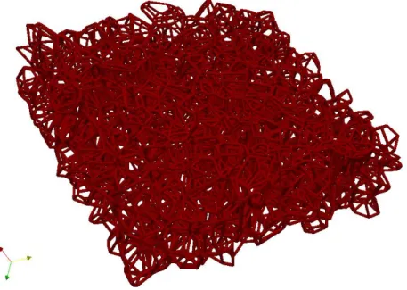
Fig. 6 Example of generated fiber image generated using the method described in Gostick (2013). The Voronoi lines (fibers) create polyhedral cages that define pore bodies.
The model used in this section has a random 3D architecture based on Delaunay tessellations to represent the pore space and Voronoi tessellations to represent the fiber structure. This model is illustrated in Fig.6 (see also Fig.5) and the procedure for generating it is described in details in Gostick (2013). This procedure is therefore not described again here. This type of network is referred to as a Voronoi network in the following.
Similarly as for the cubic network, Nz is the number of pores (a pore corresponds to a polyhedral cage in Fig.6) in the through plane direction whereas Nx is the number of cages (pores) in the in-plane directions (Ny = Nx).