July 21, 2017
Shape and spin determination of Barbarian asteroids
M. Devogèle
1, 2, P. Tanga
2, P. Bendjoya
2, J.P. Rivet
2, J. Surdej
1, J. Hanuš
2, 3, L. Abe
2, P. Antonini
4, R.A. Artola
5, M.
Audejean
4, 7, R. Behrend
4, 8, F. Berski
9, J.G. Bosch
4, M. Bronikowska
6, A. Carbognani
12, F. Char
10, M.-J. Kim
11, Y.-J.
Choi
11, C.A. Colazo
5, J. Coloma
4, D. Coward
13, R. Durkee
14, O. Erece
15, 16, E. Forne
4, P. Hickson
17, R. Hirsch
9, J.
Horbowicz
9, K. Kami´nski
9, P. Kankiewicz
18, M. Kaplan
15, T. Kwiatkowski
9, I. Konstanciak
9, A. Kruszewki
9, V.
Kudak
19, 20, F. Manzini
4, 21, H.-K. Moon
11, A. Marciniak
9, M. Murawiecka
22, J. Nadolny
23, 24, W. Ogłoza
25, J.L
Ortiz
26, D. Oszkiewicz
9, H. Pallares
4, N. Peixinho
10, 27, R. Poncy
4, F. Reyes
28, J.A. de los Reyes
29, T. Santana–Ros
9,
K. Sobkowiak
9, S. Pastor
29, F. Pilcher
30, M.C. Quiñones
5, P. Trela
9, and D. Vernet
2 (Affiliations can be found after the references)Received . . . ; accepted . . . ABSTRACT
Context.The so-called Barbarian asteroids share peculiar, but common polarimetric properties, probably related to both their shape and composition. They are named after (234) Barbara, the first on which such properties were identified. As has been suggested, large scale topographic features could play a role in the polarimetric response, if the shapes of Barbarians are particularly irregular and present a variety of scattering/incidence angles. This idea is supported by the shape of (234) Barbara, that appears to be deeply excavated by wide concave areas revealed by photometry and stellar occultations.
Aims.With these motivations, we started an observation campaign to characterise the shape and rotation properties of Small Main-Belt Asteroid Spectroscopic Survey (SMASS) type L and Ld asteroids. As many of them show long rotation periods, we activated a worldwide network of observers to obtain a dense temporal coverage.
Methods.We used light-curve inversion technique in order to determine the sidereal rotation periods of 15 asteroids and the con-vergence to a stable shape and pole coordinates for 8 of them. By using available data from occultations, we are able to scale some shapes to an absolute size. We also study the rotation periods of our sample looking for confirmation of the suspected abundance of asteroids with long rotation periods.
Results.Our results show that the shape models of our sample do not seem to have peculiar properties with respect to asteroids with similar size, while an excess of slow rotators is most probably confirmed.
Conclusions.
Key words. asteroids – asteroid shape – asteroid rotation
1. Introduction
Shape modeling is of primary importance in the study of aster-oid properties. In the last decades, ⇠ 1000 asteraster-oids have had a shape model determined by using inversion techniques1; most of
them are represented by convex shape models. This is due to the fact that the most used technique when inverting the observed light-curves of an asteroid – the so-called light-curve inversion – is proven to mathematically converge to a unique solution only if the convex hypothesis is enforced (Kaasalainen and Torppa 2001; Kaasalainen et al. 2001). At the typical phase angles ob-served for Main Belt asteroids, the light-curve is almost insen-sitive to the presence of concavities according to ˇDurech and Kaasalainen (2003). Although the classical light-curve inver-sion process cannot model concavities, Kaasalainen et al. (2001) point out that the convex shape model obtained by the inversion is actually very close to the convex hull of the asteroid shape. Since the convex hull corresponds to the minimal envelope that contains the non-convex shape, the location of concavities cor-responds to flat areas. Devogèle et al. (2015) developed the flat
1 See the Database of Asteroid Models from Inversion Techniques
(DAMIT) data base for an up-to-date list of asteroid shape models: http://astro.troja.m↵.cuni.cz/projects/asteroids3D/
surfaces derivation technique (FSDT) which considers flat sur-faces on such models to obtain indications about the possible presence of large concavities.
Cellino et al. (2006) reported the discovery of the anomalous polarimetric behaviour of (234) Barbara. Polarisation measure-ments are commonly used to investigate asteroid surface proper-ties and albedos. Usually, the polarisation rate is defined as the di↵erence of the photometric intensity in the directions paral-lel and perpendicular to the scattering plane (normalised to their sum): Pr = II??+IIkk. It is well known that the intensity of polarisa-tion is related to the phase angle, that is, to the angle between the light-source direction and the observer, as seen from the ob-ject. The morphology of the phase-polarisation curve has some general properties that are mainly dependent on the albedo of the surface. A feature common to all asteroids is a “negative polari-sation branch” for small phase angles, corresponding to a higher polarisation parallel to the scattering plane. For most asteroids, the transition to positive polarisation occurs at an “inversion an-gle” of ⇠ 20 . In the case of (234) Barbara, the negative polarisa-tion branch is much stronger and exhibits an uncommonly large value for the inversion angle of approximately 30 . Other Bar-barians were found later on (Gil-Hutton et al. 2008; Masiero and Cellino 2009; Cellino et al. 2014; Gil-Hutton et al. 2014;
Bag-nulo et al. 2015; Devogèle et al. 2017), and very recently, it was discovered that the family of Watsonia is composed of Barbar-ians (Cellino et al. 2014).
Several hypotheses have been formulated in the past to ex-plain this anomaly. Strong backscattering and single-particle scattering on high-albedo inclusions were invoked. Near-infrared (NIR) spectra exhibit an absorption feature that has been related to the presence of spinel absorption from flu↵y-type Calcium-Aluminium rich Inclusions (CAIs) (Sunshine et al. 2007, 2008). The meteorite analogue of these asteroids would be similar to CO3/CV3 meteorites, but with a surprisingly high CAI abundance (⇠ 30%), never found in Earth samples. If this inter-pretation is confirmed, the Barbarians should have formed in an environment very rich in refractory materials, and would con-tain the most ancient mineral assemblages of the Solar System. This fact link, the explanation of the polarisation to the pres-ence of high-albedo CAIs, is the main motivation for the study of Barbarians, whose composition challenges our knowledge on meteorites and on the mechanisms of the formation of the early Solar System.
The compositional link is confirmed by the evidence that all Barbarians belong to the L and Ld classes of the Small Main-Belt Asteroid Spectroscopic Survey (SMASS) taxonomy (Bus and Binzel 2002), with a few exceptions of the K class. While not all of them have a near-infrared spectrum, all Barbarians are found to be L-type in the DeMeo et al. (2009) NIR-inclusive classification (Devogèle et al. 2017).
However, the variety of polarimetric and spectroscopic prop-erties among the known Barbarians, also suggests that composi-tion cannot be the only reason for the anomalous scattering prop-erties. In particular, Cellino et al. (2006) suggested the possible presence of large concavities on the asteroid surfaces, resulting in a variety of (large) scattering and incidence angles. This could have a non-negligible influence on the detected polarisation, but such a possibility has remained without an observational verifi-cation up to now.
Recent results concerning the prototype of the class, (234) Barbara, show the presence of large-scale concavities spanning a significant fraction of the object size. In particu-lar, interferometric measurements (Delbo et al. 2009) and well-sampled profiles of the asteroid obtained during two stellar oc-cultations indicate the presence of large-scale concave features (Tanga et al. 2015). Testing the shape of other Barbarians for the presence of concavities is one of the main goals of the present study, summarising the results of several years of observation. To achieve this goal, we mainly exploit photometry to determine the shape, to be analysed by the FSDT. We compare our results with the available occultation data (Dunham et al. 2016) in or-der to check the reliability of the inverted shape model, scale in size, and constrain the spin axis orientation. We also intro-duce a method capable of indicating if the number of available light-curves is sufficient to adequately constrain the shape model solution.
As we derive rotation periods in the process, we also test an-other evidence, rather weak up to now: the possibility that Bar-barians contain an abnormally large fraction of “slow” rotators, with respect to a population of similar size. This peculiarity – if confirmed – could suggest a peculiar past history of the rotation properties of the Barbarians.
The article is organised as follows. In Sect. 2, we describe the observation campaign and the obtained data. Sect. 3 presents the approach that was followed to derive the shape models. A new method for analysing the shape model of asteroids is presented and tested on well-known asteroids. In Sect. 4, the characteristics
of some individual asteroids are presented as well as a general discussion about the main results of the present work. The inci-dence of concavities and the distribution of the rotation periods and pole orientations of L-type asteroids are presented. Finally Sect. 5 contains the conclusions of this work.
2. The observation campaigns 2.1. Instruments and sites
Our photometric campaigns involve 15 di↵erent telescopes and sites distributed on a wide range in Earth longitudes in order to optimise the time coverage of slowly rotating asteroids, with minimum gaps. This is the only strategy to complete light-curves when the rotation periods are close to 1 day, or longer, for ground-based observers.
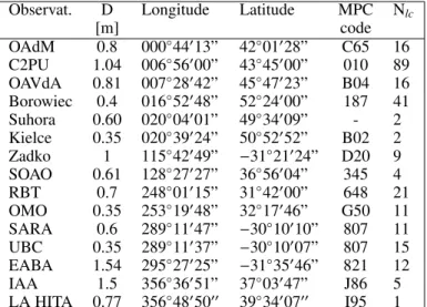
The participating observatories (Minor Planet Center (MPC) code in parentheses) and instruments, ordered according to their geographic longitudes (also Tab. 1), are:
– the 0.8m telescope of Observatori Astronòmic del Montsec (OAdM), Spain (C65),
– the 1.04m “Omicron” telescope at the Centre Pédagogique Planète et Univers (C2PU) facility, Calern observatory (Ob-servatoire de la Côte d’Azur), France (010),
– the 0.81m telescope from the Astronomical Observatory of the Autonomous Region of the Aosta Valley (OAVdA), Italy (B04),
– the 0.4m telescope of the Borowiec Observatory, Poland (187),
– the 0.6m telescope from the Mt. Suhora Observatory, Cra-cow, Poland,
– the 0.35m telescope from Jan Kochanowski University in Kielce, Poland (B02),
– the 1m Zadko telescope near Perth, Australia (D20), – the 0.61m telescope of the Sobaeksan Optical Astronomy
Observatory (SOAO), South Korea (345),
– the 0.7m telescope of Winer Observatory (RBT), Arizona, USA (648),
– the 0.35m telescope from the Organ Mesa Observaory (OMO), NM, USA (G50),
– the 0.6m telescope of the Southern Association for Re-search in Astrophysics (SARA), La Serena Observatory, Chile (807),
– the 0.35m telescope from the UBC Southern Observatory, La Serena Observatory, Chile (807),
– the 1.54m telescope of the Estaciòn Astrofìsica de Bosque Alegre (EABA), Argentina (821),
– the 1.5m telescope of the Instituto Astrofìsica de Andalucìa (IAA) in Sierra Nevada, Spain (J86),
– the 0.77m telescope from the Complejo Astronømico de La Hita, Spain (I95).
All observations were made in the standard V or R band as well as sometimes without any filter. The CCD images were re-duced following standard procedures for flat-field correction and dark/bias subtraction. Aperture photometry was performed by the experienced observers operating the telescopes, and the aux-iliary quantities needed to apply the photometric inversion (light-time delay correction, asterocentric coordinates of the Sun and the Earth) were computed for all the data.
The whole campaign is composed of 244 individual light-curves resulting from approximatively 1400 hours of observa-tion and 25000 individual photometric measurements of aster-oids. All the new data presented in this work are listed in Table A1 of Appendix A.
Observat. D Longitude Latitude MPC Nlc [m] code OAdM 0.8 000 44013” 42 01028” C65 16 C2PU 1.04 006 56000” 43 45000” 010 89 OAVdA 0.81 007 28042” 45 47023” B04 16 Borowiec 0.4 016 52048” 52 24000” 187 41 Suhora 0.60 020 04001” 49 34009” - 2 Kielce 0.35 020 39024” 50 52052” B02 2 Zadko 1 115 42049” 31 21024” D20 9 SOAO 0.61 128 27027” 36 56004” 345 4 RBT 0.7 248 01015” 31 42000” 648 21 OMO 0.35 253 19048” 32 17046” G50 11 SARA 0.6 289 11047” 30 10010” 807 11 UBC 0.35 289 11037” 30 10007” 807 15 EABA 1.54 295 27025” 31 35046” 821 12 IAA 1.5 356 36051” 37 03047” J86 5 LA HITA 0.77 356 4805000 39 3400700 I95 1 Table 1. List of the observatories participating in the observation cam-paigns, with telescope aperture (D), position, and number of light-curves. A rather good longitude coverage was ensured.
In addition to these observations, we exploited light-curves published in the literature. For the most ancient light-curves, the APC (Asteroid Photometric Catalogue (Lagerkvist et al. 2001)) was used. The most recent ones are publicly available in the DAMIT database ( ˇDurech et al. 2010).
As explained in the following section, we also used sparse photometry following the approach of Hanuš et al. (2011, 2013). The selected data sets come from observations from the United States Naval Observatory (USNO)-Flagsta↵ station (Interna-tional Astronomical Union (IAU) code 689), Catalina Sky Sur-vey Observatory (CSS, IAU code 703 (Larson et al. 2003)), and Lowell survey (Bowell et al. 2014).
The already published data used in this work are listed in Table B1 of Appendix B.
2.2. The target sample
We coordinated the observation of 15 asteroids, selected on the basis of the following criteria:
– Known Barbarians, with a measured polarimetric anomaly; – SMASS L or Ld type asteroids, exhibiting the 2 µm spinel
absorption band;
– members of dynamical families containing known Barbar-ians and/or L-type asteroids: Watsonia (Cellino et al. 2014), the dispersed Henan (Nesvorný et al. 2015); Tirela (Mothé-Diniz and Nesvorný 2008), renamed Klumpkea in Milani et al. (2014).
Fig. 1 shows the location (red dots) in semi-major axis and inclination of the asteroids studied in this work. In general, Bar-barians are distributed all over the main belt. The concentration in certain regions is a direct consequence of the identification of the Watsonia, Henan, and Tirela families. Future spectroscopic surveys including objects with a smaller diameter could better portray the global distribution.
For each of the 15 asteroids that have been targeted in this work, our observations have led to the determination of a new rotation period, or increase the accuracy of the previously known one. For eight of them, the light-curves dataset was sufficiently large to determine the orientation of the spin axis and a reliable convex shape model.
Table 2 lists the class in the Tholen (Tholen 1984), SMASS (Bus and Binzel 2002; Mothé-Diniz and Nesvorný 2008) and Bus-Demeo (DeMeo et al. 2009; Bus 2009) taxonomies of the 15 asteroids observed by our network. Each known Barbarian from polarimetry is labelled as “Y” in the corresponding column. The number of the family parent member is given in the correspond-ing column. The bottom part of Table 2 gives the same informa-tion for asteroids not observed by our network, but included in this work to increase the sample.
3. Modelling method and validation of the results 3.1. Shape modelling
The sidereal rotation period was searched for by the light-curve inversion code described in Kaasalainen and Torppa (2001) and Kaasalainen et al. (2001) over a wide range. The final period is the one that best fits the observations. It is considered as unique if the chi-square of all the other tested periods is > 10% higher. In order to obtain a more precise solution, sparse data are also included in the procedure, as described by Hanuš et al. (2013). When the determination of a unique rotation period is possible, the pole solution(s) can be obtained. As is well known, paired solutions with opposite pole longitudes (i.e. di↵ering by 180 ) can fit the data equally well. If four or less pole solutions (usually two sets of two mirror solutions) are found, the shape model is computed using the best fitting pole solution.
The accuracy of the sidereal rotation period is usually of the order of 0.1 to 0.01 times the temporal resolution interval P2/(2T) (where P is the rotation period and T is the length of
the total observation time span). For the typical amount of op-tical photometry we have for our targets the spin axis orienta-tion accuracy for the light-curve inversion method is, in general, ⇠ 5 / cos for and ⇠ 10 for (Hanuš et al. 2011).
All possible shapes were compared with the results derived from stellar occultations whenever they were available. The pro-jected shape model on the sky plane is computed at the occulta-tion epoch using the ˇDurech et al. (2011) approach. Its profile is then adjusted, using a Monte-Carlo-Markov-Chain algorithm, to the extremes of the occultation chords.
With this procedure, the best absolute scale of the model is found, thus allowing us to determine the size of the target. For ease of interpretation, the absolute dimensions of the ellipsoid best fitting- the scaled shape model and the volume-equivalent sphere Reqare computed.
In some cases, the result of stellar occultations also allows one to discriminate di↵erent spin axis solutions.
Eventually, the FSDT is used to analyse all the derived con-vex shape models. As this procedure depends on the presence of flat surfaces, we must ensure that the shape models are reliable. In fact, portions of the asteroid surface not sufficiently sampled by photometry, can also produce flat surfaces. We thus estab-lished the approach explained in the following section, allowing us to estimate the reliability of a shape derived by the light-curve inversion.
3.2. Shape validation by the bootstrap method
Our goal is to evaluate the reliability of shape model details, and to check if a set of light-curves provides a good determination of the spin parameters.
As mentioned above, the light-curve inversion process often provides several sets of spin parameters (rotation period and spin axis orientation) that fit the optical data equally well. In other
Semi-major axis (a) [AU]
2
2.5
3
3.5
Inclination (i) [°]
0
5
10
15
20
25
122 172 234 236 387 402 458 729 824 980 1332 1372 1702 2085 3844 15552 67255Fig. 1. Inclination versus semi-major axis plot of main-belt asteroids. The asteroids studied in this work are plotted as red circular dots, while the thinner blue dots represent the asteroid population as a whole.
cases, when only a few light-curves are available, the parameter set may converge with a single, but incorrect solution, often as-sociated with an incorrect rotation period. We see below that the bootstrapping method detects such cases.
Our approach consists in computing the shape model that best fits a subset of light-curves, randomly selected among all those that are available for a given asteroid. By studying how the fraction of flat surfaces ⌘sevolves with the number of selected
light-curves, we obtain a solid indication on the completeness of the data, that is, the need for new observations or not.
In more detail, we proceed as follows:
– First, a large number of light-curve samples is extracted from the whole data set. Each of these subsets may contain a num-ber of light-curves nlranging from nl =1 to all those avail-able (nl = Ndl). Sets of sparse data are also included in the
process and equal for all samples. In fact, the availability of a sparse data set is a necessary condition to apply the boot-strapping technique. Since shape models can sometimes be derived using sparse data only, they allow the inversion pro-cess to converge to a solution even for low values of nl.
– The second step consists in deriving the shape model cor-responding to all the light-curve samples generated in the previous step. The spin axis parameters found by using all the light-curves are exploited as initial conditions for each
inversion computation. If di↵erent sets of spin parameters are found with equal probability, the whole procedure is ex-ecuted for each of them.
– Once all the shape models are determined, we apply the FSDT in order to find the best value of ⌘s for each shape
model.
– The last step consists in determining the mean value and the dispersion of ⌘scorresponding to each subset group
charac-terised by nl=1, 2, 3, ..., Ndllight-curves.
An excess of flat surfaces is often interpreted as the qual-itative indication that the available photometry does not con-strain the shape model adequately. The addition of supplemen-tary light-curves is then a necessary condition to improve the shape. In our procedure, we make the hypothesis that, as the number of light-curves increases, the ⌘sparameter decreases. In
the process, the model converges to the convex hull of the real shape. Ideally, the only flat surfaces remaining should then cor-respond to concave (or really flat) topological features. Such a convergence should ideally show up as a monotonic decrease of ⌘stowards an asymptotic value for a large nl. Here, we apply our
procedure and show that our quantitative analysis is consistent with this assumption.
Asteroid Tholen SMASS DM Barbarian Family (122) Gerda ST L (172) Baucis S L Y (234) Barbara S Ld L Y (236) Honoria S L L Y (387) Aquitania S L L Y (402) Chloe S K L Y (458) Hercynia S L Y (729) Watsonia STGD L L Y 729 (824) Anastasia S L L (980) Anacostia SU L L Y (1332) Marconia Ld L (1372) Haremari L 729 (1702) Kalahari D L (2085) Henan L L 2085 (3844) Lujiaxi L L 2085 (15552) Sandashounkan 1400 (234) Barbara S Ld L Y (599) Luisa S K L Y (606) Brangane TSD K L 606 (642) Clara S L (673) Edda S S L (679) Pax I K L Y (1284) Latvia T L (2448) Sholokhov L L
Table 2. List of the targets observed by our network (upper part). Some targets that were not observed by us but discussed in this work were added in the lower part. The first column corresponds to the number and name of the considered asteroid. The columns Tholen (Tholen 1984), SMASS (Bus and Binzel 2002; Mothé-Diniz and Nesvorný 2008) and Bus-Demeo (DM) (DeMeo et al. 2009; Bus 2009) stand for the taxonomic class in these three types of taxonomy. The Barbarian column indicates whether or not the asteroid is considered as a Barbarian (Cellino et al. 2006; Gil-Hutton et al. 2008; Masiero and Cellino 2009; Bagnulo et al. 2015). Finally, the Family column indicates the number of the parent member of the family in which the asteroid is classified (606 for the Brangane, 729 for the Watsonia, 1400 for the Tirela/Klumpkea and 2085 for the Henan family).
We stress here that the number of possible subsets that can be extracted is potentially large, as it is given by the binomial coefficient⇣N
k
⌘ .
If the number of light-curves is below 14, all subsets are ex-ploited. If there are additional light-curves, the number of pos-sible combinations increases, but we do not generate more than 10, 000 random subsets to limit the computation time. Our re-sults show that this is not a limitation when the light-curve sam-ple is very rich.
3.2.1. Test on (433) Eros
The bootstrap method was first tested on (433) Eros for which the shape is well known thanks to the images taken by the NEAR mission (Gaskell 2008). A large number of dense photometric light-curves (N = 134) is also available for this asteroid which allows us to derive an accurate shape model using light-curve inversion.
The data set of (433) Eros contains 134 dense light-curves and 2 sets of sparse data. Fig. 2 shows the average of the flat surface fraction (⌘s) as a function of the number of dense
light-curves (Ndl) used for the shape modelling.
As expected (Fig. 2), the ⌘sversus Ndlcurve (hereafter called
the bootstrap curve) is monotonically decreasing. It is straight-forward to verify that an exponential function y = a exp ( bx)+c is well suited to fit the bootstrap curve. In this expression the c parameter corresponds to the asymptotic value ⌘a, that is, the ⌘s
Number of light curve
0 20 40 60 80 100 120 140
Mean fraction of flat surfaces
0.1 0.2 0.3 0.4 0.5 0.6 0.7 433 Eros f(x) = a exp( - b x) + c a = 0.49573 b = 0.017975 c = 0.13405 R = 0.99113 (lin)
Fig. 2. Bootstrap curves for the asteroid (433) Eros
that would be detected if a very large number of light-curves was used. In the case of (433) Eros we find ⌘a=0.134.
For a comparison to the “real” shape, we can take advantage of the detailed shape model of (433) Eros obtained by the analy-sis of the NEAR space probe images, obtained during the close encounter. For our goal, a low-resolution version (Gaskell 2008) is sufficient, and was used to check the result described above.
By taking the convex-hull (i.e. the smallest convex volume that encloses a non-convex shape), we obtain the shape model that, in an ideal case, the light-curve inversion should provide. In that specific case, the FSDT yields ⌘a = 0.12. This value is
within 6% of the value obtained by the bootstrapping method. This is a first indication that our approach provides a good ap-proximation and can be used to evaluate the “completeness” of a light-curve set.
We may compare our result to the value corresponding to the complete set of Ndl available light-curves. In this case,
⌘s = 0.18, a much larger discrepancy (20%) with respect to the
correct value. This result means that the convex shape model of (433) Eros (derived by photometry only) could probably be somewhat improved by adding new dense light-curves.
In the following sections, we apply this analysis to other ob-jects for the evaluation of their shape as derived from the photo-metric inversion.
3.2.2. Sensitivity of the bootstrap method to the spin axis coordinates
The behaviour of the bootstrap curve (exponentially decreasing) is related to the choice of the correct spin axis parameters.
This property is illustrated on the asteroid (2) Pallas. Even though Pallas has not been visited by a space probe, its spin axis orientation and shape are well known thanks to stellar occulta-tions and adaptive optics observaocculta-tions (Carry et al. 2010).
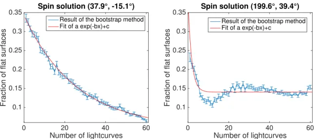
The other di↵erence with the case of (433) Eros is that there are less observed dense light-curves. As a matter of fact, the light-curve inversion provides two ambiguous solutions for the spin axis coordinates, at (37.9 , 15.1 ) and (199.6 , 39.4 ). Both poles yield the same RMS residuals for the fit to the light-curves. A priori, there is no way to know which solution is the best, without additional constraint such as disk-resolved obser-vations, since both solutions reproduce equally well the observed photometry. However, there is a clear di↵erence between the two when analysing the bootstrap curve (Fig. 3). The first solu-tion follows the well-defined exponential convergence providing ⌘a =0.045, which seems to be consistent with the shape model
as it is known so far. For the second spin axis orientation so-lution, we see that the bootstrap curve does not seem to follow the exponential trend. The corresponding ⌘a ⇠ 0.15 is in
contra-diction with the fact that the shape of (2) Pallas does not show any sign of large concave topological features. The rejection of the second pole solution is consistent with the result of stellar occultations and adaptive optics (Carry et al. 2010).
3.2.3. Distribution of flat surfaces across the available shape-model population.
The bootstrap method gives us information on the possible pres-ence of concave topological features. Here, a large number of as-teroid shape models are analysed. These shape models are used as a reference population with which the derived shape models of Barbarians can be compared.
This reference was constructed using the shape models avail-able on the DAMIT database ( ˇDurech et al. 2010). More than 200 asteroid shape models were analysed. For many of them, the re-sult of the bootstrap method clearly shows that more data would be needed to obtain a stable shape. In a minority of cases, we find a behaviour suggesting incorrect pole coordinates. We selected a sample of 130 shape models, for which the bootstrap curve had the expected, regular behaviour towards a convergence, and for them we computed ⌘a.
4. Results and interpretation
In Fig. 4, one example of a composite light-curve for two as-teroids observed by our network is shown. For each target, the synodic period (Psyn) associated to the composite light-curve is
provided. Additional light-curves are displayed in Appendix C. For the cases where too few light-curves have been obtained by our survey to derive a reliable synodic period, the sidereal pe-riod (Psid) determined based on multi-opposition observations
and obtained by the light-curve inversion method is used as an initial guess. In the case of (824) Anastasia, no error bars are provided since our observations were obtained during only one (very long) revolution. In Fig. 5 is displayed two examples of shape model derived in this work. Additional shape models are displayed in Appendix D. The bootstrap curves (see Sec. 3.2.1) are also shown for the di↵erent solutions of the pole orientation (except for (387) Aquitania for which no sparse data were used). Table 3 summarises the information about these asteroids, whose physical properties have been improved by our observations. Ta-ble 4 is the same as TaTa-ble 3, except that it lists asteroids that we did not directly observe ourselves, but that are relevant to our discussion.
4.1. Individual asteroids
In the following we compare our results for each asteroid to some data available in the literature; asteroid occultation results (Dunham et al. 2016) in particular.
In Figs. 6 to 9, the occultations data are represented in the so-called fundamental plane (i.e. the plane passing through the centre of the Earth and perpendicular to the observer-occulted star vector) ( ˇDurech et al. 2011). In that plane, the disappear-ance and reappeardisappear-ance of the occulted star are represented re-spectively by blue and red squares and the occultation chords represented by coloured continuous segments. Error bars on the disappearance and reappearance absolute timing are represented by discontinuous red lines. Negative observations (no occulta-tion observed) are represented by a continuous coloured line. Discontinuous segments represent observations for which no ab-solute timing is available. For each asteroid, the corresponding volume-equivalent radius is computed (corresponding to the ra-dius of a sphere having the same volume as the asteroid shape model). The dimensions of the ellipsoid best fitting the shape model are also given. The uncertainties on the absolute dimen-sions of the shape models adjusted to stellar occultations are de-rived by varying various parameters according to their own un-certainties. First, the di↵erent shape models obtained during the bootstrap method are used. The spin axis parameters are ran-domly chosen according to a normal distribution around their nominal values with standard deviation equal to the error bars given in Table 3. Finally the extremes of each occultation chord are randomly shifted according to their timing uncertainties. The observed dispersion in the result of the scaling of the shape model on the occultations chords is then taken as the formal un-certainty on those parameters.
The list of all the observers of asteroid occultations which are used in this work can be found in Appendix D (Dunham et al. 2016). In the following we discuss some individual cases.
(172) Baucis - There are two reported occultations. The first event is a single-chord, while the other (18 December 2015) has two positive chords and two negative ones, and was used to scale the shape model (Fig. 6). According to the fit of the shape model to the occultation chords, both pole solutions seemed equally likely. The two solutions give similar absolute
dimen-Number of lightcurves
0 20 40 60
Fraction of flat surfaces 0.1
0.15 0.2 0.25 0.3
0.35 Spin solution (37.9°, -15.1°) Result of the bootstrap method Fit of a exp(-bx)+c
Number of lightcurves
0 20 40 60
Fraction of flat surfaces 0.1
0.15 0.2 0.25 0.3
0.35 Spin solution (199.6°, 39.4°) Result of the bootstrap method Fit of a exp(-bx)+c
Fig. 3. Bootstrap curves for the asteroid (2) Pallas. The panels illustrate the curve obtained for di↵erent coordinates of the spin axis.
Rotational phase 0 0.5 1 1.5 Relative magnitude 2 2.05 2.1 2.15 2.2 2.25 2.3 2.35 Borowiec 131101 Borowiec 131202 Organ Mesa 140103 Organ Mesa 140110 Organ Mesa 140113 Organ Mesa 140127 Organ Mesa 140129 Borowiec 140205 C2PU 140207 Organ Mesa 140215 Organ Mesa 140219 C2PU 140217 Borowiec 140205 Kielce 140309 Borowiec 140313 Kielce 140320 Rotational phase 0 0.2 0.4 0.6 0.8 1 1.2 1.4 Relative magnitude 0 0.05 0.1 0.15 0.2 0.25 0.3 C2PU 040417 C2PU 130417 C2PU 130418 C2PU 130424 C2PU 130503 C2PU 130506 C2PU 130511 C2PU 130512 C2PU 130513 C2PU 130517 C2PU 130519 C2PU 130520 C2PU 130521 C2PU 130604 C2PU 130605 C2PU 130606
(236) Honoria, Psyn=12.3373 ± 0.0002 h (729) Watsonia, Psyn=25.19 ± 0.03 h
Fig. 4. Composite light-curves of two asteroids in our sample. Each light-curve is folded with respect to the synodic period of the object, indicated below the plot.
sions of (41.1 ± 2, 36.3 ± 1.8, 31.8 ± 1.6) and (40.8 ± 2.4, 36.1 ± 1.7, 33.5 ± 1.6) km, respectively. The corresponding volume-equivalent radii are Req=36.2±1.8 km and Req=36.7±1.8 km,
to be compared to the NEOWISE (Mainzer et al. 2016), AKARI (Usui et al. 2012) and IRAS (Tedesco 1989) radii: 35.3 ± 0.4, 33.5 ± 0.4 and 31.2 ± 0.6 km, respectively. Even though the oc-cultation observations cannot provide information about the best spin axis solution, the bootstrap curve indicates a clear prefer-ence for the one with retrograde rotation.
(236) Honoria - There are eight observed occultations. How-ever, over these eight events, only two have two positive chords (in 2008 with two positive chords and 2012 with three pos-itive chords). These were used to constrain the pole orienta-tion and scale the shape model. The result shows that the first pole solution ( 1 and 1 from Table 3) is the most plausible.
By simultaneously fitting the two occultations, the obtained di-mensions are (48.8 ± 1.4, 48.3 ± 1.3, 33.7 ± 1.0) km, and the volume-equivalent radius Req = 43.0 ± 2.1 km. In the case of
the second pole solution, the dimensions of the semi-axes are (52.3 ± 2.7, 52.1 ± 2.6, 37.1 ± 1.9) km and the equivalent radius is Req=45.6 ± 2.3 km. These solutions are compatible with the
NEOWISE, AKARI, and IRAS measurements which are respec-tively 38.9±0.6, 40.6±0.5 and 43.1±1.8 km. The fit of the shape model for the two pole solutions is shown in Fig. 7.
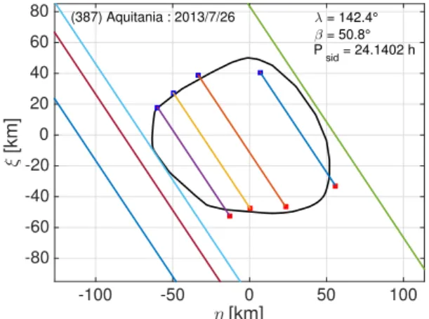
(387) Aquitania - For this asteroid, the result of the light-curve inversion process gives di↵erent solutions for the rotation period when sparse data are included. However, the noise on the sparse data is higher than the amplitude of the light-curves them-selves. For this reason we decided to discard them. As a conse-quence, we did not apply the bootstrap method to this asteroid.
There is one well sampled occultation of (387) Aquitania providing four positive and four negative chords. The adjust-ment of the unique solution of the shape model on the occul-tation chords shows a good agreement. The scaling leads to an equivalent radius Req=50.4 ± 2.5 km. The absolute dimensions
are (54.2 ± 2.7, 50.6 ± 2.5, 46.6 ± 2.3) km. This is consistent with the WISE (Masiero et al. 2011), AKARI, and IRAS radii, which are respectively 48.7 ± 1.7, 52.5 ± 0.7, and 50.3 ± 1.5 km. The fit of the shape model on the occultation chords is shown in Fig. 8. Hanuš et al. (2017) found a relatively similar model, spin axis solution (Psid = 24.14012 hours, = 123 ± 5 , and =
46 ± 5 ), and size (48.5 ± 2 km) using an independent approach. (402) Chloe - There are six reported occultations, but only two can be used to adjust the shape models on the occultation chords. These two occultations occurred on the 15 and 23 De-cember 2004. The result clearly shows that the first pole so-lution is the best one. The other one would require a defor-mation of the shape that would not be compatible with the constraints imposed by the negative chords. The derived
di-(172) Baucis, pole solution (14 , 57 ).
(236) Honoria, pole solution (196 , 54 ).
Fig. 5. Example of two asteroid shape models derived in this work. For both shape model, the reference system in which the shape is described by the inversion procedure, is also displayed. The z axis corresponds to the rotation axis. The y axis is oriented to correspond to the longest direction of the shape model on the plane perpendicular to z. Each shape is projected along three di↵erent viewing geometries to provide an overall view. The first one (left-most part of the figures) corresponds to a viewing geometry of 0 and 0 for the longitude and latitude respectively (the x axis is facing the observer). The second orientation corresponds to (120 , 30 ) and the third one to (240 , 30 ). The inset plot shows the result of the Bootstrap method. The x axis corresponds to the number of light-curves used and the y axis is ⌘a.
η [km] -50 0 50 ξ [km] -60 -40 -20 0 20 40 60 (172) Baucis : 2015/12/18 λ = 170.6° β = -63° P sid = 27.4097 h η [km] -60 -40 -20 0 20 40 60 ξ [km] -50 0 50 (172) Baucis : 2015/12/18 λ = 14.1° β = -57.2° P sid = 27.4096 h
Fig. 6. Fit of the derived shape models for (172) Baucis on the observed occultation chords from the 18 December 2015 event. The left panel represents the shape model corresponding to the first pole solution ( 1, 1). The right panel represents the shape model obtained using the second pole solution.
mensions of (402) Chloe, for the first spin axis solution, are (38.3±1.9, 33.7±1.7, 24.7±1.2) km and the equivalent radius is Req=31.3±1.6 km. The second spin solution leads to the
dimen-sions (46.9 ± 2.4, 41.3 ± 2.1, 29.0 ± 1.5) km and Req=38.3 ± 1.9 km. The NEOWISE radius is 27.7 ± 0.8 km while the AKARI and IRAS radii are 30.2 ± 1.5 and 27.1 ± 1.4 km, respectively, which agree with the first pole solution, but not with the
sec-ond one. The fit of the shape model on the occultation chords is shown in Fig. 9.
(824) Anastasia - The light-curve inversion technique pro-vided three possible pole solutions. However, two of them present a rotation axis which strongly deviates from the prin-cipal axis of inertia. This is probably related to the extreme elon-gation of the shape model. The light-curve inversion technique is
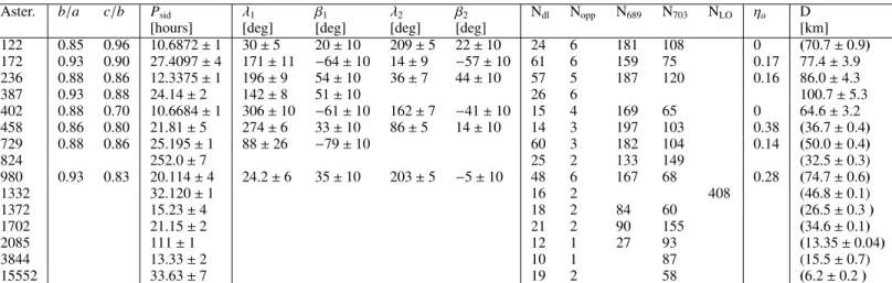
Aster. b/a c/b Psid 1 1 2 2 Ndl Nopp N689 N703 NLO ⌘a D
[hours] [deg] [deg] [deg] [deg] [km]
122 0.85 0.96 10.6872 ± 1 30 ± 5 20 ± 10 209 ± 5 22 ± 10 24 6 181 108 0 (70.7 ± 0.9) 172 0.93 0.90 27.4097 ± 4 171 ± 11 64 ± 10 14 ± 9 57 ± 10 61 6 159 75 0.17 77.4 ± 3.9 236 0.88 0.86 12.3375 ± 1 196 ± 9 54 ± 10 36 ± 7 44 ± 10 57 5 187 120 0.16 86.0 ± 4.3 387 0.93 0.88 24.14 ± 2 142 ± 8 51 ± 10 26 6 100.7 ± 5.3 402 0.88 0.70 10.6684 ± 1 306 ± 10 61 ± 10 162 ± 7 41 ± 10 15 4 169 65 0 64.6 ± 3.2 458 0.86 0.80 21.81 ± 5 274 ± 6 33 ± 10 86 ± 5 14 ± 10 14 3 197 103 0.38 (36.7 ± 0.4) 729 0.88 0.86 25.195 ± 1 88 ± 26 79 ± 10 60 3 182 104 0.14 (50.0 ± 0.4) 824 252.0 ± 7 25 2 133 149 (32.5 ± 0.3) 980 0.93 0.83 20.114 ± 4 24.2 ± 6 35 ± 10 203 ± 5 5 ± 10 48 6 167 68 0.28 (74.7 ± 0.6) 1332 32.120 ± 1 16 2 408 (46.8 ± 0.1) 1372 15.23 ± 4 18 2 84 60 (26.5 ± 0.3 ) 1702 21.15 ± 2 21 2 90 155 (34.6 ± 0.1) 2085 111 ± 1 12 1 27 93 (13.35 ± 0.04) 3844 13.33 ± 2 10 1 87 (15.5 ± 0.7) 15552 33.63 ± 7 19 2 58 (6.2 ± 0.2 )
Table 3. Summary of the results pertaining to our survey. The b/a and c/b columns represent the relative axis dimensions of the ellipsoid best fitting the shape model. The Psidcolumn indicates the sidereal rotation period of the asteroid in hours. The uncertainties are given with respect to the last digit. Columns nand n, with n = 1 and 2, represent the two or the unique pole solution(s). The Nxcolumns represent respectively the number of dense light-curves, the number of oppositions and the number of sparse points from the USNO (MPC code 689), Catalina (MPC code 703) and Lowell surveys. ⌘arepresents the fraction of flat surfaces present on the shape model as inferred by the bootstrap method. Finally, the D column represents the equivalent diameter of the sphere having the same volume as the asteroid shape model. When we were not able to scale the shape model of the asteroid, the NEOWISE diameter (Mainzer et al. 2016) (or WISE diameter (Masiero et al. 2011) when NEOWISE data are unavailable) is given in parentheses.
Asteroid b/a c/b Psid 1 1 2 2 ⌘a D Ref.
[hours] [deg] [deg] [deg] [deg] [km]
234 0.90 0.88 26.474 144 38 0.33 43.7 [1] 599 9.3240 71 [2] 606 0.82 0.92 12.2907 183 20 354 26 35.5 [3] 642 8.19 38.2 [4] 673 22.340 41.6 [5] 679 0.72 0.92 8.45602 220 32 42 5 0.38 51.4 [6] 1284 9.55 46 [7] 2448 10.061 43 [8]
Table 4. Same as Table 3, but for asteroids which were not observed during this campaign. The bootstrap method was not applied to (606) because the number of dense light-curves was not sufficient. References : [1] Tanga et al. (2015), [2] Debehogne et al. (1977), [3] Hanuš et al. (2011), [4] LeCrone et al. (2005), [5] Marciniak et al. (2016), [6] Marciniak et al. (2011), [7] Carreño-Carcerán et al. (2016), [8] Strabla et al. (2013)
known to have difficulty in constraining the relative length along the axis of rotation, in particular. In the case of highly elongated bodies, the principal axis of inertia is poorly constrained.
Two occultations were reported for this asteroid. The mod-els cannot fit the two occultations simultaneously using a single scale factor. We decided therefore not to present the shape model and spin solutions in this paper as new observations are required to better constrain the pole solution. Because of the very large rotation period of this asteroid, the presence of a possible tum-bling state should also be tested.
(2085) Henan - This asteroid possesses a relatively large ro-tation period. Based on our photometric observation, two syn-odic periods can be considered (110±1 hours and 94.3±1 hours). However, the light-curve inversion technique seems to support the first one based on our observations and sparse data.
4.2. Presence of concavities
We have applied the flat detection method (FSDT) described in Devogèle et al. (2015) to all the shape models presented in this paper, thus (Sec. 3.2) providing a quantitative estimate for the presence of concavities and for the departure of an asteroid shape from a smooth surface with only gentle changes of curvature.
Fig. 10 presents the result of the FSDT for the shape mod-els presented in this work (blue diamonds, see Tables 3 and 4). These results can be compared to the average value of ⌘a
com-puted by bins of 15 asteroids (red squares) using the asteroid population described in Sec. 3.2.3 (black dots).
From this distribution, a correlation between diameter and fraction of flat surfaces seems to be apparent. Such correlation is expected since small asteroids are more likely to possess ir-regular shapes than larger ones. However, the quality of aster-oid light-curves is directly correlated to the asteraster-oids diameter. For small asteroids (< 50 km), this e↵ect might also increase the mean value of ⌘a. Fig. 10 does not show clear di↵erences
between Barbarians and other asteroids, as Barbarians seem to populate the same interval of values. As expected, some aster-oids like Barbara show a large amount of flat surfaces, but this is not a general rule for Barbarians. Of course the statistics are still not so high, but our initial hypothesis that large concave topological features could be more abundant on objects having a peculiar polarisation does not appear to be valid in view of this first attempt of verification.
η [km] -50 0 50 ξ [km] -60 -40 -20 0 20 40 60 (236) Honoria : 2008/10/11 λ = 196° β = 54.2° P sid = 12.3376 h η [km] -50 0 50 ξ [km] -60 -40 -20 0 20 40 60 (236) Honoria : 2012/9/7 λ = 196°β = 54.2° P sid = 12.3376 h η [km] -50 0 50 ξ [km] -60 -40 -20 0 20 40 60 (236) Honoria : 2008/10/11 λ = 36.2° β = 44.5° P sid = 12.3376 h η [km] -50 0 50 100 ξ [km] -60 -40 -20 0 20 40 60 (236) Honoria : 2012/9/7 λ = 36.2° β = 44.5° P sid = 12.3376 h
Fig. 7. Fit of the derived shape models for (236) Honoria on the observed occultation chords from the 11 October 2011 and the 7 September 2012 events. The left panel represents the 2008 event with the top and bottom panels corresponding to the first and second pole solutions, respectively. The right panel is the same as the left one, but for the 2012 event.
η [km] -100 -50 0 50 100 ξ [km] -80 -60 -40 -20 0 20 40 60 80 (387) Aquitania : 2013/7/26 λ = 142.4° β = 50.8° P sid = 24.1402 h
Fig. 8. Fit of the derived shape model for (387) Aquitania on the ob-served occultation chords from the 26 July 2013 event.
4.3. Are Barbarian asteroids slow rotators ?
In this Section, we compare the rotation periods of Barbarians and Barbarian candidates with those of non-Barbarian type. At first sight the rotation period of confirmed Barbarian asteroids seems to indicate a tendency to have long rotation periods, as the number of objects exceeding 12h is rather large. For our analysis we use the sample of objects as in Tables 3 and 4. By considering
only asteroids with a diameter above 40 km, we are relatively sure that our sample of L-type asteroids is both almost com-plete, and not a↵ected by the Yarkovsky-O’Keefe-Radzievskii-Paddack e↵ect (Bottke et al. 2006). However, as only 13 aster-oids remain in the sample, we also consider a second cut at 30 km, increasing it to 18. As shown below, our findings do not change as a function of this choice.
We proceed by comparing the rotation period of the Barbar-ians with that of a population of asteroids that possess a similar size distribution. Since the distribution of rotation periods is de-pendent on the size of the asteroids, we select a sample of as-teroids with the same sizes, using the following procedure. For each Barbarian, one asteroid is picked out randomly in a popula-tion for which the rotapopula-tion period is known, and having a similar radiometric diameter within a ±5 km range. This way we con-struct a population of asteroids with the same size distribution as the Barbarians. We now have two distinct populations that we can compare. By repeating this process several times, we build a large number of populations of ‘regular’ asteroids. We can then check the probability that the distribution of rotation periods of such a reconstructed population matches the one of the Barbar-ians.
Considering the sample of asteroids with a diameter larger than 40 km, the sample is too small to derive reliable statistics. However, we notice that the median of the rotation period of the Barbarians is 20.1 hours while the median of the population regular asteroid is only 12.0 hours.
η [km] -40 -20 0 20 40 ξ [km] -20 -10 0 10 20 30 40 (402) Chloe : 2004/12/23 λ = 306.3° β = -61.1° P sid = 10.6684 h η [km] -50 0 50 ξ [km] -30 -20 -10 0 10 20 30 40 (402) Chloe : 2004/12/15 λ = 306.3° β = -61.1° P sid = 10.6684 h η [km] -50 0 50 ξ [km] -40 -20 0 20 40 60 (402) Chloe : 2004/12/15 λ = 163.5° β = -43.8° P sid = 10.6684 h η [km] -50 0 50 ξ [km] -40 -20 0 20 40 60 (402) Chloe : 2004/12/23 λ = 163.5° β = -43.8° P sid = 10.6684 h
Fig. 9. Fit of the derived shape models for (402) Chloe on the observed occultation chords from 15 and 23 December 2014 events. The leftmost part of the Figure represents the 15 event with the upper and lower parts corresponding to the first and second pole solutions, respectively. The rightmost part of the Figure is the same as the leftmost part, but for the 23 December event.
Diameter [Km]
Fraction of flat surfaces
0 0.1 0.2 0.3 0.4 0.5 0.6 0.7 0 50 100 150 200 250 540 Individual asteroids
Mean of individual asteroids Barbarians
Fig. 10. Values of ⌘aas a function of the asteroids diameters. The black dots correspond to individual asteroids. The red squares correspond to the mean values of ⌘aand diameter for bins of 15 asteroids. The blue diamonds correspond to Barbarian asteroids.
In order to improve the statistic, we can also take into ac-count asteroids with a diameter between 30 and 40 km. The median of the Barbarian asteroids is now 20.6 hours while the regular asteroids population has a median of 11.4 hours.
Fig. 11 represents the histograms of the rotation periods of Barbarian asteroids (with diameter > 30 km) compared to the population of regular asteroids constructed as described at the beginning of this section. The histogram of the Barbarian
aster-Fig. 11. Normalised histograms of the Barbarian compared to the his-togram asteroids having a diameter between 110 and 30 km.
oids shows a clear excess of long rotation periods and a lack of fast-spinning asteroids.
We adopt the two-samples Kolmogorov-Smirnov (KS) test to compare the distributions of Barbarians and regular asteroids.
This is a hypothesis test used to determine whether two pop-ulations follow the same distribution. The two-sample KS test returns the so-called asymptotic p-value. This value is an indi-cation of the probability that two samples come from the same population.
In our case, we found p = 0.6%, clearly hinting at two dis-tinct populations of rotation period.
In conclusion our results show that there is clear evidence that the rotations of Barbarian asteroids are distinct from those of the whole population of asteroids. The abnormal dispersion of the rotation periods observed for the Barbarian asteroids is more probably the result of a true di↵erence than a statistical bias.
5. Conclusions
We have presented new observations here for 15 Barbarian or candidate Barbarian asteroids. For some of these asteroids, the observations were secured by us during several oppositions. These observations allow us to improve the value of the rotation period. For eight of them, we were able to determine or improve the pole orientation and compute a shape model.
The shape models were analysed using a new approach based on the technique introduced by Devogèle et al. (2015). We show that this technique is capable of providing an indication about the completeness of a light-curve data set indicating whether or not further observations are required to better define a shape so-lution of the photometric inversion method. The extrapolation of the trend towards a large number of light-curves gives a more precise determination of ⌘s. This new method was applied to
a large variety of shape models in the DAMIT database. This allowed us to construct a reference to which the shape models determined in this work were compared. Our results show that there is no evidence that our targets have more concavities or are more irregular than a typical asteroid. This tends to infirm the hypothesis that large-scale concavities may be the cause of the unusual polarimetric response of the Barbarians.
The improvement and new determination of rotation peri-ods has increased the number of asteroids for which a reliable rotation period is known. This allows us to have an improved statistic over the distribution of rotation periods of the Barbarian asteroids. We show in this work possible evidence that the Bar-barian asteroids belong to a population of rotation periods that contains an excess of slow rotators, and lacks fast spinning as-teroids. The relation between the polarimetric response and the unusual distribution of rotation periods is still unknown.
Acknowledgements
The authors thank the referee for his comments, which improved the manuscript.
MD and JS acknowledge the support of the Université de Liège.
MD and PT acknowledge the support of the French “Pro-gramme Nationale de Planétologie".
Part of the photometric data in this work were obtained at the C2PU facility (Calern Observatory, O.C.A.).
NP acknowledges funding from the Portuguese FCT - Foun-dation for Science and Technology. CITEUC is funded by Na-tional Funds through FCT - Foundation for Science and Tech-nology (project: UID/ Multi/00611/2013) and FEDER - European Regional Development Fund through COMPETE 2020 -Operational Programme Competitiveness and Internationalisa-tion (project: POCI-01-0145-FEDER-006922).
SARA observations were obtained under the Chilean Tele-scope Allocation Committee program CNTAC 2015B-4.
PH acknowledges financial support from the Natural Sci-ences and Engineering Research Council of Canada, and thanks the sta↵ of Cerro Tololo Inter-American Observatory for techni-cal support.
The work of AM was supported by grant no. 2014/13/D/ST9/01818 from the National Science Centre, Poland.
The research of VK is supported by the APVV-15-0458 grant and the VVGS-2016-72608 internal grant of the Faculty of Sci-ence, P.J. Safarik University in Kosice.
MK and OE acknowledge TUBITAK National Observatory for a partial support in using T100 telescope with project number 14BT100-648.
References
Bagnulo, S., Cellino, A., Sterzik, M.F., 2015, MNRAS Lett., 446, L11 Barucci M., Fulchignoni M., Burchi R. and D’Ambrosio V., 1985, Icarus, 61,
152
Binzel R., 1987, Icarus, 72, 135
Bottke W.F., Vokrouhlick D., Rubincam D.P., Nesvorn D., 2006, Annual Review of Earth and Planetary Sciences, 34, 157
Bowell, E., Oszkiewicz, D. A., Wasserman, L. H., Muinonen, K., Penttilä, A., Trilling, D. E., 2014, Meteoritics & Planetary Science, 49, 95
Buchheim R., Roy R., Behrend R., 2007, The Minor Planet Bulletin, 34, 13 Bus S., Binzel R., 2002, Icarus, 158, 146
Bus, S. J., Ed., IRTF Near-IR Spectroscopy of Asteroids V1.0. EAR-A-I0046-4-IRTFSPEC-V1.0. NASA Planetary Data System, 2009.
Carreõ-Carcerán, A. et al., 2016, MPBu, 43, 92 Carry B. et al., 2010, Icarus, 205, 460
Cellino A., Belskaya I. N., Bendjoya Ph., di Martino M., Gil-Hutton R., Muinonen K. and Tedesco E. F., 2006,Icarus, 180, 565
Cellino A., Bagnulo S., Tanga P., Novakivoc B., Delbo M., 2014, MNRAS, 439, 75
Debehogne, H., Surdej, A., Surdej, J., 1977, A&A Suppl. Ser., 30, 375 DeMeo F., Binzel R., Slivan S and Bus S, 2009, Icarus, 160, 180
Denchev P., Shkodrovb V. and Ivanovab V., 2000, Planetary and Space Science, 48, 983
Delbo M., Ligori S., Matter A., Cellino A., Berthier J.,2009, The A.J., 694, 1228 Devogèle M., Rivet J. P., Tanga P., Bendjoya Ph., Surdej J., Bartczak P., Hanus
J., 2015, MNRAS, 453, 2232
Devogèle M. et al., 2017a, MNRAS, 465, 4335 Devogèle M. et al., 2017b, Submitted to Icarus
di Martino M, Blanco D., Riccioli D., de Sanctis G., 1994, Icarus, 107, 269 Dunham, D.W., Herald, D., Frappa, E., Hayamizu, T., Talbot, J., and Timerson,
B., Asteroid Occultations V14.0. EAR-A-3-RDR-OCCULTATIONS-V14.0. NASA Planetary Data System, 2016.
ˇDurech, J., Kaasalainen, 2003, M., A&A, 709, 404
ˇDurech, J., Sidorin, V., Kaasalainen, M., 2010, A&A, 513, A46 ˇDurech J. et al.,2010, Icarus, 214, 652
Gaskell, R.W., 2008, Gaskell Eros Shape Model V1.0. NEAR-A-MSI-5-EROSSHAPE-V1.0. NASA Planetary Data System
Gil-Hutton R., Cellino A., Bendjoya Ph., A&A, 2014, 569, A122
Gil-Hutton R., Mesa V., Cellino A., Bendjoya P., Peñaloza L., Lovos F., 2008, A&A, 482, 309
Gil-Hutton R., 1993, Revista Mexicana de Astronomia y Astrofisica, 25, 75 Hanuš J. et al, 2011, A&A, 530, A134
Hanuš J. et al, 2013, A&A, 551, 16 Hanuš J. et al, 2017, A&A, Accepted Harris A and Young J, 1989, Icarus, 81, 314
Harris A., Young J., Dockweiler T., Gibson J., Poutanen M., Bowell E., 1992, Icarus, 92, 115
Kaasalainen M., Torppa J., 2001, Icarus, 153, 24
Kaasalainen M., Torppa J., Muinonen K., 2001, Icarus, 153, 37
Lagerkvist, C.-I., Piironen, J., Erikson, A., 2001, Asteroid photometric cata-logue, fifth update (Uppsala Astronomical Observatory)
Larson, S., et al., 2003, BAAS, 35, AAS/Division for Planetary Sciences Meeting Abstracts #35, 982
LeCrone, C., Mills, G., Ditteon, R., 2005, MPBu, 32, 65
Mainzer et al., 2016, NEOWISE Diameters and Albedos V1.0. EAR-A-COMPIL-5-NEOWISEDIAM-V1.0. NASA Planetary Data System. Marciniak et al, 2011, A&A, 529, A107
Masiero J., Cellino A., 2009, Icarus, 199, 333 Masiero J. et al., ApJ, 2011, 741, 68
Mothé-Diniz T., Nesvorný, D., 2008, A&A 492, 593
Milani, A., Cellino A., Kneževi´c, Z., Novakovi´c, B., Spoto, F., Paolicchi, P., 2014, Icarus, 46, 239
Nesvorný, D., Broz, M., Carruba, V., 2015, Asteroids IV Oey J., 2012, MPB, 39, 145
Piclher F., 2009, The Minor Planet Bulletin, 36, 133 Schober H.J. , 1979, Astron. Astroph. Suppl., 8, 91
Sunshine et al., 2007, Lunar and Planetary Institute Science Conference Abstact, 1613
Sunshine et al., 2008, Science, 320, 514
Shevchenko V., Tungalag N., Chiorny V., Gaftonyuk N., Krugly Y., Harris A. and Young J., 2009, Icarus, 1514
Stephens R.D., 2013, MPB, 40, 34 Stephens R.D., 2013, MPB, 40, 178 Stephens R.D., 2014, MPB, 41, 226
Strabla, L., Quadri, U., Girelli, R., 2013, MPBu, 40, 232 Tanga P. et al., 2015, MNRAS, 448, 3382
Tedesco, E.F, 1989, in Asteroid II, 1090
Tholen, D.J. 1984, “Asteroid Taxonomy from Cluster Analysis of Photometry”. PhD thesis, University of Arizona.
Usui F. et al., 2012, The Astrophysical Journal, 762, 1 Warner B.D., 2009, MPB, 36, 109
Weidenschilling et al., 1990, Icarus, 86, 402
1 Université de Liège, Space sciences, Technologies and Astrophysics Research (STAR) Institute, Allée du 6 Août 19c, Sart Tilman, 4000 Liège, Belgium
e-mail: [email protected]
2 Université Côte d’Azur, Observatoire de la Côte d’Azur, CNRS,
Laboratoire Lagrange
3 Astronomical Institute, Faculty of Mathematics and Physics,
Charles University in Prague, Czech Republic
4 CdR & CdL Group: Light-curves of Minor Planets and Variable Stars, Switzerland
5 Estación Astrofísica Bosque Alegre, Observatorio Astronómico
Córdoba, Argentina
6 Institute of Geology, Adam Mickiewicz University, Krygowskiego 12, 61-606 Pozna´n
7 Observatoire de Chinon, Chinon, France 8 Geneva Observatory, Switzerland
9 Astronomical Observatory Institute, Faculty of Physics, A. Mick-iewicz University, Słoneczna 36, 60-286 Pozna´n, Poland
10 Unidad de Astronomía, Fac. de Ciencias Básicas, Universidad de Antofagasta, Avda. U. de Antofagasta 02800, Antofagasta, Chile 11 Korea Astronomy and Space Science Institute, 776 Daedeokdae-ro,
Yuseong-gu, Daejeon, Republic of Korea
12 Osservatorio Astronomico della regione autonoma Valle
d’Aosta,Italy
13 School of Physics, University of Western Australia, M013, Crawley WA 6009, Australia
14 Shed of Science Observatory, 5213 Washburn Ave. S,
Minneapo-lis,MN 55410, USA
15 Akdeniz University, Department of Space Sciences and Technolo-gies, Antalya, Turkey
16 TUBITAK National Observatory (TUG), 07058, Akdeniz
Univer-sity Campus, Antalya, Turkey
17 Department of Physics & Astronomy, University of British
Columbia, 6224 Agricultural Road, Vancouver, B.C. V6T 1Z1, Canada
18 Astrophysics Division, Institute of Physics, Jan Kochanowski Uni-versity, ´Swi etokrzyska 15,25-406 Kielce Poland
19 Laboratory of Space Researches, Uzhhorod National University, Daleka st., 2a, 88000, Uzhhorod, Ukraine
20 Institute of Physics, Faculty of Natural Sciences, University of P.J. Safarik, Park Angelinum 9, 040 01 Kosice, Slovakia
21 Stazione Astronomica di Sozzago, Italy
22 NaXys, Department of Mathematics, University of Namur, 8 Rem-part de la Vierge, 5000 Namur, Belgium
23 Instituto de Astrofísica de Canarias (IAC), E-38205 La Laguna, Tenerife, Spain
24 Departamento de Astrofísica, Universidad de La Laguna (ULL), E-38206 La Laguna, Tenerife, Spain
25 Mt. Suhora Observatory, Pedagogical University, Podchora¸˙zych 2, 30-084, Cracow, Poland
26 Instituto de Astrofísica de Andalucía, CSIC, Apt 3004, 18080
Granada, Spain
27 CITEUC – Centre for Earth and Space Science Research of the Uni-versity of Coimbra, Observatório Astronómico da Universidade de Coimbra, 3030-004 Coimbra, Portugal
28 Agrupación Astronómica Región de Murcia, Orihuela, Spain 29 Arroyo Observatory, Arroyo Hurtado, Murcia, Spain
30 4438 Organ Mesa Loop, Las Cruces, New Mexico 88011 USA
Appendix A: Summary of the new observations used in this work
Appendix B: Summary of previously published observations used in this work
Appendix C: Light-curves obtained for this work Appendix D: Shape models derived in this work Appendix E: List of observers for the occultation
Asteroid Date of observations Nlc Observers Observatory
(122) Gerda 2015 Jun 09 - Jul 06 6 M. Devogèle Calern observatory, France
(172) Baucis 2004 Nov 20 - 2005 Jan 29 2 F. Manzini Sozzago, Italy
2005 Feb 22 - Mar 1 3 P. Antonini Bédoin, France
2013 Mar 1 - Apr 25 10 A. Marciniak, M. Bronikowska Borowiec, Poland R. Hirsch, T. Santana,
F. Berski, J. Nadolny, K. Sobkowiak
2013 Mar 4 - Apr 17 3 Ph.Bendjoya, M. Devogèle Calern observatory, France
2013 Mar 5 - Apr 16 15 P. Hickson UBC Southern Observatory,
La Serena, Chile
2013 Mar 5 - 8 3 M. Todd and D. Coward Zadko Telescope, Australia
2013 Mar 29 1 F. Pilcher Organ Mesa Observatory, Las Cruces, NM
2014 Nov 13 1 M. Devogèle Calern observatory, France
2014 Nov 18 - 26 5 A. U. Tomatic, K. Kami´nski Winer Observatory (RBT), USA
(236) Honoria 2006 Apr 29 - May 3 3 R. Poncy Le Crès, France
2007 Jul 31 - Aug 2 3 J. Coloma, H. Pallares Sabadell, Barcelona, Spain
2007 Jun 21 - Aug 21 2 E. Forne, Osservatorio L’Ampolla, Tarragona, Spain 2012 Sep 19 - Dec 06 9 A. Carbognani, S. Caminiti OAVdA, Italy
2012 Aug 20 - Oct 28 6 M. Bronikowska, J. Nadolny Borowiec, Poland T. Santana, K. Sobkowiak
2013 Oct 23 - 2014 03 20 8 D. Oszkiewicz, R. Hirsch Borowiec, Poland A. Marciniak, P. Trela,
I. Konstanciak, J. Horbowicz
2014 Jan 03 - Feb 19 7 F. Pilcher Organ Mesa Observatory, Las Cruces, NM
2014 Feb 07 - Feb 17 2 M. Devogèle Calern observatory, France
2014 Mar 09 - 20 2 P. Kankiewicz Kielce, Poland
2015 Mar 21 - 22 2 W. Ogłoza, A. Marciniak, Mt. Suhora, Poland V. Kudak
2015 Mar 22 - Mai 07 3 F. Pilcher Organ Mesa Observatory, Las Cruces, NM (387) Aquitania 2012 Mar 22 - May 23 4 A. Marciniak, J. Nadolny, Borowiec, Poland
A. Kruszewski, T. Santana,
2013 Jun 26 - Jul 25 2 M. Devogèle Calern observatory, France
2014 Nov 19 - Dec 29 4 A. U. Tomatic, K. Kami´nski Winer Observatory (RBT), USA K. Kami´nski
2014 Nov 19 - Dec 18 2 M. Todd and D. Coward Zadko Telescope, Australia
2014 Dec 17 1 F. Char SARA, La Serena, Chile
2014 Dec 18 1 M. Devogèle Calern observatory, France
2015 Jan 10 - 11 2 Toni Santana-Ros, Rene Du↵ard IAA, Sierra Nevada Observatory 2015 Nov 27 - 2016 Feb 16 2 M. Devogèle Calern observatory, France
(402) Chloe 2015 Jul 01 - 14 2 M.C. Quiñones EABA, Argentina
(458) Hercynia 2013 May 20 - Jun 05 4 M. Devogèle Calern observatory, France 2014 Nov 27 - 28 2 M.-J. Kim, Y.-J. Choi SOAO, South Korea
2014 Nov 27 1 A. Marciniak Borowiec, Poland
2014 Nov 28 - 29 2 A.U. Tomatic, K. Kami´nski Winer Observatory (RBT), USA
2014 Nov 29 1 M. Devogèle Calern observatory, France
2014 Nov 30 1 N. Morales La Hita, Spain
(729) Watsonia 2013 Apr 04 - Jun 06 16 M. Devogèle Calern observatory, France 2014 May 26 - Jun 18 16 R. D. Stephens Santana Observatory
2015 Sep 25 1 O. Erece, M. Kaplan, TUBITAK, Turkey
M.-J. Kim
2015 Oct 05 1 M.-J. Kim, Y.-J. Choi SOAO, South Korea
2015 Oct 23 - Nov 30 5 M. Devogèle Calern observatory, France
(824) Anastasia 2015 Jul 05 - 25 7 M. Devogèle Calern observatory, France
Table A.1. New observations used for period and shape model determination which were presented in this work and observations that are not included in the UAPC.
Asteroid Date of observations Nlc Observers Observatory
(980) Anacostia 2005 Mar 15 - Mar 16 2 J.G. Bosch Collonges, France
2009 Feb 14 - Mar 21 6 M. Audejean Chinon, France
2012 Aug 18 - Nov 02 7 K. Sobkowiak, M. Bronikowska Borowiec M. Murawiecka, F. Berski
2013 Feb 22 - Feb 24 3 M. Devogèle Calern observatory, France
2013 Mar 27 - Apr 15 7 A. Carbognani OAVdA, Italy
2013 Dec 19 - Feb 23 11 A.U. Tomatic OAdM, Spain
2013 Dec 18 - Feb 07 2 R. Hirsch, P. Trela Borowiec, Poland
2014 Feb 22 - Mar 27 4 M. Devogèle Calern observatory, France 2014 Feb 25 - Mar 7 3 J. Horbowicz, A. Marciniak Borowiec, Poland
2014 Feb 27 1 A.U. Tomatic OAdM, Spain
2015 Mar 11 - May 28 5 F. Char SARA, La Serena, Chile
2015 Jun 09 1 M.C. Quiñones EABA, Argentina
(1332) Marconia 2015 Apr 12 - May 18 8 M. Devogèle Calern observatory, France 2015 May 20 1 A.U. Tomatic, K. Kami´nski Winer Observatory (RBT), USA
2015 Jun 03 1 R.A. Artola EABA, Argentina
(1372) Haremari 2009 Nov 03 - Dec 08 8 R. Durkee Shed of Science Observatory, Minneapolis, MN, USA 2014 Dec 11 - Feb 11 7 M. Devogèle Calern observatory, France
2015 Jan 10 - 11 2 T. Santana-Ros, R. Du↵ard IAA, Sierra Nevada Observatory, Spain (1702) Kalahari 2015 Apr 29 - May 18 3 M. Devogèle Calern observatory, France
2015 May 19 1 A. U. Tomatic, K. Kami´nski Winer Observatory (RBT), USA
2015 May 20 1 M.-J. Kim, Y.-J. Choi SOAO, South Korea
2015 Jun 04 - Jul 08 8 C.A. Alfredo EABA, Argentina
(2085) Henan 2015 Jan 09 - 10 2 A. U. Tomatic OAdM, Spain
2015 Jan 11 1 T. Santana-Ros, R. Du↵ard IAA, Sierra Nevada Observatory, Spain 2015 Jan 14 - 15 2 M. Todd and D. Coward Zadko Telescope, Australia
2015 Jan 14 - Feb 11 7 M. Devogèle Calern observatory, France
2015 Mar 11 1 F. Char SARA, La Serena, Chile
(3844) Lujiaxi 2014 Nov 12 - Dec 23 5 M. Devogèle Calern observatory, France 2014 Nov 20 - Dec 18 2 M. Todd and D. Coward Zadko Telescope, Australia 2014 Nov 20 1 A.U. Tomatic, K. Kami´nski Winer Observatory (RBT), USA
2014 Dec 25 - 26 2 A.U. Tomatic OAdM, Spain
(15552) 2014 Oct 29 - Nov 25 7 A. U. Tomatic, K. Kami´nski Winer Observatory (RBT), USA Sandashounkan 2014 Oct 30 - Nov 13 2 M. Devogèle Calern obervatory, France
2014 Nov 20 1 A. U. Tomatic OAdM, Spain
Asteroid Date of observations Nlc Reference
(122) Gerda 1987 Jul 28 - Aug 01 2 Shevchenko et al. (2009) 1981 Mar 13 - 25 3 di Martino et al. (1994) 1981 Mar 18 - 19 2 Gil-Hutton (1993) 2003 Mai 02 - 09 3 Shevchenko et al. (2009) 2005 Sep 11 - Oct 04 2 Shevchenko et al. (2009) 2005 Sep 31 - Nov 28 3 Buchheim et al. (2007) 2009 Apr 01 - 03 3 Pilcher (2009)
(172) Baucis 1984 May 11 1 Weidenschilling et al. (1990) 1989 Nov 21 1 Weidenschilling et al. (1990) (236) Honoria 1979 Jul 30 - Aug 22 7 Harris and Young (1989)
1980 Dec 30 - 1981 Feb 1 7 Harris and Young (1989) (387) Aquitania 1979 Aug 27 - 29 3 Schober et al. (1979)
1981 May 30 1 Barucci et al. (1985) 1981 May 30 - Jul 24 8 Harris et al. (1992) (402) Chloe 1997 Jan 19 - Mar 02 5 Denchev et al. (2000)
2009 Feb 07 - 17 4 Warner (2009) 2014 May 15 - 16 2 Stephens (2014)
(458) Hercynia 1987 Feb 18 1 Binzel (1987)
(729) Watsonia 2013 Jan 21 - Feb 14 8 Stephens (2013) (980) Anacostia 1980 Jul 20 - Aug 18 5 Harris and young (1989) (1332) Marconia 2012 Aug 27 - Sep 11 6 Stephens (2013) (1702) Kalahari 2011 Jul 28 - Aug 26 10 Oey (2012)
Rotational phase 0 0.2 0.4 0.6 0.8 1 Relative magnitude 3.1 3.12 3.14 3.16 3.18 3.2 3.22 3.24 3.26 3.28 C2PU 150609 C2PU 150624 C2PU 150625 C2PU 150630 C2PU 150705-06 Rotational phase 0 0.1 0.2 0.3 0.4 0.5 0.6 0.7 0.8 0.9 1 Relative magnitude 7.3 7.35 7.4 7.45 7.5 7.55 7.6 7.65 7.7 7.75 Sozzago 041120 Sozzago 050129 Bédoin 050222 Bédoin 050223 Bédoin 050301
(122) Gerda: 2015 opposition; Psyn=10.6872 ± 0.0001 h (172) Baucis: 2004-2005 opposition; Psyn=27.417 ± 0.005 h
Rotational phase 0 0.2 0.4 0.6 0.8 1 1.2 1.4 Relative magnitude 11.8 11.85 11.9 11.95 12 12.05 Borowiec 130103 Borowiec 130303 Borowiec 130403 Borowiec 130503 Hickson 130503 Hickson 130903 Hickson 131003 Hickson 131203 Borowiec 130313 Hickson 131403 Borowiec 131403 Hickson 131803 Hickson 131903 Hickson 132103 Hickson 132203 Borowiek 132903 Hickson 131504 Rotational phase 0 0.1 0.2 0.3 0.4 0.5 0.6 0.7 0.8 0.9 1 Relative magnitude 1.34 1.36 1.38 1.4 1.42 1.44 1.46 1.48 1.5 1.52 C2PU 141113 RBT 141118 RBT 141119 RBT 141121 RBT 141125 RBT 141126
(172) Baucis: 2013 opposition; Psyn=27.4096 ± 0.0004 h (172) Baucis: 2014 opposition; Psyn=27.42 ± 0.01 h
Rotational phase 0 0.1 0.2 0.3 0.4 0.5 0.6 0.7 0.8 0.9 1 Relative magnitude 12.92 12.93 12.94 12.95 12.96 12.97 12.98 12.99 Cres 060429 Cres 060430 Cres 060503
(236) Honoria: 2006 opposition; Psyn=12.35 ± 0.10 h
Rotational phase 0 0.1 0.2 0.3 0.4 0.5 0.6 0.7 0.8 0.9 1 Relative magnitude 11.16 11.18 11.2 11.22 11.24 11.26 11.28 11.3 11.32 11.34 Ampolla 070621 Sabadell 070731 Sabadell 070802 Ampolla 070821
(236) Honoria: 2007 opposition; Psyn=12.34 ± 0.02 h
Rotational phase 0 0.2 0.4 0.6 0.8 1 1.2 1.4 Relative magnitude -3.15 -3.1 -3.05 -3 -2.95 -2.9 Borowiec 120819 Borowiec 120823 Borowiec 120829 OAVdA 120919 OAVdA 120920 OAVdA 120921 Borowiec 120923 OAVdA 121003 OAVdA 121010 OAVdA 121012 Borowiec 121018 Borowiec 121028 OAVdA 121116 OAVdA 121206
(236) Honoria: 2012 opposition; Psyn=12.337 ± 0.001 h
Rotational phase 0 0.1 0.2 0.3 0.4 0.5 0.6 0.7 0.8 0.9 1 Relative magnitude 0.25 0.3 0.35 0.4 Borowiec 150321 Borowiec 150322 Organ Mesa 150322 Organ Mesa 150326 Organ Mesa 150507
(236) Honoria: 2015 opposition; Psyn=12.33 ± 0.01 h Fig. C.1. Composite light-curves of asteroids studied in this works.
Rotational phase 0 0.1 0.2 0.3 0.4 0.5 0.6 0.7 0.8 0.9 1 Relative magnitude 0.85 0.9 0.95 1 1.05 Borowiec 120322 Borowiec 120423 Borowiec 120425 Borowiec 120523
(387) Aquitania: 2012 opposition; Psyn=24.15 ± 0.02 h
Rotational phase 0 0.1 0.2 0.3 0.4 0.5 0.6 0.7 0.8 0.9 1 Relative magnitude -0.34 -0.33 -0.32 -0.31 -0.3 -0.29 -0.28 -0.27 -0.26 C2PU 130626 C2PU 130725
(387) Aquitania: 2013 opposition; Psyn=24.15 ± 0.15 h
Rotational phase 0 0.1 0.2 0.3 0.4 0.5 0.6 0.7 0.8 0.9 1 Relative magnitude 1.1 1.15 1.2 1.25 1.3 1.35 ZADKO 141101 RBT 141119 SARA 141217 C2PU 141218 RBT 141227 RBT 141228 RBT 141229 IAA 150110 IAA 150111 Rotational phase 0 0.1 0.2 0.3 0.4 0.5 0.6 0.7 0.8 0.9 1 Relative magnitude 3.54 3.56 3.58 3.6 3.62 3.64 3.66 3.68 C2PU 151127 C2PU 160225
(387) Aquitania: 2014-2015 opposition; Psyn=24.14 ± 0.02 h (387) Aquitania: 2015-2016 opposition; Psyn=24.147 h
Rotational phase 0 0.1 0.2 0.3 0.4 0.5 0.6 0.7 0.8 0.9 1 Relative magnitude -0.1 -0.05 0 0.05 0.1 0.15 EABA 150701 EABA 150714 Rotational phase 0 0.1 0.2 0.3 0.4 0.5 0.6 0.7 0.8 0.9 1 Relative magnitude 3.94 3.96 3.98 4 4.02 4.04 4.06 C2PU 130520 C2PU 130521 C2PU 130604 C2PU 130605
(402) Chloe: 2015 opposition; Psyn=10.70 ± 0.05 h (458) Hercynia: 2013 opposition; Psyn=21.8 ± 0.1 h
Rotational phase 0 0.1 0.2 0.3 0.4 0.5 0.6 0.7 0.8 0.9 1 Relative magnitude -0.2 -0.1 0 0.1 0.2 0.3 0.4 0.5 SOAO 141027 Borowiec 141027 RBT 141028 SOAO 141028 C2PU 141029 RBT 141029 La Hita 141030 RBT 141030 Rotational phase 0 0.2 0.4 0.6 0.8 1 1.2 Relative magnitude 1.8 1.85 1.9 1.95 2 2.05 TUBITAK 150925 SOAO 151005 C2PU 151023 C2PU 151101 C2PU 151125 C2PU 151127 C2PU 151130
(458) Hercynia: 2014 opposition; Psyn=21.81 ± 0.03 h (729) Watsonia: 2015 opposition; Psyn=25.190 ± 0.003 h Fig. C.1. Continued