Cluster expansion method for evolving weighted networks having vector-like nodes

Proceedings of the 3rd Polish Symposium on Econo- and Sociophysics, WrocÃlaw 2007

Cluster Expansion Method

for Evolving Weighted Networks

Having Vector-Like Nodes

M. Ausloos

_{and M. Gligor}

a_{GRAPES, SUPRATECS, U.Lg}

B5a Sart-Tilman, B-4000 Li`ege, Belgium

b_{National College Roman Voda Roman-5550, Neamt, Romania}

The cluster variation method known in statistical mechanics and con-densed matter is revived for weighted bipartite networks. The decomposition (or expansion) of a Hamiltonian through a finite number of components, whence serving to define variable clusters, is recalled. As an illustration the network built from data representing correlations between (4) macro-economic features, i.e. the so-called vector components, of 15 EU countries, as (function) nodes, is discussed. We show that statistical physics princi-ples, like the maximum entropy criterion points to clusters, here in a (4) variable phase space: Gross Domestic Product, Final Consumption Expen-diture, Gross Capital Formation and Net Exports. It is observed that the

maximum entropy corresponds to a cluster which does not explicitly include

the Gross Domestic Product but only the other (3) “axes”, i.e. consumption, investment and trade components. On the other hand, the minimal entropy clustering scheme is obtained from a coupling necessarily including Gross Domestic Product and Final Consumption Expenditure. The results con-firm intuitive economic theory and practice expectations at least as regards geographical connexions. The technique can of course be applied to many other cases in the physics of socio-economy networks.

PACS numbers: 89.75.Fb, 89.65.Gh, 89.75.Hc, 87.23.Ge

1. Introduction

In physics one is often interested about models with a finite number N of degrees of freedom, hereby denoted by s = (s1, s2, . . . , sN), taking sometimes

dis-crete values, in contrast to continuous ones, as in field theories. For instance, the variables si could take values [0 or 1] (binary variables), [–1,+1] (Ising spins), or

[1, 2, . . . q] (Potts variables). Network nodes and/or links can possess such degrees of freedom which indicate the role of a few variables for characterizing or tying

nodes together; these variables serve, e.g., to be exemplifying clusters, commu-nities, . . . in the network. Several network characterization techniques based on related discrete value algebra exist in the literature [1, 2].

Let us recall that statistical mechanical models are defined through an energy function, like a Hamiltonian, H = H(s); the corresponding probability distribution at thermal equilibrium is the Boltzmann distribution

p(s) = 1

Zexp(−H(s)), (1)

where the inverse temperature β = (kBT )−1 has been absorbed into the

Hamilto-nian as often conventionally done; Z = exp(−F) =X

s

exp(−H(s)) (2)

is called the partition function and F the free energy. The Hamiltonian is typically a sum of terms, each involving a small number of variables.

A technique which has been of interest a long time ago in condensed matter is the cluster variation approximation method [3–5]. The free energy or the Hamil-tonian is expanded through a series in the variables by a systematic projection in order to define the interaction energy at each successive cluster size level. We re-introduce the technique here, suggesting its power for discussing network prop-erties. The technique appears to be very general and could be useful to sort out features not observed otherwise. Whence for better framing the concept and reju-venating the vocabulary we re-outline some theoretical consideration and rewrite well known formulae.

We take as an example and for illustration a finite size network, one made of nodes being EU countries characterized by their most usual (macroeconomic) features. The fluctuation correlations between these serve to define the so-called adjacency matrix, whence the weights of the links of the network. Some “discussion section” will indicate the interest of projecting the Hamiltonian, in an appropriate phase space in order to observe features. One property being measured will be the system entropy which is clearly a mapping of p(s) into macroscopic-like features based on economic indicators.

2. Theoretical considerations

A useful representation of interacting units (spins, agents, fields,. . . ) is given by the factor graph. A factor graph [6] is a bipartite graph made of variable nodes i, j, . . ., one for each variable, and function nodes a, b, . . ., one for each interaction term of the Hamiltonian. A link joins a variable node i and a function node a if and only if i ∈ a, that is the variable siappears in Ha, the term of the Hamiltonian

associated to a. The Hamiltonian can then be written as H =

N

X

a

Ha(sa) (3)

Hamiltonian into terms describing clusters of different (increasing) sizes and func-tionalities has been shown to be of great interest, see [7], e.g. when one applies renormalization group-like techniques.

In combinatorial optimization problems, the Hamiltonian plays the role of a cost function and one is often interested in the low temperature limit T → 0, where only minimal energy states (ground states) have a nonvanishing probability. Probabilistic graphical models are usually defined in a slightly different way [8]. For example, in the case of Markov random fields, also called Markov networks, the joint distribution over all variables is given by

p(s) = 1 b Z Y a ψa(sa), (4)

where ψa is called the potential, and

b Z =X s Y a ψa(sa). (5)

Of course, a statistical mechanical model described by the Hamiltonian (3), corresponds to a probabilistic graphical model with potentials ψa = exp(−Ha),

and corresponding Z = bZ and F = bF.

Next we define a cluster α as a subset of the factor graph such that if a func-tion node belongs to α, then all the variable nodes sαalso belong to α; we notice

that the converse needs not be true, otherwise the only legitimate clusters would be the connected components of the factor graph. Given a cluster we can write its probability distribution, defined as the ratio between the number of realized connections and the number of all possible connections, as

pα(sα) =

X

s∈α

p(s) (6)

and its entropy Sα(sα) = −

X

s∈α

p(s) ln p(s). (7)

3. Illustration

As a short illustration, let us consider the function nodes to be countries and the variables to be macroeconomic indicators [9], i.e.:

1. Consider the nodes to be the first (in time) 15 EU countries. Let the country names be abbreviated according to the Roots Web Surname List (RSL) [10] which uses 3 letters standardized abbreviations.

2. Suppose that we are interested in a vector describing each country (Hamil-tonian or) “thermodynamic state” with 4 components, i.e. s1 ≡ Gross

Do-mestic Product (GDP), s2 ≡ Final Consumption Expenditure (FCE), s3≡

Gross Capital Formation (GCF), and s4≡ Net Exports (NEX). The World

Bank database [11] is here used as data source. Let the data be taken from 1994 to 2004 for GDP and from 1994 to 2003 for FCE, GCF and NEX, respectively.

The yearly fluctuations of these four variables are easily calculated and their auto- and cross-correlation matrices easily obtained; see e.g. a discussion for GDP in [12, 13] and more detail elsewhere [14]. Essentially, the correlations can be calculated for a time window of given size moving along the time axis; these are used for getting the statistical distances among countries, e.g. A and B, for various time window sizes T at various times t, where t is the final point of the interval, i.e. ds(A, B)(t,T )= q 2[1 − C(t,T )(A, B)] (8) as in [15] where C(t,T )(A, B) =

hABi(t,T )− hAi(t,T )hBi(t,T )

q (hA2_i

(t,T )− hAi2_{(t,T )})(hB2i(t,T )− hBi2_{(t,T )})

. (9)

The brackets h. . .i denote the expectation value of the “A, B time series”, here in the interval (t − T, t).

These distances are thus mapped onto ultrametrical distances, as in the classical minimum spaning tree (MST) method. By calculating the statistical dis-tances with respect to the average value of the index (seen here as for an “average” country), we get a country hierarchy that proves to be changing from a time inter-val to another when the (constant size) time window is moved over the full time span. The correlation coefficients refer to the movement of the countries inside this hierarchy.

In order to exemplify this method, the corresponding steps for s2 ≡ FCE

are explicitly shown below (for s1 ≡ GDP the first steps are explicitly described

in [16]). After the (virtual) “average” country is introduced in the system, the statistical distances corresponding to the fixed 5 years moving time win-dow can be calculated and set in increasing order. The minimal path length (MPL) connections to the “average” country can be established for each coun-try in every time interval (Table I). The resulting hierarchy is readily found to be changing from a time interval to another. The above procedure is repeated for each macroeconomic indicator, leading to similar three Tables to Table I. Next, a time independent “correlation matrix” can be built, at this stage for the country movement fluctuations inside the hierarchy, i.e. averaging the relative TABLE I The MPL distances to the “average country”. Indicator: FCE (≡ s2). The moving

time window size is T = 5 years for the data [11] taken from 1994 to 2003.

aut bel deu dnk esp fin fra gbr grc irl ita lux nld prt swe 94–98 0.88 0.65 0.85 0.88 0.65 0.37 0.65 0.65 0.65 0.65 0.37 0.65 0.65 0.65 0.65 95–99 0.79 0.79 0.79 0.81 0.79 0.41 0.79 0.79 0.93 0.79 0.53 0.59 0.79 0.79 0.79 96–00 1.02 1.02 1.02 1.02 1.02 1.02 1.02 1.02 1.02 1.02 0.26 1.02 1.02 1.02 1.02 97–01 0.51 0.51 0.51 0.65 0.51 0.73 0.88 0.51 0.65 0.51 0.33 0.88 0.51 0.51 0.51 98–02 0.52 0.52 0.52 0.96 0.52 0.66 0.95 0.65 0.96 0.52 0.35 1.19 0.52 0.52 0.52 99–03 0.45 0.42 0.45 1.00 0.45 0.53 0.40 0.46 1.00 0.42 0.30 0.92 0.45 0.45 0.45

TABLE II The correlation matrix of EU-15 country movements inside the hierarchy. Indicator: FCE. The moving time window size is 5 years for data taken from 1994 to 2003.

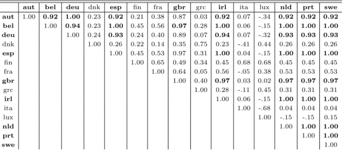
aut bel deu dnk esp fin fra gbr grc irl ita lux nld prt swe aut 1.00 0.92 1.00 0.23 0.92 0.21 0.38 0.87 0.03 0.92 0.07 -.34 0.92 0.92 0.92 bel 1.00 0.94 0.23 1.00 0.45 0.56 0.97 0.28 1.00 0.06 -.15 1.00 1.00 1.00 deu 1.00 0.24 0.93 0.24 0.40 0.89 0.07 0.94 0.07 -.32 0.93 0.93 0.93 dnk 1.00 0.26 0.22 0.14 0.35 0.75 0.23 -.41 0.44 0.26 0.26 0.26 esp 1.00 0.45 0.53 0.97 0.31 1.00 0.04 -.15 1.00 1.00 1.00 fin 1.00 0.65 0.49 0.34 0.45 0.68 0.68 0.45 0.45 0.45 fra 1.00 0.64 0.05 0.56 -.05 0.38 0.53 0.53 0.53 gbr 1.00 0.40 0.97 0.03 0.02 0.97 0.97 0.97 grc 1.00 0.28 -.11 0.45 0.31 0.31 0.31 irl 1.00 0.06 -.15 1.00 1.00 1.00 ita 1.00 -.68 0.04 0.04 0.04 lux 1.00 -.15 -.15 0.15 nld 1.00 1.00 1.00 prt 1.00 1.00 swe 1.00

MPL fluctuations between countries. In so doing, the moving-average-minimal--path- length (MAMPL) method leads us to a set of M = 4 correlation matrices (one for each index), having the size N × N , where N = 15 is the number of countries under consideration here. For example, Table II, for FCE (≡ s2). Nota bene the matrix is symmetric (half of the elements are shown) but not all elements are necessarily positive.

Let us suppose that we filter these (four) second correlation matrices in order to retain a few terms, those which lead us to build a network for which the weights (i.e. the correlation coefficients) are greater than e.g. 0.9. The correlation coefficients, e.g. in the case of the variable node s2(FCE fluctuations), as given in

Table II, are emphasized in bold for those ≥ 0.9 at each couple of function nodes. Due to the filtering, one can easily see that not all 15 countries have at least one “bold node”, i.e. are connected through the variable node s2 (FCE), but only

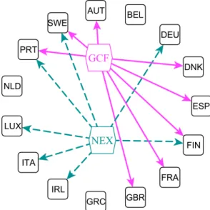
nine of them, namely AUT, BEL, DEU, ESP, GBR, IRL, NLD, PRT, and SWE. In Fig. 1, these nine countries are connected through the variable node FCE (the dashed arrows).

The above procedure can be repeated for GDP, GCF, and NEX, whence ob-taining the other “clusters” in Figs. 1 and 2, with respectively 9, 8 and 7 countries (for this filter value). Let us notice that GRC does not belong to any cluster∗_.

The cluster contributions to the Hamiltonian can thus be the variable s2.

Then one obtains that the cost function H associated to the factor graph (Figs. 1, 2) based on these four variables reads

∗_{GRC does not appear in the Hamiltonian, because (see Figs. 1, 2) GRC is not}

connected to the other countries through any siby a link having a weight greater than

0.9. If the linkage threshold is established to a lower value, e.g.|C| ≥ 0.8, its function node appears as (GRC)(s1, s4), i.e. it belongs to the same clusters as Italy.

Fig. 1. The factor graph associated to the first 15 EU country connections, according to the strongest correlations in the GDP and FCE.

Fig. 2. The factor graph associated to the first 15 EU country connections, according to the strongest correlations in the GCF and NEX.

H = H1+ H2+ H3+ H4,

where

H1= (LUX)(s4) + (NLD)(s2),

H3= (ESP)(s2, s3) + (FIN)(s3, s4) + (FRA)(s1, s3) + (DEU)(s1, s2, s4)

+(GBR)(s1, s2, s3) + (IRL)(s1, s2, s4), H4= (PRT)(s1, s2, s3, s4) + (SWE)(s1, s2, s3, s4),

from which one could write the equilibrium probability distribution, the partition function and the free energy, introduced here above.

4. Discussion

Instead of writing a Hamiltonian as a function of the function nodes, let us project the dynamics of the factor graph into a phase space spanned by the variable nodes. Let us recall that a cluster α was defined as a subset of the factor graph such that if a function node belongs to α, then all the variable nodes sα

also belong to α. We can write all the possible combinations of the four variable nodes and find the Hamiltonian corresponding to function nodes. Let us take for example the combination (s1≡ GDP; s2≡ FCE; s3≡ GCF). Then, the function

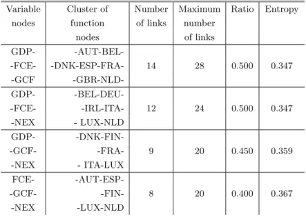
nodes connected only to these three variables (not necessarily to all of them) and TABLE III

Clustering of the first 15 EU countries in a 4-variable factor graph approach after filtering (see text) and projecting in a 3-variable node phase space; the number of links in the cluster, the maximum possible number of links, subsequently the relevant ratio, and the entropy of each cluster are given.

Variable Cluster of Number Maximum Ratio Entropy nodes function of links number

nodes of links GDP- -AUT-BEL--FCE- -DNK-ESP-FRA- 14 28 0.500 0.347 -GCF -GBR-NLD-GDP- -BEL-DEU--FCE- -IRL-ITA- 12 24 0.500 0.347 -NEX - LUX-NLD GDP- -DNK-FIN--GCF- -FRA- 9 20 0.450 0.359 -NEX - ITA-LUX FCE- -AUT-ESP--GCF- -FIN- 8 20 0.400 0.367 -NEX -LUX-NLD

not to the fourth one (s4 ≡ NEX) are AUT, BEL, DNK, ESP, FRA, GBR, and

NLD. This means a cluster that we can see in the first row in Table III. The same can be done for the other three combinations, leading to another set of clusters.

In so doing clustering [17] properties appear through e.g. an entropy, Eq. (7). The values are given in Table III for the clusters made of three variable nodes. As a not obvious consequence of this cluster analysis technique, it is observed that the maximum entropy (0.367) corresponds to the clustering which does not explicitly include the GDP but only the consumption, investment, and trade components. Another point can be deduced from the minimal entropy (0.347) clustering scheme, i.e. it is obtained from the coupling between GDP and FCE. The results confirm intuitive economic theory and practice expectations at least as regards geographi-cal connexions. However, deep discussions of these findings are left for economists. In conclusion, let us recall the frame of our work and our findings: relevant microscopic description of a system relies on a coarse-grained reduction of its internal variables. We have presented a way to do so for a bipartite graph having on one hand countries, on the other hand macroeconomy indicators. We have obtained a Hamiltonian description. The technique can of course be generalized and applied to many other socioeconomy networks.

5. Conclusion

Complex networks have become an active field of research in physics [18]. These systems are usually composed of a large number of internal components (the nodes and links), and describe a wide variety of systems of high intellectual and technological importance. Relevant questions pertain to the characterization of the networks. Investigations of the case of directed and/or weighted networks are not so common. The occurrence of community clustering for networks having nodes possessing a vector-like characteristics has been rarely studied. We have attempted to do so through a revival of some clustering variation method in the framework of some macroeconomy study.

We have taken as an example the weighted fully connected network of the N = 15 first countries forming the European Union in 2005 (EU-25). The ties be-tween countries are supposed to result (be proportional) to the degree of similitude of the macroeconomic fluctuations annual rates of four macroeconomic indicators, i.e. GDP, FCE, GCF, and NEX over ca. a 15 year time span.

Averaging the yearly increment correlations a weighted bipartite network has been built having the four “degrees of freedom” and the fifteen “countries” on the other hand as basis. The analysis shows the importance of N -body interac-tions in particular when observing the macroeconomy states as a function of time. This leads to identify and display clusters of countries, clusters resulting from projections onto a high-dimensional phase space spanned by indicators, taken as independent variables. This approach generalizes usual projection methods by ac-counting for the complex geometrical connections resulting from vector-like nodes.

In particular such a measure of collective habits does fit the usual and practi-cal expectations defined by politicians, journalists, or economists, through so-practi-called “common factors” [19, 20]. The analysis reveals geographical connexions indeed. It is expected that the technique can be applied to many types of physical and socioeconomic networks.

Acknowledgments

M.G. would like to thank the Francqui Foundation for financial support thereby having facilitated his stay in Li`ege. This work was part of investiga-tions stimulated and supported by the European Commission through the Critical Events in Evolving Networks (CREEN) Project (FP6-2003-NEST-Path-012864). M.A. thanks the FENS 07 organizers for their invitation and as usual very warm welcome in WrocÃlaw.

References

[1] R. Albert, A.-L. Barabasi, Rev. Mod. Phys. 74, 47 (2002).

[2] S.N. Dorogovtsev, J.F.F. Mendes, Evolution of Networks: From Biological Nets

to the Internet and WWW, Oxford Univ. Press, Oxford 2003.

[3] R. Kikuchi, Phys. Rev. 81, 988 (1951).

[4] M. Kurata, R. Kikuchi, T. Watari, J. Chem. Phys. 21, 434 (1953). [5] R. Kikuchi, S.G. Brush, J. Chem. Phys. 47, 195 (1967).

[6] A. Pelizzola, J. Phys. A 38, R309 (2005).

[7] G. Biroli, O. Parcollet, G. Kotliar, Phys. Rev. B 69, 205108 (2004). [8] P. Smyth, Pattern Recogn. Lett. 18, 1261 (1997).

[9] S.N. Durlauf, D.T. Quah, in: Handbook of Macroeconomics, Eds. J.B. Taylor, M. Woodford, North-Holland Elsevier Sci., Dordrecht 1999, p. 231.

[10] http://helpdesk.rootsweb.com/codes/.

[11] http://devdata.worldbank.org/query/default.htm.

[12] J. Miskiewicz, M. Ausloos, Int. J. Mod. Phys. C 17, 317 (2006). [13] M. Ausloos, R. Lambiotte, Physica A 382, 16 (2007).

[14] M. Gligor, M. Ausloos, J. Econ. Integration 23, 297 (2008). [15] R.N. Mantegna, Eur. Phys. J. B 11, 193 (1999).

[16] M. Gligor, M. Ausloos, Eur. Phys. J. B 57, 139 (2007). [17] D.J. Watts, S.H. Strogatz, Nature 393, 440 (1998).

[18] R. Pastor-Satorras, A. Vespignani, Evolution and Structure of the Internet:

A Statistical Physics Approach, Cambridge University Press, Cambridge 2004;

R. Pastor-Satorras, M. Rubi, A. Diaz-Guilera, Statistical Mechanics of Complex

Networks, Lect. Notes Phys., Vol. 625, Springer, Berlin 2003.

[19] T. Mora, Appl. Econ. Lett. 12, 937 (2005). [20] S. Barrios, E. Strobl, Econ. Lett. 82, 71 (2004).