Sound Field Modeling in Architectural Acoustics using a Diffusion
Equation Based Model
Nicolas Fortin1,2, Judicaël Picaut*2, Alexis Billon3, Vincent Valeau4 and Anas Sakout1
1University of La Rochelle, 2LCPC, 3University of Liège, 4Université de Poitiers-ENSMA-CNRS *Corresponding author: Laboratoire Central des Ponts et Chaussées, Route de Bouaye, BP 4129,
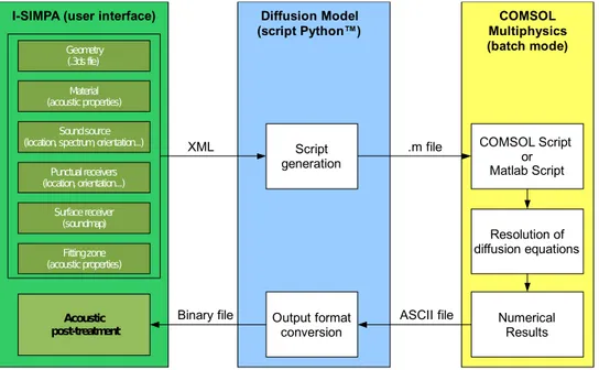
Abstract: In this paper, an implementation of a model for room-acoustic predictions in COMSOL Multiphysics is presented. The model (called diffusion model) is based on the solving of diffusion equations instead of classical wave equations and allows simulating the sound propagation in complex geometries at high frequency. Instead of using COMSOL Multiplysics to solve directly the problem, a specific tool has been developed. It is composed of a user-friendly interface (I-Simpa) which manipulates all the physical data of the problem (geometries, acoustic properties and elements…) and generates an interoperability script to execute COMSOL Multiplysics via the generation of .m file scripts. Then, numerical results are processed by I-Simpa for the acoustic post-treatment and results display, like sound levels, reverberation times…
Keywords: Room-acoustic, diffusion equation model, script file generation.
1. Introduction
The modeling of sound-fields in rooms has attracted considerable attention in recent decades. For “real rooms”, i.e., with complex shapes, partially diffusely reflecting surfaces, coupled spaces, fitted zones, computer methods such as the ray-tracing model have been developed and are now very popular. However, by increasing the complexity of the room shape, the computation time increases dramatically and can take several hours for engineering accuracy.
In recent years, an alternative approach to predict the diffuse sound field in arbitrary rooms has been proposed mainly by the authors1-7 and
others contributors8-10. This model, based on a
physical analogy with the diffusion of particles in a scattering medium, was derived to predict the spatial variations of the reverberant sound field in rooms, for both steady-state and time-varying sources. The model has been applied with success to empty homogeneous rooms, long enclosures, industrial halls with fitted zones, coupled spaces, and allows the modeling of acoustic transmission through walls, mixed diffuse-specular reflection at walls, as well as atmospheric absorption.
In order to solve the diffusion equations of the model, authors have initially used the FEMLAB package together with MATLAB®.
More recently, the authors have upgraded the diffusion model to use COMSOL Multiphysics, in an equivalent manner as already presented by Jing and Xiang.11-12 However, at this time, the
analogy between the acoustical problem (material, sound sources, receivers, fitting zones…) and the diffusion problem (see Section 2) has to be carried out manually in COMSOL Multiphysics. In an operational point of view, an acoustician in a design office should be able to use the diffusion model without knowledge of COMSOL Multiphysics, like classical acoustic software. So, the development of a specific user interface that manages all input acoustic data and runs COMSOL Multiphysics in background (see section 3) is necessary.
2. Acoustic diffusion model 2.1 Diffusion equation
The present study uses a model initially derived by Ollendorff and further developed by the authors1 for modeling the acoustics of
enclosed spaces with diffusely reflecting surfaces. The model is based on an analogy between the sound diffusion in a room and the diffusion of particles in a medium containing spherical scattering obstacles.
This analogy requires only that the mean free path is equivalent for both diffusion media. In room acoustics, a common analytical expression for the mean free path in a room with diffusely reflecting boundaries is = 4V/S, where V and S are the volume and the surface of the room. Then, given the slow rates of change with time involved in diffusion phenomena, the local particle-density flux J(r,t) can be approximated as the gradient of the particle density,
) , ( ) , (r t Dgradw r t J . (1)
Under this assumption, the particle density can be shown to be the solution of a diffusion equation. The analogy with room acoustics allows the assumption that the acoustic energy density in the room w(r,t) at a position r and time t is governed by the diffusion equation,
0 ) , ( ) , ( w t t w D t r r , (2)
where is the Laplace operator and D is the so-called diffusion constant, defined as
3
c
2.2 Absorption at walls
The last diffusion equation (3) expresses the diffuse propagation within the enclosure without considering absorption by the boundaries S. The energy exchanges at a diffusely reflecting surface can be described using the following form:1 ) , ( ) , ( ) , ( t D w t hw r t n r n r J , (4)
where h is the so-called exchange coefficient. Under this condition, the local energy flux at boundaries is assumed to be proportional to the local energy density. Several expressions have been proposed to model this absorption phenomenon, such as: 4
4
c
h , (5)
for low absorption ( being the Sabine’s absorption coefficient), 4 ) 1 ln( c h , (6)
for higher absorption (Eyring absorption). However, the last expression presents a singularity for =1 (total absorption). A modified boundary condition has then been proposed by Jing and Xiang, as:9
) 2 ( 2 c h . (7)
2.3 Transmission through walls
The complete phenomenon of the reverberant sound field transmission between rooms connected through partition walls can be considered in order to predict the acoustic energy distribution in networks of rooms, for both diffuse and non diffuse configurations 6.
Let us consider for example the case of two rooms coupled through a coupling area (part of the partition wall). The first room (the source room, i.e. containing the sound source) of volume V1 and surface area S1 (without the
coupling area) is separated from the second room (the adjacent room) of volume V2 and surface
area S2 (without the coupling area) by a partition
wall. The coupling area that permits sound transmission is defined by its surface S12 and its
absorption coefficient 12. By considering
internal losses in the partition wall through the dissipation coefficient , 12 can be written as a
function of the transmission loss R (or the transmission coefficient =10−R/10) such as
12 = + .
Then, a diffusion equation similar to equation (2) must be considered for each room (i.e. each one with its own density energy, w1 and w2 in this example). Moreover the boundary
equation (4) must be modified as:
2 1 12 4 1 1 1 w c w h w D n , (8)
on the source room side, and
1 2 21 2 4 2 2 h w cw w D n , (9)
on the adjacent room side, where h12is
the exchange coefficient of the wall partition.
2.4 Boundary conditions: mixed diffuse-specular wall reflection
Mixed diffuse and specular reflections are defined by the diffusion coefficient s (ratio between diffuse and total energy reflected at the room surface). To simulate this phenomenon, the diffusion constant D can be modified as follows:7
D K m
D , (10)
where K is an empirical correction, verifying the empirical relation: 1.549 ln(s) 2.238 K . (11) 2.5 Atmospheric absorption
In the diffusion equation (2), the atmospheric attenuation is not taken into account, although this phenomenon can be significant at high frequencies, particularly for large enclosures. Following the same approach as the one for deriving the diffusion equation (2), the atmospheric attenuation term can be introduced in the model, leading to a modified expression of the diffusion constant, noted now D’:5
m D D 1 ' (12)
where m is the coefficient of atmospheric attenuation (in m-1). However, the sound
absorption being usually very small over a mean free path, one can consider thereafter that D’D.
Similarly, by introducing the atmospheric attenuation term in the derivation of the diffusion model, the diffusion equation for the energy density in the room becomes
0 w mcw w D t . (13) 2.6 Fitting zones
The diffusion model can also be modified for estimating the sound field in fitted rooms, i.e. containing many obstacles (machines, stockpiles, benches etc., i.e. the “fittings”), such as industrial workrooms, classrooms, offices etc. These obstacles scatter and absorb sound, so that the acoustic behavior of the fitted room is different from an empty room.
The modified diffusion model combines then two diffusion approaches (one for the diffusion by objects and one for the diffusion by room surfaces) into a single diffusion process.
In the following, the variables referring to the scattering objects, or fittings, will be denoted by the subscript f, and the variables referring to the room will be denoted by the subscript r. Moreover, let us consider that the scatterers are modeled statistically by their density nf, their
average scattering cross-section Qf and their
absorption coefficient αf. For a propagation
medium containing only scattering obstacles – i.e. in a free field with obstacles – the mean free path for a particle between two collisions is λf =
1/Qfnf. For an empty room, the mean free path
for a particle between two collisions is λr =
1/Qrnr = 4V/S λ, as expressed before. Lastly,
one can show that the diffusion equation (2) can
be modified in order to take the fitting into account as: 3 0 f w f c w w t D t , (14)
with the modified diffusion constant
r D f D r D f D t D , (15)
where Dr D is the classical diffusion constant.
3. User interface I-Simpa 3.1Principle
On a practical point of view (i.e. for COMSOL Multiphysics users), the numerical definition of the problem could be carried out from the “Stationary analysis” or the “Time-dependent analysis” in the “Coefficient form” option of the “PDE Modes” located in the “Applications Modes” of the “Model Navigator”, and then by setting the corresponding parameters (D, h, m) in the “Subdomain Settings” and the “Boundary Settings” windows, for each subdomain and boundary.
For coupled rooms, the numerical system of diffusion equations (one diffusion equation for each coupled room), with the associated boundary conditions for each side, must be solved numerically as coupled equations. An iterative solving of this set of equations is then required.
However, as presented in the introduction and depicted in figure 1, a specific interface (called I-Simpa) with associated Python™ scripts have been developed in order that all calculations with COMSOL Multiphysics are realized in batch mode, using .m script files generated by I-Simpa. Then all data are manipulated through exchange-files and interpreted by I-Simpa.
3.2 I-Simpa functionalities
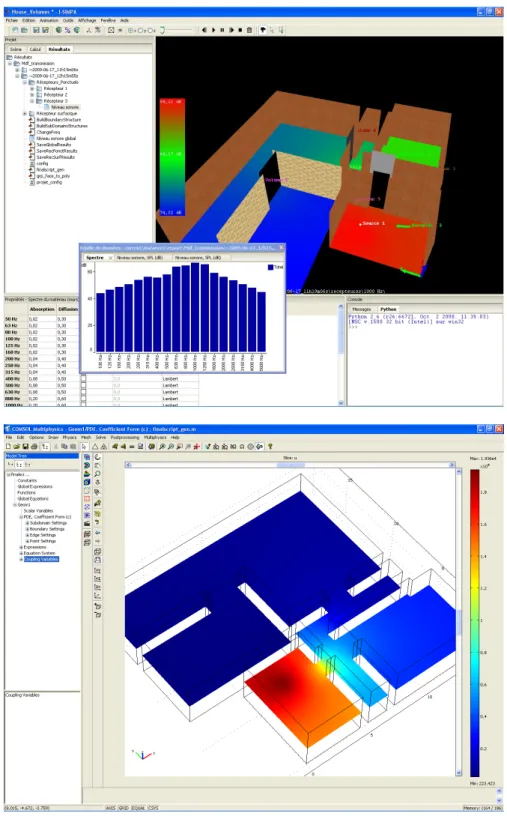
I-Simpa is a GUI developed by the authors (1) to run several models of sound propagation (particularly the diffusion model), (2) to import and to manipulate geometries (3ds format), (3) to manage all acoustics data (like sound sources, acoustic receivers, materials, fitting zones and others properties, which are needed for the chosen sound propagation calculation..), and lastly (4) to carry out the post-processing of numerical results in order to obtain the main usual acoustical parameters (sound pressure level, room acoustics parameters, sound decay curves, energy flow…). An example application of I-Simpa (a network of acoustically coupled rooms) is given in figure 2, with its equivalent COMSOL Multiphysics vizualisation.
3.3 Script generation (.m file)
When choosing the diffusion model in the I-Simpa interface, a Python™ script is used to generate the .m file script that can be “understood” by COMSOL Multiphysics and run in batch mode (with the comsolbatch.exe executable file). The following steps are considered (the script example that is given below represents a simple cubic room with one sound source. Note also that some lines are broken (symbol […]) in order to limit the number of lines in the example):
1. Header generation;
% COMSOL Multiphysics Model M-file % Generated by I-Simpa, $Date: 2009/09/19 16:09:48 $)
2. Definition of constants (speed of sound; reference pressure; volume, surface, mean free path and diffusion coefficient for each room; source size…)
fem.const = {'cel','343.2', ... 'Vol','60.0000009537', ... 'S','94.0', ... 'lamb','4*Vol/S', ... 'Dif','lamb*cel/3', ... 'r_source','0.2', ... 'V_source','4/3*pi*r_source^3', ... 'Pref','2e-05', ... 'rho','1.2' ... }; disp('Building model');
3. Vertices definition of the room geometry in a
Nx3 array, noted verts (N vertices with 3
coordinates x, y and z). The .3ds file if converted in a geometry (vertices and faces) usable in COMSOL Multiphysics;
verts=[5.000000,-0.000000,-0.000000; […];];
4. Faces definition of the room geometry: for example in an array facearr from verts; facearr={ grp_face_to_poly(verts,[1,2,3;1,3,4]) […]}; Geometry (.3ds file) Material (acoustic properties) Sound source (location, spectrum, orientation...)
Punctual receivers (location, orientation...) Surface receiver (soundmap) Fitting zone (acoustic properties) COMSOL Script or Matlab Script Numerical Results Script generation Output format conversion Resolution of diffusion equations
I-SIMPA (user interface) COMSOL
Multiphysics (batch mode) Diffusion Model (script Python™) XML Acoustic post-treatment Binary file .m file ASCII file
5. Subdomains definition: each room, fitted zone, acoustic sources are defined separately in a structure array s. In the diffusion model, sound sources are represented by spheres with a given energy density;
s1=sphere3('r_source','pos', {'2.000000','2.000000','2.000000'},'ax is', {'0','0','1'},'rot','0','const',fem.co nst); dom0=geomcoerce('solid',facearr([1, 2, 3, 4, 5, 6])); disp('Model builded.'); clear s s.objs={s1,dom0}; s.name={'Domaine de s1','Domaine de dom0'}; s.tags={'s1','dom0'};
6. Definition of the list of materials in a structure array mat.materials (PDE coefficients q, h and g, and type of boundary conditions (Neumann or Dirichlet) for each face). Note that material properties depend on the frequency band);
mat.materials.q={{0,0,0,0,0,0,0,0,0,0, 0,0,0,0,0,0,0,0,0,0,0,0,0,0,0,0,0}, {'cel*0.0400/4','cel*0.0400/4',[…]}}; mat.materials.name={…
'Materiau sources','mat id:101',… 'mat id:100','mat id:0'};
mat.materials.h={1,0,0,0}; mat.materials.type={'neu','dir',… 'dir','dir'}; mat.materials.g={0,0,0,0}; mat.assoc={[1,1,1,1,1,1,1,1], … [2, 3, 3, 3, 3, 3]}; mat.faces={[],[1, 2, 3, 4, 5, 6]}; 7. Equation definition for each subdomain:
(PDE coefficients f, a, da and c); vol.names= {'Domaine de s1',… 'Domaine de dom0'}; vol.f=… {{'(10^(65.68/10))/V_source', […]}; vol.a=… {0,{'0.000018*cel',[…]}}; vol.da= {0,0}; vol.c= {'Dif',{1239.46057962,[…]}}; vol.init= {0,0}; vol.assoc={1,2};
8. Definition of 2D surface plots for representing soundmaps: rec_surf.faces={}; rec_surf.appl={}; rec_surf.names=[]; rec_surf.freqlbl={'50 Hz\','63 Hz\', […]; rec_surf.folderrsurf='recepteurss\'; 9. Definition of the punctual receivers;
rec_poncts.positions={[1.000000;… 3.000000;1.700000]}; rec_poncts.names={'Récepteur 1\'}; rec_poncts.freqlbl={'50','63'[…]}; rec_poncts.folderrponct=… 'Récepteurs_Ponctuels\'; rec_poncts.appl={'u'}; 10.Geometry analysis : fem.draw=struct('s',s); [fem.geom,st,ft]=… geomcsg(s.objs,facearr); fem.geom=geomcsg(fem); Meshing initialisation: fem.mesh=meshinit(fem,'hauto',5); 11. Mesh initialisation fem.mesh=meshinit(fem,‘hauto',5); 12.Application mode : clear appl appl.mode.class = 'FlPDEC'; appl.dim = {'u','u_t'}; appl.name = 'c'; appl.assignsuffix = '_c'; appl.bnd=… BuildBoundaryStructure(ft,mat); appl.bnd.gallfreq={0,0,0,0}; appl.equ=… BuildSubDomainsStructures(st,vol); appl.equ.usage = {1,1}; fem.appl{1} = appl;
13.ODE settings and descriptions (atmospheric absorption coefficient m)
clear descr
descr.const= {'m','abs atmos'}; fem.descr = descr; clear ode clear units; units.basesystem = 'SI'; ode.units = units; fem.ode=ode;
14.Loop on the frequency bands (the problem is solve for each frequency band):
vec_freqid=[5,8,11,14,17,20]; freqsize=size(vec_freqid,2); freqcount=1;
freqstepprogress=(100/freqsize)*.8/6.; for idfreq = vec_freqid
a. Loading equations:
fem.appl{1}.bnd.q=ChangeFreq(mat.mat erials.q,fem.appl{1}.bnd.q,idfreq);
fem.appl{1}.equ.f=ChangeFreq(vol.f,f em.appl{1}.equ.f,idfreq); fem.appl{1}.equ.a=ChangeFreq(vol.a,f em.appl{1}.equ.a,idfreq); fem.appl{1}.equ.c=ChangeFreq(vol.c,f em.appl{1}.equ.c,idfreq); fem.appl{1}.equ.init=ChangeFreq(vol. init,fem.appl{1}.equ.init,idfreq); fem.appl{1}.bnd.g=ChangeFreq(fem.app l{1}.bnd.gallfreq,fem.appl{1}.bnd.g, idfreq);
b. Loading the application: fem=multiphysics(fem); c. Meshing the geometry :
fem.xmesh=meshextend(fem); disp(strcat('#', ...
num2str((freqcount/freqsize)*100*.8… +10-freqstepprogress*5)));
disp('Solve problem'); d. Solving the problem: fem.sol=femstatic(fem, ... 'solcomp',{'u'},'outcomp',{'u'}, ... 'ntol',1e-006); e. Saving results: SaveGlobalResults(fem,… rec_poncts.freqlbl{idfreq}); SaveRecSurfResults(rec_surf,fem,… idfreq); SaveRecPonctResults(rec_poncts,… fem,idfreq); 4. Conclusions
By coupling the GUI I-Simpa with COMSOL Multiphysics, the acoustic diffusion model becomes reachable by any acoustician, without any specific knowledge of COMSOL Multiphysics.
8. References
1. V. Valeau, J. Picaut and M. Hodgson, On the use of a diffusion equation for room-acoustic prediction, Journal of the acoustical Society of
America, 119(3), 1504–1513 (2006)
2. A. Billon, V. Valeau, J. Picaut and A. Sakout, On the use of a diffusion model for acoustically coupled rooms, Journal of the acoustical Society
of America, 120(4), 2043–2054 (2006)
3. V. Valeau, M. Hodgson and J. Picaut, A Diffusion-Based Analogy for the Prediction of Sound Fields in Fitted Rooms, Acta Acustica
united with Acustica, 93, 94–105 (2007)
4. A. Billon, J. Picaut and A. Sakout, Prediction of the reverberation time in high absorbent room using a modified-diffusion model, Applied
Acoustics, 69, 48–74 (2008)
5. A. Billon, J. Picaut, C. Foy, V. Valeau and A. Sakout, Introducing atmospheric attenuation within a diffusion model for room-acoustic predictions, Journal of the acoustical Society of
America, 123(6), 4040–4043 (2008)
6. A. Billon, C. Foy, J. Picaut, V. Valeau and A. Sakout, Modeling the sound transmission between rooms coupled through partition walls by using a diffusion model, Journal of the
acoustical Society of America, 123(6), 4261–
4271 (2008)
7. C. Foy, V. Valeau, A. Billon, J. Picaut and M. Hodgson, An Empirical Diffusion Model for Acoustic Prediction in Rooms with Mixed Diffuse and Specular Reflections, Acta Acustica
united with Acustica, 95, 97–105 (2009)
8. Y. Jing and N. Xiang, A modified diffusion equation for room acoustics predication, Journal
of the acoustical Society of America, 121(6),
3284–3287 (2007)
9. Y. Jing and N. Xiang, On boundary conditions for the diffusion equation in room-acoustic prediction: Therory, simulations and experiments, Journal of the acoustical Society of
America, 123(1), 145–153 (2008)
10. N. Xiang, Y. Jing and A.C. Bockman, Investigation of acoustically coupled enclosures using a diffusion-equation model, Journal of the
acoustical Society of America, 126(3), 1187–
1198 (2009)
11. Y. Jing and N. Xiang, Boundary condition for the diffusion equation model in room-acoustic prediction, Proceedings of the
COMSOL Conference (2007)
12. Y. Jing and N. Xiang, On the use of a diffusion equation model for the energy flow prediction in acoustically coupled spaces,
Proceedings of the COMSOL Conference (2008) 9. Acknowledgements
The authors wish to thank the Agence de l’Environnement et de la Maîtrise de l’Énergie (ADEME) for providing financial support of this work.
Figure 2. Upper screenshot: acoustic study of coupled room within I-Simpa. Representation of sound maps calculated with the