Accepted Manuscript
Fengzhen Hou1*, Lulu Zhang1, Baokun Qin2, Giulia Gaggioni3, Xinyu Liu1*, Gilles Vandewalle3
1 Key Laboratory of Biomedical Functional Materials, School of Science, China Pharmaceutical University, Nanjing 210009, China
2 School of Computer, Chongqing University, Chongqing 400044, China
3 GIGA-Cyclotron Research Centre-In Vivo Imaging, University of Liège, Liège, Belgium.
* Correspondence: [email protected], [email protected]
Accepted Manuscript
Abstract:Quantifying the complexity of the EEG signal during prolonged wakefulness and during sleep is gaining interest as an additional mean to characterize the mechanisms associated with sleep and wakefulness regulation. Here, we characterized how EEG complexity, as indexed by Multiscale Permutation Entropy (MSPE), changed progressively in the evening prior to light off and during the transition from wakefulness to sleep. We further explored whether MSPE was able to discriminate between wakefulness and sleep around sleep onset and whether MSPE changes were correlated with spectral measures of the EEG related to sleep need during concomitant wakefulness (theta power – Ptheta: 4-8 Hz). To address these questions, we took advantage of large datasets of several hundred of
ambulatory EEG recordings of individual of both sexes aged 25 to 101y. Results show that MSPE significantly decreases before light off (i.e. before sleep time) and in the transition from wakefulness to sleep onset. Furthermore, MSPE allows for an excellent discrimination between pre-sleep
wakefulness and early sleep. Finally, we show that MSPE is correlated with concomitant Ptheta. Yet,
the direction of the latter correlation changed from before light-off to the transition to sleep.Given the association between EEG complexity and consciousness, MSPE may track efficiently putative
changes in consciousness preceding sleep onset. MSPE stands as a comprehensive measure that is not limited to a given frequency band and reflects a progressive change brain state associated with sleep and wakefulness regulation. It may be an effective mean to detect when the brain is in a state close to sleep onset.
Keywords: Sleep need, Electroencephalography, Complexity, Entropy, Multiscale analysis
Accepted Manuscript
Statement of SignificanceQuantifying the complexity of the EEG signal during prolonged wakefulness and sleep is an additional mean to understand the mechanisms associated with sleep and wakefulness regulation. We computed EEG signal complexity, using Multiscale Permutation Entropy (MSPE) analysis, over the 2h preceding light-off and in the transition to sleep. We find that EEG complexity decreases
progressively prior to light-off and during the transition from wakefulness to sleep. Furthermore, EEG signal complexity allows for an excellent discrimination between pre-sleep wakefulness and early sleep. MSPE stands as a comprehensive measure that is not limited to a given frequency band and reflects a progressive change brain state associated with sleep and wakefulness regulation. It may be an effective mean to detect when the brain is in a state close to sleep onset.
Accepted Manuscript
1. Introduction
Sleep is determined by the interaction between homeostatic and circadian processes 1. The
neuroanatomy, neurochemistry and neurophysiology of the changes associated with this interaction have been partly elucidated 2-4. The aspect that may appear best characterized may be the
electrophysiology of sleep-wake regulation and its link with the need for sleep.
Fourier transformations of the electroencephalography (EEG) signal are typically used to
characterize sleep-wake regulation. During wakefulness the build-up of sleep need can be captured in the power of EEG theta rhythm 5, which encompasses EEG components in the frequency range of 4-8
Hz 6-8. Theta rhythm of EEG is associated with a variety of psychological states including hypnagogic
imagery, low levels of alertness or vigilance and drowsiness 9. It has for instance been widely
investigated in drowsy driving detection 10-14.
However, the EEG signal is nonlinear and non-stationary with a high degree of complexity, so that it may not be fully appropriate for Fourier transformation 15. In recent years, with increased
awareness of complexity theories, entropy-based approaches have been used as nonlinear analyses of EEG to provide independent and complementary measures to conventional EEG spectral analysis 16,
17
. Permutation Entropy (PE) has received substantial attention 18 : its low computational cost and
robustness to observational noise 19, trends20 and even common blink and eye-movement artifact in
EEG 21, makes it an interesting approach for large datasets that could, otherwise, require long
processing, as well as for, potential noisier, ambulatory recordings. PE was found to be useful in detecting epileptic seizure 22-25, assessing the effects of anesthesia 26-28, understanding cognitive brain
activity 29, 30 and assessing disorders of consciousness 31, 32 Moreover, PE was found to progressively
decrease during slow wave sleep 33, 34. How PE changes during wakefulness over the few hours
preceding sleep and in the transition from wake to sleep is not established. In addition, its ability to discriminate between wakefulness and sleep states around sleep onset has not yet been investigated as well as whether pre-sleep PE is related to typical spectral EEG measures.
Accepted Manuscript
As an outcome of the brain with its complex self-regulation and inputs from multiple spatial and temporal scales, EEG activity in a healthy human brain possesses scale-free structure over multiple time scales35, 36. Multiscale entropy analysis, proposed by Costa et al 37, 38, was widely used to quantify
the complexity of physiologic time series, such as EEG 39-41 and heart rate 42-44. The application of
multiscale approach could account for the multiple time scales inherent in healthy physiologic dynamics and thus provide a more comprehensive tool to capture the dynamical characteristics of physiological time series than single-scale analysis does. Take PE for example, Li et al found that measurement of multiscale PE (MSPE) behaves much better than the single-scale PE to track the effect of sevoflurane anesthesia on the central nervous system 45.
Here, we characterized the changes in EEG signal complexity, using MSPE, during the 2h wakefulness period preceding light-off and in the transition from wake to sleep. We further explored whether MSPE could discriminate wakefulness and sleep around sleep onset and whether pre-sleep MSPE was significantly correlated to simultaneous theta power. We took advantage of large datasets of several hundred of ambulatory EEG recordings to address these questions. We hypothesized that MSPE would decrease in the evening as well as after light-off, during the transition from wake to sleep.
2. Methods 2.1 Datasets
Data analyzed in this study were obtained from two datasets: the PhysioNet and the Sleep Heart Health Study (SHHS) datasets. Subjects and recordings of the PhysioNet dataset were described in reference 46. Briefly, two polysomnograms (PSGs) of about 20 hours each were recorded during two
subsequent day-night periods at the subjects’ homes. Subjects were of both sexes and aged between 25 and 101y and continued their normal activities but wore a modified Walkman-like cassette-tape recorder. Two channel of EEGs, Fpz/Cz and Pz/Oz, sampled at 100 Hz, were included.
The SHHS is a multi-center cohort study that was implemented by the American National Heart, Lung, and Blood Institute to determine cardiovascular and other consequences of sleep-disordered
Accepted Manuscript
breathing, and its characteristics have been described in detail elsewhere 47, 48. One overnight PSG was
obtained at home using an unattended setting placed by trained and certified technicians in individuals of both sexes aged 39 to 90y. Two EEG channels, C3/A2 and C4/A1, were included and sampled at 125 Hz.
In the current study, Pz/Oz and C4/A1 derivations were using in PhysioNet and SHHS datasets, respectively. For both datasets, sleep stages were visually scored per 30-second EEG epoch based on Rechtschaffen and Kales (R&K) rules 49 by trained sleep technologists, including wakefulness, rapid
eye movement sleep (REM) and stage 1-4 of non-REM sleep (NREM).
2.2 Included subjects
78 participants who were free of any sleep-related medication intake were recruited for two consecutive day-night PSGs in the PhysioNet dataset. However, one participant was excluded due to the loss of PSG data in the second night. Therefore, 77 participants were included and their EEG data of the second night were involved in further analysis.
378 healthy adults from SHHS were considered based on the following inclusion criteria: (1) no benzodiazepines, tricyclic or non-tricyclic antidepressants intake within 2 weeks of the SHHS visit; (2) no history of stroke; (3) apnea-hypopnea index, representing the number of apnea and hypopnea events with ≥3% oxygen desaturation per hour of sleep, < 5; (4) no major trouble falling asleep (the frequency of trouble falling asleep <16 x/month); (5) night time wake up or difficulty resuming sleep <16 x/month; (6) waking up too early or unable to resume sleep <16 x/month; (7) no chronic use of sleeping pills or other medication intake to help sleep (the frequency <16 x/month); (8) entire recording was scored; scoring stared before light-off and ended after light-on; (9) sleep latency (SL), defined as the duration from light-off to sleep-onset, ≥10 minutes. Each participant in SHHS has one-night PSG recording, leading to 367 EEG recordings for further analysis. A study code varying from outstanding to fair was given to each recording in SHHS based on the quality and duration of EEG, respiratory and oximetry signals 50. Such a code was used as a measure of signal quality in the
Accepted Manuscript
statistical analyses of the present study. For the 378 recordings included, 20.4% rated as outstanding, 23.8% as excellent, 24.1% as very good, 23% as good and 8.73% as fair.
Table 1 illustrated the demographics and sleep structures for the included subjects from both datasets.
2.3 MSPE Algorithm
There are two main steps in the MSPE algorithm, one is a coarse-graining process and the other is the calculation of PE for each coarse-grained time series.
2.3.1 The coarse-graining process
Given a time series with N data points { }, a consecutive coarse-grained time series, {y(s)}, can be constructed according to the Equation (1), where s represents the scale factor.
∑ (1)
The length of {y(s)}, denoted as Ns in the following, is equal to the length of the original time
series N divided by s. When s equals to 1, the coarse-grained time series {y(1)} is exactly the original
time series. Figure 1(a) illustrated the construction of {y(3)} of time series { }.
2.3.2 The calculation of PE for each coarse-grained series
According to the algorithm proposed by Bandt and Pompe 19, PE values can be calculated for each
coarse-grained time series {y(s)} with length Ns. {y(s)}is first embedded in a m-dimensional space with
a lag , leading to vectors. The construction of the ith
vector is shown in Equation (2).
[ ] (2)
Each vector is then mapped into an ordinal pattern, i.e., a permutation, based on the rankings of its elements after sorting them in an ascending order. For example, the vector [8, 12, 7, 15] in a 4-dimensional space can be mapped to the ordinal pattern [2, 3, 1, 4]. In the case of two or more equal elements, the equal values will be ordered by their time of appearance within the vector. Therefore,
Accepted Manuscript
the vector [11, 13, 11, 15] will be mapped to the ordinal pattern [1, 3, 2, 4]. Figure 1(b) indicates how the mapping is developed, in which Ns, and m are set as 20, 1 and 4, respectively.
As aforementioned, there will be vectors after embedding {y(s)
} in a
m-dimensional space with lag , and each vector corresponds to an ordinal pattern. For a m-m-dimensional vector, the number of its possible ordinal patterns equals the factorial of m (denoted as m!). For each ordinal pattern , we can count its occurrence on all the m-dimensional vectors and then obtain its probability, denoted as , by calculating the ratio of its occurrence to . Take the time series shown in Figure 1(b) as an example, the pattern [2, 3, 1, 4] occurs three times in all the 17 vectors, resulting in a probability of 3/17 for this pattern. Therefore, the PE of the coarse-grained time series {y(s)} in m-dimensional embedding space can be defined as the Shannon entropy associated to
the distribution of all possible ordinal patterns and normalized as shown in equation (3).
∑
(3)
In simple words, PE estimates the complexity of a time series by taking into account the temporal order of the values. As similar fluctuations can be identified as the same pattern, it is possible to derive information about the dynamics of the underlying system by assessing probabilities of the ordinal patterns embedded in a time series. In order to assess the quantity of information encoded by such distribution, the logarithm is usually in base 2. PE value will be 1 when all patterns have equal probability, i.e. when the signal contains a variety of likely pattern. Conversely, PE will be small if the time series is regular, i.e. when a single or few pattern have higher probably than most others. Thus, the more regular the time series, the smaller the PE value.
2.3.3 The measurement of MSPE
In this study, the coarse graining process was conducted at ten scales, i.e., scale factor ranging from 1 to 10, with steps of 1. PE for each coarse-grained time series was computed and averaged as the final measurement of the MSPE analysis. In agreement with the R&K rules, MSPE analysis was performed on each 30s EEG epoch from both datasets.
Accepted Manuscript
The calculation of PE of a time series depends on the selection of the data length Ns, embedding dimension m and lag . For the EEG recordings in PhysioNet dataset, the maximal Ns is 3000 (30s *100 Hz at scale one) and the minimal is 300 (at scale ten). For the EEG recordings in SHHS dataset, the maximal and minimal Ns are 3750 and 375, respectively. As far as the embedding dimension m is considered, Bandt and Pompe 19 recommended in practice. Since there is a necessary
condition m! < Ns, here we only considered and compared the results obtained with m = 3, 4 or 5. In the literature, τ = 1 was often chosen for EEG signals while other values of τ were suggested to possibly provide additional information related with the intrinsic time scales of the system 18.
Considering that multiscale approach has been adopted, we only considered τ = 1 in the present study.
2.3.4 The computational complexity of MSPE algorithm
Theoretically, the computational complexity of MSPE on a time series with N data point depends on the maximal scale S, the embedding dimension m, and the lag τ. According to Table 2, the time complexity of the MSPE (TMSPE) can be evaluated as,
∑( ) ( )
Considering the requirements m! < N/S, m << N and S << N in the practice of MSPE algorithm, TMSPE can be further simplified as O(N), suggesting a superior performance (especially when N is
large) than the FFT algorithm as its time complexity is O(Nlog2N) 51
.
2.4 Spectral analyses
For each 30s EEG epoch, theta (4-8 Hz) power, denoted as Ptheta in the following, was computed
and averaged on successive 5-s bins by using the period-gram procedure method with direct current filtering and Hamming windowing. Theta band definition varies slightly in the literature 52-57 and
4-8Hz is very common 6-8.
Accepted Manuscript
2.5 The exclusion of artifacts and outliersIf the MSPE value or Ptheta of a 30s epoch was extremely high, i.e., larger than the 3 rd
quartile (of each included 30s epochs at each acquisition period) plus 1.5 times of interquartile ranges, or was extremely low, i.e., lower than 1st quartile minus 1.5 times of interquartile ranges, it was considered as
an artifact in this study and excluded from the statistical analysis of MSPE or Ptheta. If all the epochs in
a subject were determined as artifacts, the subject was excluded as outliers.
2.6 Framework of the Current Research
The framework of the current research is illustrated in Figure 2. In all the analyses, sleep-onset was defined as the first presence of 2 consecutive sleep epochs (i.e. Stage 1/2).
2.6.1 Analysis on the PhysioNet dataset
Including at least 2h pre-light-off data is the most appealing advantage of the included PhysioNet dataset compared with the SHHS dataset. Thus, EEG recordings obtained from PhysioNet dataset (on Pz/Oz channel) were employed first to assess whether MSPE changed over the 2h preceding light off and whether this change was correlated to concomitant theta power. Furthermore, we investigated the alteration of MSPE during three different periods, i.e., the 2h preceding light off, the transition of wake to sleep after light-off, and the first sleep cycle (Figure 2A). For each subject, MSPE and Ptheta were calculated on 30s EEG epochs acquired in those periods.
The definition of sleep cycle used corresponded to Feinberg’s criteria 58, that is : (1) each sleep cycle contains a continuous NREM and a continuous REM period except for the first cycle, in which there is no requirement for the REM sleep; (2) For each NREM period in a sleep cycle, it must start with stage 2 and last no less than 15 minutes. If wakefulness interrupts NREM sleep, it should be last less than 5 minutes for the cycle not to be interrupted; (3) REM period should last more than 5 minutes with possible wakefulness interruption(s) ≤ 1 minute.
Accepted Manuscript
2.6.2 Analysis on the SHHS datasetWe further tested the hypothesis that MSPE is significantly altered in the transition from wakefulness to sleep with SHHS dataset, because it includes many more subjects than the PhysioNet dataset. For each EEG recording, MSPE was thus computed over each 30s epoch within the 10 minutes immediately preceding sleep onset (Figure 2B). During this period, the participants were still awake and most likely eyes closed. Furthermore, concomitant Ptheta was computed and whether
pre-sleep MSPE was correlated to pre-pre-sleep theta power on SHHS dataset (C4/A1 channel) was assessed.
Moreover, with the help of the large sample included in SHHS dataset, we estimated the ability of MSPE to discriminate between wakefulness and sleep around sleep onset by using the area under the receiver operating characteristic curve (ROC), denoted as AUC. AUC is an effective way to summarize the overall accuracy of the test with values ranging from 0 to 1. A value of 0 indicates a perfectly inaccurate test and a value of 1 reflects a perfectly accurate test. In general, an AUC of 0.5 suggests no discrimination, 0.7 to 0.8 is considered acceptable, 0.8 to 0.9 is considered excellent, and more than 0.9 is considered outstanding 59. Furthermore, the optimal cutoff value, below which sleep
possibly initiates, was calculated at the ROC through Youden index analysis 60. Here, for each
participant included in SHHS dataset, ROC was computed on the MSPE of 20 consecutive 30s epochs immediately before and after sleep onset, respectively. We also calculated the ROC, AUC and cutoff values for Ptheta in a similar way for comparison.
2.7 Statistical Analyses
MATLAB (Mathworks Inc., Natick, MA) and SAS® (SAS® Institute Inc., Cary, NC) were used for statistical analyses. Descriptive statistics were reported as number or percentage for categorical data, and for continuous data, presented as median [lower quartile, upper quartile] as the data violates the normality. Generalized linear mixed models (GLMMs) were employed to investigate changes in MSPE over the period of interest and its association with Ptheta. GLMMs first included MSPE as
dependent variable with lognormal distribution and fixed effects included in the models consisted of acquisition period, sex, age and recording quality (only in Analysis of SHHS dataset). To assess the
Accepted Manuscript
link between sleep need marker and MSPE, GLMMs included MSPE, acquisition period, sex, age, and recording quality as fixed effects and Ptheta as dependent variable with lognormal distribution.
When present as factor, period of acquisition was included as repeated measure in all GLMMs. For
completeness, we computed Spearman's rho between MSPE and Ptheta
61
, however, only GLMM output were considered for statistical considerations. Moreover, two tailed Mann-Kendall test 62 was
employed to test the null hypothesis of trend absence in the vector of MSPE or Ptheta across different
acquisition period, i.e., 2h before light-off or 10 minutes before sleep-onset in the transition from wake to sleep. A one-way analysis of variance (ANOVA) was adopted to evaluate the effect of state (wakefulness during 2h before light-off, sleep transition in the sleep latency after light-off, and the first sleep cycle) on MSPE or Ptheta.
The GLMM evaluation was conducted in SAS while the Spearman correlation analysis and Mann-Kendall test were performed in MATLAB. In all GLMMs, subjects were used as random factors and a p-value less than 0.05 was considered statistically significant. Moreover, the Kenward and Roger (KR) approach 63 was used to estimate degrees of freedom and to obtain standard errors
and associated statistical significance.
3. RESULTS
For each subject, we calculated MSPE and Ptheta on each 30s epoch during the periods of interest
for both datasets (Figure 2). Artifacts and outliers were detected and excluded based on MSPE or Ptheta
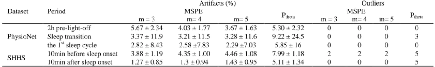
before further analysis. Table 3 summaries the artifacts and outliers excluded.
3.1 Analysis on Physionet dataset: MSPE gradually decreases and correlates with concomitant theta power towards light off
We first wondered whether MSPE would vary over the 2 hours preceding light off and correlate with concomitant Ptheta. To address this question, we used Physionet dataset as it contains > 2h of data
preceding light-off.
Figure 3A illustrates the average PE value (for all the participants) of each scale across the acquisition period before light off with embedding dimension m = 3 (the display obtained with m = 4
Accepted Manuscript
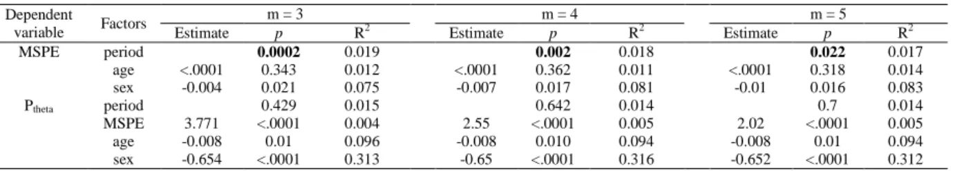
or 5 is similar; not shown here). Intuitively, the PE values at most of the scales fluctuate with a tendency of decreasing towards light-off. Figure 3B illustrated the MSPE values (mean±standard errors) obtained with m = 3, 4 or 5 and the lines were fitted with the averaged MSPE values across the acquisition periods. Progressive decline of MSPE towards light-off can be observed regardless of the value of m (Figure 3B; Mann-Kendall test, z = -10.9, -11.9 and -12.8 for m=3, 4 and 5, respectively, with p < 0.0001). GLMMs also show a significant change of MSPE with time (Table 4; main effect of acquisition period, p = 0.0002, 0.002 and 0.022 for m=3, 4 and 5, respectively). Moreover, at each time bin, MSPE value consistently decreases as m increases from 3 to 5 because the larger the embedding dimension, the more details are obtained from the signal; thus, less random the signal becomes and the smaller its MSPE value 64.
Similarly, an increase tendency towards light-off was observed in Ptheta (Mann-Kendall test, z =
5.88 and p < 0.0001; Figure 3C). After controlling for all confounding factors in a GLMM, no
significant effect of acquisition period on Ptheta was found (Table 4; GLMM, main effect of acquisition
period, p > 0.05). Moreover, in line with the literature 65, sex and age were significantly associated
with Ptheta with women showing higher theta power and theta power declining with age (Table 4;
GLMM, for sex and age, p < 0.0001 and p = 0.01, respectively, regardless of m). Importantly, Spearman’s correlation analyses over time bins indicate that Ptheta shows a significant positive link with MSPE for most time bins within 2h before light off (occurs at 227, 234 and 235 out 240 time bins for m=3, 4 and 5, respectively) (Figure 3D). Such a positive association is surprising given that, overall, both metrics evolve in opposite direction. GLMMs confirm however the significant positive association (Table 4; main effect of MSPE, p < 0.0001 regardless of m) after controlling for the effects of age and sex.
Furthermore, for each participant, we computed and compared the median values of MSPE during three periods of interest (Figure 2A), i.e, 2h before light-off, sleep transition after light-off, and the first sleep cycle. As the results obtained with m=3,4 or 5 are similar, only these with m=3 are displayed in Figure 4 which shows that MSPE gradually decrease from wakefulness to sleep transition and then to the first sleep cycle (Figure 4A). The results of ANOVA further indicate that
Accepted Manuscript
period is a main effect of MSPE (F = 332, p < 0.0001) and post-hoc analysis suggests there is significant difference between the MSPE values of each two periods. As for the concomitant Ptheta,
although ANOVA also indicates a significant effect of period (F = 35, p < 0.0001), only significant difference between the pre-light-off state and the sleep state was revealed (Figure 4B).
3.2 Analysis on SHHS dataset: MSPE decreases in wake-to-sleep transition and predicts sleep-onset
We then asked whether MSPE would vary during the transition from wake to sleep preceding sleep-onset (Figure 2B). To address this question, we switched to SHHS datasets as it includes many more subjects.
Figure 5A illustrates the average PE value for all the participants (m=3; the display is similar in
the situation of m=4 and 5; not shown) over each time bin within 10 minutes immediately before sleep onset. A progressive decline of PE towards sleep can be observed at scale one and two (Figure 5A). Although Mann-Kendall test only indicates significant decline of MSPE towards sleep in the situation of m=3 (Figure 5B; z = -3.34 and p <0.0001), GLMM analysis (Table 5) shows significant effect of acquisition period on MSPE (p < 0.05) regardless of m used. Likewise, significant decrease of Ptheta
with time was found (Figure 5C; Mann-Kendall test, z =-2.11 and p = 0.035; Table 5, GLMM, main effect of acquisition period, p < 0.05, regardless of m). Spearman’s correlation analyses over each time bin indicated significant negative association between Ptheta and MSPE for most of the time bins
and for all the embedding dimensions considered (Figure 5D). GLMMs confirmed that Ptheta was
significantly negatively associated to MSPE (Table 5; main effect of MSPE, p <0.001, regardless of m) including sex and age as covariates. The negative association comes again as a surprise given that, overall, both metrics evolve in the same direction in the transition to sleep (i.e. they both decrease).
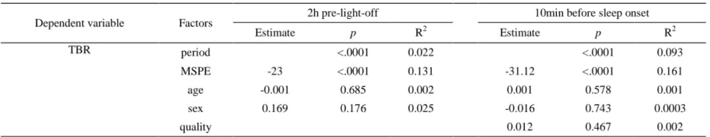
To investigate further the switch in correlation direction from pre-light-off wakefulness to the transition to sleep, we assesses the association between MSPE (m=3) and the ratio of EEG power in theta band and the fast beta frequency band (beta, 13-30Hz; theta/beta ratio, TBR). The analyses indicates that both during the 2h preceding light-off (Physionet dataset) and during the transition
Accepted Manuscript
towards sleep (SHHS dataset), the more theta, relative to faster frequencies, the lower the EEG signal complexity (Figure 6A-B, significant negative correlation between TBR and MSPE; Table 6, GLMM, main effect of MSPE, p <0.001).
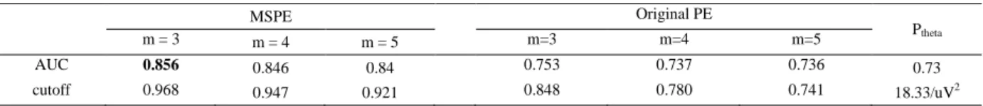
We finally focused on the ability of PE measures to discriminate between sleep and wakefulness around sleep onset. PE at different scales was found to have different ability to discriminate epochs before or after sleep onset (i.e., wake or sleep stages; Figure 7A) and excellent AUCs (more than 0.8) can be obtained at scales from 2 to 5 for all the embedding dimensions considered. Moreover, PEs calculated with a parameter m=3 outperforms those obtained with m=4 or 5 at all the scales. In the situation of m=3, PE of the original time series yielded to an acceptable AUC of 0.753, while the highest AUC, 0.870, was achieved at scale 4 (Figure 7A). We can also conclude from Figure 7B that MSPE with a parameter m=3 serves as the most discriminative method while the ROC of Ptheta is
nearest to the diagonal line. The AUC and cutoff values of the ROCs obtained by MSPE, PE of the original time series and Ptheta are further shown in Table 7, which indicates an obvious promotion of
discriminative ability with the application of multiscale analysis. In consistence with Figure 7B, an
excellent AUC of 0.856 was achieved by MSPE with m=3. However, the AUC was 0.730 when Ptheta
was used (Table 7), even less than those obtained by the PE values of the original time series.
4. DISCUSSION
Quantifying the complexity of the EEG signal during prolonged wakefulness and during sleep is gaining interest as an additional mean to characterize the mechanisms associated with sleep and wakefulness regulation. Here, we report significant changes in EEG complexity, as indexed by MSPE, immediately prior to light off and during the transition from wakefulness to sleep. We further report that MSPE can reach excellent (AUC > .8) discrimination between wakefulness and sleep around sleep onset and that MSPE changes are correlated with concomitant Ptheta spectral measures.
Accepted Manuscript
Standard Fast Fourier transformations (FFT) assume that the measured EEG signal consists in a linear combination of fluctuations of different frequencies. Brain oscillations are, however, not a linear combination of frequency components that could be added up. In other words, they are intrinsically nonlinear 17. Two main types of non-linear methods have been proposed to enrich the
characterization of the (sleep) EEG, fractal-based and entropy methods. Here, we used the latter type which measures the uncertainty about the information source and the probability distribution of the samples drawn from it, so that entropy can be an indicator of the complexity of the EEG signal 17. By
utilizing the recurrence of ordinal patterns in the signal, the calculation of PE takes into account time causality between the values of the time series and reflects the time characteristics of the underlying dynamics 19. A high PE value of scalp EEG signal was reported as a direct reflection of a more active
cortex with an EEG output which is less regular and exhibits higher frequency content 33. Entropy of
the sleep EEG has consistently been reported to gradually decrease from wake to sleep stage N1, N2 and N3, indicating that brain activity becomes less complex, more coherent and periodic, while entropy increases during REM as compare to NREM sleep 17, 64, 66, 67. Entropy likely decreases during
sleep because neurons are more synchronized (i.e., regular interactions within the neuronal network) 68
: frequency content slows down and amplitude increases, generating a less complex signal. The entropy decrease during NREM sleep could also arise from the fact that fewer neurons are involved in information processing. There are indeed several reports that brain signal remains more local during sleep with less interaction between distant brain regions 69, 70, and therefore potentially less neurons
contributing to the EEG signal. Here, we report that there is a decrease in MSPE during the 2h preceding light-off and in the transition from wakefulness to sleep, suggesting that, as for NREM sleep progression from N1 to N3 71, falling asleep is a gradual process. This is reminiscent of previous
intracranial recording in epileptic patients that detected spindles before sleep onset, particularly in the hippocampus 72. As for sleep, lower MSPE likely arises from a progressively more synchronized
neuronal activity. Whether reduced signal propagation also contributes is unclear as previous reports suggest that signal scattering increases in the evening before decreasing during nighttime wakefulness 73-75
.
Accepted Manuscript
Complexity measures have been used to differentiate conscious from unconscious states by quantifying the information content of the spatiotemporal cortical activity. Compared to wakefulness, reduced complexity was recorded during anesthesia, sleep and disorders of consciousness 76-78,
suggesting that complex brain activity is a prerequisite or a consequence of consciousness. Previous studies also demonstrated PE is maximal during wakefulness while decreases during sleep 64 and
tends to be greatest when the subjects are in fully alert states while falling in states with loss of awareness or consciousness 79. In line with these findings, we find that EEG complexity (or MSPE)
can effectively differentiate pre-sleep wakefulness, when computed over the 10 min preceding sleep-onset sleep-onset (defined as the first 2 consecutives epoch of N1 or N2 stages), from early sleep, when computed over the 10 min following sleep onset. It outperforms in fact theta band power in doing so. Furthermore, we show that MSPE decreases over the 2h preceding light off and over the 10 minutes preceding sleep (especially when m=3). Whether these changes reflect a progressive loss of
consciousness remains an open question. While one can posit that it is the case over the transition between sleep and wakefulness, it may be more difficult to argue that our sample of healthy participants was progressively less conscious before light-off.
We stress that any settings of MSPE computation could be used to efficiently track pre-sleep signal complexity changes. However, the results obtained from an embedding dimension of 3 and scale factor of 4 appear best for discriminating pre- and after- sleep-onset states. Future research will confirm whether the MSPE parameters (m=3, τ = 1 and maximal scales = 10) we used to be indeed the most effective to track pre-sleep EEG signal complexity alterations. We further emphasize that MSPE is an efficient method which is, in principle, more efficient than FFT. In computer science, an
algorithm with a time complexity of O(N), as MSPE, is considered to be more efficient than that with a time complexity of O(NlogN), such as FFT. In this respect, the MSPE has less computational cost than FFT. In practice, however, especially when N, representing the length of an EEG signal, is small (for example, less than 3000), the difference of the running times between both methods should be small.
Accepted Manuscript
Our explorations of the link with Ptheta shows that this well accepted spectral measure of sleep
need is significantly associated with MSPE. Yet, the link is puzzling. While MSPE and Ptheta evolve in
overall opposite direction over the 2h preceding light-off, their values are positively associated. In contrast in the transition to sleep, both metrics are globally decreasing and yet they are negatively correlated. Faster frequencies are progressively dominated by slower theta power during pre-light-off wakefulness as a reflection of the increase in sleep need 80. Our results suggest that during this period,
the more theta, relative to faster frequencies, the lower the EEG signal complexity. Following light-off, in the eye-closed transition toward sleep, the EEG further slows downs so that the dominant frequency likely lies in the theta/delta. This likely explains why our results show that during transition to sleep, the link with theta power switches to being negative. From a frequency analysis point of view, MSPE covers the entire spectrum of oscillations included in a time series, so one could consider it as a comprehensive measure that is not limited to a given frequency band and yet reflects a
progressive change brain state associated with sleep and wakefulness regulation.
We acknowledge that our study bears some limitations. First, as stated above, recording was ambulatory, thus providing less control over the experimental condition. We do not have information regarding the behavior of the participants, e.g. when they went to bed relative to light-off or the type of activities they were engaged in prior to going to bed. It is therefore unclear whether participants’ behavior may underlie part of the evolution of MSPE prior to light-off. This limitation may however constitute a strength: our findings are valid in real life situations. Second, artifacts in the data were not excluded following visual or validated automatic procedures, but were rather considered to be
efficiently removed by excluding sudden variations in MSPE or Ptheta within each recording. In
addition, while the current findings are based on large set of data in individuals devoid of sleep disorders (N=378), providing relatively high statistical sensitivity, MSPE may come with the cost of reduced sensitivity for some individual differences such as sex and age which are typically associated to EEG spectral analyses. Yet, MSPE significantly varied close to light-off and sleep onset,
particularly when setting the embedding dimension to 3. It may therefore constitute an entropy
Accepted Manuscript
approach more sensitive than others that previously failed to identify significant changes during in-lab sleep deprivation protocols 34, 74.
Modern society lifestyle often leads to sleep loss 81-83 and chronic sleep restriction 84 that cause
fatigue and impairment in vigilance, working memory, and cognitive throughput 85 and may lead to
accidents 86. MSPE is a low computation time method that may be an effective mean to detect when
the brain is in a state close to sleep onset.
Accepted Manuscript
Acknowledgments
This research was funded by the National Natural Science Foundation of China (Grant No.61401518 and 11974231) and the Double First‐ Class University project. GV is supported by FNRS (Belgium). GG was supported by Wallonia-Brussels International and ULiège.
The Sleep Heart Health Study was supported by the National Institutes of Health, National Heart Lung and Blood Institute (U01HL53916, U01HL53931, U01HL53934, U01HL53937, U01HL53938, U01HL53940, U01HL53941, U01HL64360). The National Sleep Research Resource was supported by the National Institutes of Health, National Heart Lung and Blood Institute (R24 HL114473, RFP 75N92019R002).
Disclosure Statement
Financial Disclosure: none.
Non-financial Disclosure: none.
Data Availability Statements
The data underlying this article are available at https://www.physionet.org/content/sleep-edfx/1.0.0/ and https://sleepdata.org/datasets/shhs/files/datasets .
Accepted Manuscript
References
1. Borbely AA, Achermann P. Sleep Homeostasis and Models of Sleep Regulation. Journal of Biological Rhythms 1999;14:557-68.
2. Giulio, Tononi, Chiara, Cirelli. Sleep and the Price of Plasticity: From Synaptic and Cellular Homeostasis to Memory Consolidation and Integration. Neuron 2014;81:12-34.
3. Borbély AA, Daan S, Wirz-Justice A, Deboer T. The two-process model of sleep regulation: a reappraisal. Journal of Sleep Research 2016;25:131-43.
4. Gaggioni G, Maquet P, Schmidt C, Dijk DJ, Vandewalle G. Neuroimaging, cognition, light and circadian rhythms. Front Syst Neurosci 2014;8:126.
5. Fattinger S, Kurth S, Ringli M, Jenni OG, Huber R. Theta waves in children's waking electroencephalogram resemble local aspects of sleep during wakefulness. Scientific Reports 2017;7:11187. 6. Holm A, Lukander K, Korpela J, Sallinen M, Müller KMI. Estimating brain load from the EEG. ScientificWorldJournal 2009;9:639-51.
7. Groppe DM, Bickel S, Keller CJ, et al. Dominant frequencies of resting human brain activity as measured by the electrocorticogram. NeuroImage 2013;79:223-33.
8. Borghini G, Astolfi L, Vecchiato G, Mattia D, Babiloni F. Measuring neurophysiological signals in aircraft pilots and car drivers for the assessment of mental workload, fatigue and drowsiness. Neuroscience and biobehavioral reviews 2014;44:58-75.
9. Kuo C-C, Lin WS, Dressel CA, Chiu AW. Classification of intended motor movement using surface EEG ensemble empirical mode decomposition. In: 2011 Annual International Conference of the IEEE Engineering in Medicine and Biology Society 2011; 2011:6281-4.
10. Wascher E, Getzmann S, Karthaus M. Driver state examination--Treading new paths. Accid Anal Prev 2016;91:157-65.
11. Budi, Thomas, Jap, et al. Using EEG spectral components to assess algorithms for detecting fatigue. Expert Systems with Applications 2009;36:2352-9.
12. Jagannath M, Balasubramanian V. Assessment of early onset of driver fatigue using multimodal fatigue measures in a static simulator. Applied Ergonomics 2014;45:1140-7.
13. Foong R, Kai KA, Chai Q, Guan C, Wai AAP. An Analysis on Driver Drowsiness Based on Reaction Time and EEG Band Power. In: 37TH ANNUAL INTERNATIONAL CONFERENCE OF THE IEEE Engineering in Medicine and Biology Society; 2015, 2015:7982-5.
14. Mahachandra M, Garnaby ED. The effectiveness of in-vehicle peppermint fragrance to maintain car driver's alertness. Procedia Manufacturing 2015;4:471-7.
15. Natarajan K, Rajendra AU, Alias F, Tiboleng T, Puthusserypady SK. Nonlinear analysis of EEG signals at different mental states. Biomedical Engineering Online 2004;3:7.
16. Yin Y, Shang P. Multivariate weighted multiscale permutation entropy for complex time series. Nonlinear Dynamics 2017;88:1707-22.
17. Ma Y, Shi W, Peng C-K, Yang AC. Nonlinear dynamical analysis of sleep electroencephalography using fractal and entropy approaches. Sleep medicine reviews 2018;37:85-93.
18. Zanin, Massimiliano, Zunino, et al. Entropy, Vol. 14, Pages 1553-1577: Permutation Entropy and Its Main Biomedical and Econophysics Applications: A Review. 2012;14:1553-77.
19. Bandt C, Pompe B. Permutation Entropy: A Natural Complexity Measure for Time Series. Physical Review Letters 2002;88:174102.
20. Groth A. Visualization of coupling in time series by order recurrence plots. Physical Review E 2005;72:046220.
21. Olofsen E, Sleigh JW, Dahan A. Permutation entropy of the electroencephalogram: a measure of anaesthetic drug effect. Br J Anaesth 2008;101:810-21.
22. Cao Y, Tung WW, Gao JB, Protopopescu VA, Hively LM. Detecting dynamical changes in time series using the permutation entropy. Phys Rev E Stat Nonlin Soft Matter Phys 2004;70:046217.
23. Keller K, Wittfeld K. Distances of time series components by means of symbolic dynamics. International Journal of Bifurcation and Chaos 2004;14:693-703.
24. Li X, Ouyang G, Richards DA. Predictability analysis of absence seizures with permutation entropy. Epilepsy research 2007;77:70-4.
25. Ouyang G, Dang C, Richards DA, Li X. Ordinal pattern based similarity analysis for EEG recordings. Clinical Neurophysiology 2010;121:694-703.
26. Olofsen E, Sleigh J, Dahan A. Permutation entropy of the electroencephalogram: a measure of
Accepted Manuscript
anaesthetic drug effect. British journal of anaesthesia 2008;101:810-21.27. Silva A, Campos S, Monteiro J, et al. Performance of Anesthetic Depth Indexes in Rabbits under Propofol AnesthesiaPrediction Probabilities and Concentration-effect Relations. Anesthesiology: The Journal of the American Society of Anesthesiologists 2011;115:303-14.
28. Silva A, Cardoso-Cruz H, Silva F, Galhardo V, Antunes L. Comparison of anesthetic depth indexes based on thalamocortical local field potentials in rats. Anesthesiology 2010;112:355.
29. Schinkel S, Marwan N, Kurths J. Order patterns recurrence plots in the analysis of ERP data. Cognitive Neurodynamics 2007;1:317-25.
30. Schinkel S, Marwan N, Kurths J. Brain signal analysis based on recurrences. J Physiol Paris 2009;103:315-23.
31. Thul A., ;Lechinger J., Donis J. et al. EEG entropy measures indicate decrease of cortical information processing in Disorders of Consciousness. Clinical Neurophysiology 2016;127:1419-27.
32. Wielek T, Lechinger J, Wislowska M, et al. Sleep in patients with disorders of consciousness characterized by means of machine learning. PLoS ONE 2018;13:1-14.
33. Nicolaou N, Georgiou J. The Use of Permutation Entropy to Characterize Sleep Electroencephalograms. Clinical Eeg & Neuroscience Official Journal of the Eeg & Clinical Neuroscience Society 2011;42:24-8.
34. Tosun PD, Dijk D-J, Winsky-Sommerer R, Abasolo D. Effects of ageing and sex on complexity in the human sleep EEG: A comparison of three symbolic dynamic analysis methods. Complexity 2019;2019.
35. Linkenkaer-Hansen K, Nikouline VV, Palva JM, Ilmoniemi RJ. Long-range temporal correlations and scaling behavior in human brain oscillations. The Journal of neuroscience : the official journal of the Society for Neuroscience 2001;21:1370-7.
36. Smith RJ, Sugijoto A, Rismanchi N, Hussain SA, Shrey DW, Lopour BA. Long-Range Temporal Correlations Reflect Treatment Response in the Electroencephalogram of Patients with Infantile Spasms. Brain Topogr 2017;30:810-21.
37. Costa M, Goldberger AL, Peng CK. Multiscale entropy analysis of complex physiologic time series. Phys Rev Lett 2002;89:068102.
38. Costa M, Goldberger AL, Peng CK. Multiscale entropy analysis of biological signals. Phys Rev E Stat Nonlin Soft Matter Phys 2005;71:021906.
39. Liu Q, Chen Y-F, Fan S-Z, Abbod MF, Shieh J-S. EEG Signals Analysis Using Multiscale Entropy for Depth of Anesthesia Monitoring during Surgery through Artificial Neural Networks. Comput Math Methods Med 2015;2015:232381.
40. Chen C, Li J, Lu X. Multiscale entropy-based analysis and processing of EEG signal during watching 3DTV. Measurement 2018;125:432-7.
41. Lu W-Y, Chen J-Y, Chang C-F, Weng W-C, Lee W-T, Shieh J-S. Multiscale Entropy of Electroencephalogram as a Potential Predictor for the Prognosis of Neonatal Seizures. PLoS One 2015;10:0144732.
42. Norris PR, Anderson SM, Jenkins JM, Williams AE, Morris Jr JA. Heart rate multiscale entropy at three hours predicts hospital mortality in 3,154 trauma patients. Shock 2008;30:17-22.
43. Silva LEV, Lataro RM, Castania JA, et al. Multiscale entropy analysis of heart rate variability in heart failure, hypertensive, and sinoaortic-denervated rats: classical and refined approaches. American Journal of Physiology-Regulatory, Integrative and Comparative Physiology 2016;311:150-6.
44. Udhayakumar RK, Karmakar C, Palaniswami M. Multiscale entropy profiling to estimate complexity of heart rate dynamics. Physical Review E 2019;100:012405.
45. Zhijun, Yao, Yuanchao, et al. Abnormal Cortical Networks in Mild Cognitive Impairment and Alzheimer's Disease. Plos Computational Biology 2010;11:1001006.
46. Mourtazaev MS, Kemp B, Zwinderman AH, Kamphuisen HAC. Age and Gender Affect Different Characteristics of Slow Waves in the Sleep EEG. Sleep 1995;18:557.
47. Zhang GQ, Cui L, Mueller R, et al. The National Sleep Research Resource: towards a sleep data commons. J Am Med Inform Assoc 2018;25:1351-8.
48. Quan SF, Howard BV, Iber C, et al. The Sleep Heart Health Study: design, rationale, and methods. Sleep 1997;20:1077-85.
49. Thomas RJ, Mietus JE, Peng CK, et al. Differentiating Obstructive from Central and Complex Sleep Apnea Using an Automated Electrocardiogram-Based Method. Sleep 2007;30:1756.
50. https://sleepdata.org/datasets/shhs/variables/overall_shhs1.
51. Duhamel P, Vetterli M. Fast Fourier transforms: a tutorial review and a state of the art. Signal Processing (Elsevier) 1990;19:259-99.
52. Viola AUa, Archer SNa, b, James La, et al. PER3 Polymorphism Predicts Sleep Structure and Waking
Accepted Manuscript
Performance(Article). Current Biology 2007:613-8.53. Ly JQM, Gaggioni G, Chellappa SL, et al. Circadian regulation of human cortical excitability. Nature Communications 2016;7:11828.
54. Cajochen C, Wyatt JK, Czeisler CA, Dijk DJ. Separation of circadian and wake duration-dependent modulation of EEG activation during wakefulness. Neuroscience 2002;114:1047-60.
55. Rétey JV, Adam M, Gottselig JM, et al. Adenosinergic mechanisms contribute to individual differences in sleep deprivation-induced changes in neurobehavioral function and brain rhythmic activity. The Journal of neuroscience : the official journal of the Society for Neuroscience 2006;26:10472-9.
56. Finelli LA, Baumann H, Borbly AA, Achermann P. Dual electroencephalogram markers of human sleep homeostasis: correlation between theta activity in waking and slow-wave activity in sleep. Neuroscience 2000:523-9.
57. Hung C, Sarasso S, Ferrarelli F, et al. Local experience-dependent changes in the wake EEG after prolonged wakefulness. Sleep 2013:59-72.
58. Feinberg I, Floyd TC. Systematic Trends Across the Night in Human Sleep Cycles. Psychophysiology 2010;16:283-91.
59. Mandrekar JN. Receiver operating characteristic curve in diagnostic test assessment. Journal of thoracic oncology : official publication of the International Association for the Study of Lung Cancer 2010;5:1315-6.
60. Youden WJ. Index for rating diagnostic tests. Cancer 1950;3:32-5.
61. Zar JH. Significance Testing of the Spearman Rank Correlation Coefficient. Publications of the American Statistical Association 1972;67:578-80.
62. Mann HB. Non-Parametric Test Against Trend. Econometrica 1945;13:245-59.
63. Kenward MG, Roger JH. Small Sample Inference for Fixed Effects from Restricted Maximum Likelihood. Biometrics 1997;53:983-97.
64. González J, Cavelli M, Mondino A, et al. Decreased electrocortical temporal complexity distinguishes sleep from wakefulness. Scientific Reports 2019;9:18457.
65. Carrier J, Semba K, Deurveilher S, et al. Sex differences in age-related changes in the sleep-wake cycle. Frontiers in neuroendocrinology 2017;47:66-85.
66. Fell J, Röschke J, Mann K, Schäffner C. Discrimination of sleep stages: a comparison between spectral and nonlinear EEG measures. Electroencephalography and clinical Neurophysiology 1996;98:401-10.
67. Achermann P, Hartmann R, Gunzinger A, Guggenbüh W, Borbély AA. Correlation dimension of the human sleep electroencephalogram: cyclic changes in the course of the night. European Journal of Neuroscience 1994;6:497-500.
68. Steriade M. The corticothalamic system in sleep. Frontiers in bioscience: a journal and virtual library 2003;8:d878-99.
69. Massimini M, Ferrarelli F, Huber R, Esser SK, Singh H, Tononi G. Breakdown of cortical effective connectivity during sleep. Science 2005;309:2228-32.
70. Boly M, Perlbarg V, Marrelec G, et al. Hierarchical clustering of brain activity during human nonrapid eye movement sleep. Proceedings of the National Academy of Sciences 2012;109:5856-61.
71. Colton H, Altevogt B. Sleep disorders and sleep deprivation: an unmet public health problem. In: Washington, DC: National Academies Press, 2006.
72. Sarasso S, Proserpio P, Pigorini A, et al. Hippocampal sleep spindles preceding neocortical sleep onset in humans. Neuroimage 2014;86:425-32.
73. Meisel C, Klaus A, Vyazovskiy VV, Plenz D. The interplay between long-and short-range temporal correlations shapes cortex dynamics across vigilance states. Journal of neuroscience 2017;37:10114-24. 74. Gaggioni G, Ly JQ, Chellappa SL, et al. Human fronto-parietal response scattering subserves vigilance at night. Neuroimage 2018;175:354-64.
75. Meisel C, Bailey K, Achermann P, Plenz D. Decline of long-range temporal correlations in the human brain during sustained wakefulness. Scientific reports 2017;7:1-11.
76. Rathee D, Cecotti H, Prasad G. (Un) Consciousness and Time-Series Complexity A study with spontaneous EEG. In: MEG UK 2016; 2016.
77. Thul A, Lechinger J, Donis J, et al. EEG entropy measures indicate decrease of cortical information processing in Disorders of Consciousness. Clinical neurophysiology : official journal of the International Federation of Clinical Neurophysiology 2016;127:1419-27.
78. Wielek T, Lechinger J, Wislowska M, et al. Sleep in patients with disorders of consciousness characterized by means of machine learning. PLoS One 2018;13:0190458.
79. Mateos DM, Guevara Erra R, Wennberg R, Perez Velazquez JL. Measures of entropy and complexity in
Accepted Manuscript
altered states of consciousness. Cognitive Neurodynamics 2018;12:73-84.80. Cajochen DC, Dijk D-J. Electroencephalographic activity during wakefulness, rapid eye movement and non-rapid eye movement sleep in humans: Comparison of their circadian and homeostatic modulation. Sleep and Biological Rhythms 2003;1:85-95.
81. Basner M, Rao H, Goel N, Dinges DF. Sleep deprivation and neurobehavioral dynamics. Current opinion in neurobiology 2013;23:854-63.
82. Killgore WD. Effects of sleep deprivation on cognition. Progress in brain research: Elsevier, 2010:105-29.
83. Durmer JS, Dinges DF. Neurocognitive consequences of sleep deprivation. Seminars in neurology 2005;25: 117-29.
84. Maric A, Lustenberger C, Werth E, Baumann CR, Poryazova R, Huber R. Intraindividual increase of homeostatic sleep pressure across acute and chronic sleep loss: A high-density eeg study. Sleep 2017;40:122. 85. Siobhan B, Dinges DF. Behavioral and physiological consequences of sleep restriction. Journal of Clinical Sleep Medicine Jcsm Official Publication of the American Academy of Sleep Medicine 2007;3:519. 86. Wascher E, Getzmann S, Karthaus M. Driver state examination—Treading new paths. Accid Anal Prev 2016;91:157-65.
Accepted Manuscript
Figure Captions
Figure 1. (color online) Illustration of the MSPE algorithm. (A) the coarse-graining procedure for scale
factor of 3. Each black dot represents a data point in the original time series. (B) the ordinal patterns in MSPE calculation with embedding dimension of 4 and time lag of 1. The circle dots in (B) represent the data points in a time series, and the combination of four numbers under a rectangle or a horizontal line stands for an ordinal pattern of the segment in the rectangle or right above the line. The segments in the rectangles have the same pattern [2, 3, 1, 4].
Figure 2. Schematic diagram of the timeline in the analyses. (A) The timeline for the analysis on PhysioNet
dataset. MSPE and Ptheta were evaluated in three different periods, i.e., 2h pre-light-off, the sleep transition from
light-off to sleep onset, and the first sleep cycle. (B) The timeline for the analysis on SHHS dataset. The included subjects must have a sleep latency more than 10 minutes. MSPE and Ptheta were computed over each
30s epoch within the 10 minutes immediately preceding and following sleep onset.
Figure 3. (color online) Variations in MSPE and Ptheta values before light off. (A) Average value of PE for
all the participants in PhysioNet datasets using different scale factors. For the calculation of PE, the embedding dimension m was set as 3. (B) Average MSPE at m = 3, 4 or 5 at each time bin; shade areas represent the standard errors of the mean. (C) Average Ptheta at each time bin; shade areas represent the standard errors of the
mean. (D) p-values of the Spearman correlation between MSPE (with m set as 3, 4 or 5) and concomitant Ptheta
over each time bin.
Figure 4. The values of MSPE (A) and Ptheta (B) during pre-light-off wakefulness, pre-sleep wakefulness
and 1st sleep NREM-REM cycle. Each dot represents the median value of MSPE or Ptheta for a participant
during the corresponding period. The box-plots illustrate the distributes of these median values for all the participants in PhysioNet dataset. The symbol ‘*’ represents for a significant difference of median values between groups (post-hoc tests of ANOVA, p<0.05).
Figure 5. (color online) Variations in MSPE and Ptheta values within 10 minutes immediately before
sleep-onset. (A) Average value of PE for all the participants in PhysioNet datasets using different scale factors. For
the calculation of PE, the embedding dimension m was set as 3. (B) Average MSPE at m = 3, 4 or 5 at each time bin; shade areas represent the standard errors of the mean. (C) Average Ptheta at each time bin; shade areas
represent the standard errors of the mean. (D) p-values of the Spearman correlation between MSPE (with m set as 3, 4 or 5) and concomitant Ptheta over each time bin.
Figure 6. (color online) The Spearman's rho and its p-value between MSPE and TBR during (A)
the 2h pre-light-off with PhysioNet dataset and (B) the 10min before sleep-onset with SHHS dataset. Here, m was set as 3 in the calculation of MSPE and TBR represents the ratio of EEG power in theta band and beta band.
Figure 7. (color online) The AUC values to differentiate states before and after sleep-onset. (A) AUC
values of PE obtained with different scale factors and different embedding dimensions (3, 4 or 5). AUC values above the dashed line corresponds to an excellent ability of the test. (B) ROC curves of Ptheta and MSPE obtained
with m = 3, 4 or 5.
Accepted Manuscript
Tables
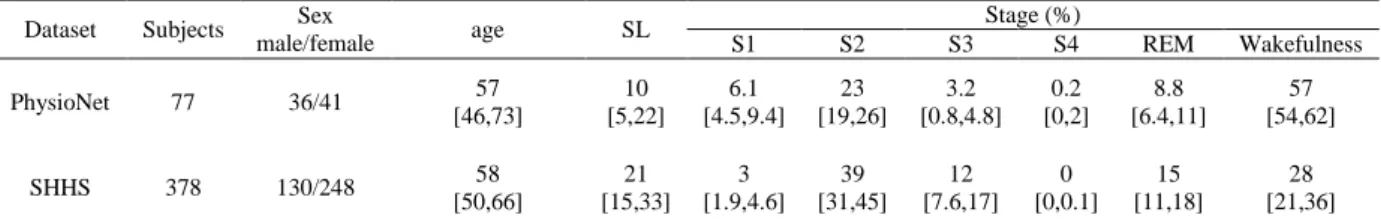
Table 1. Demographics and sleep structures of the included subjects. Dataset Subjects Sex
male/female age SL Stage (%) S1 S2 S3 S4 REM Wakefulness PhysioNet 77 36/41 57 [46,73] 10 [5,22] 6.1 [4.5,9.4] 23 [19,26] 3.2 [0.8,4.8] 0.2 [0,2] 8.8 [6.4,11] 57 [54,62] SHHS 378 130/248 58 [50,66] 21 [15,33] 3 [1.9,4.6] 39 [31,45] 12 [7.6,17] 0 [0,0.1] 15 [11,18] 28 [21,36] Note: Values are expressed as median [lower quartile, upper quartile]. Abbreviations: SL, Sleep latency; S1, Stage 1 of NREM sleep; S2, Stage 2 of NREM sleep; S3, Stage 3 of NREM sleep; S4, Stage 4 of NREM sleep; REM, Rapid Eye Movement; SHHS, the Sleep Heart Health Study.
Accepted Manuscript
Table 2. A pseudocode of the MSPE algorithm [Entropy] = MSPE(N, S, m, tau)
% N is the data length of the original signal, S is the maximal scale, m is the embedding dimension, and tau is the lag Entropy = 0
for ( i = 1 : S ) % treat the ith coarse-grained time series
for ( j = 1 : (N/i – (m-1)) * tau) ) % process the jth m-dimensional vector % sort the vector with a lowest computational complexity of O(mlogm)
% increase the count for its corresponding pattern with a computational complexity of O(1) PE = 0 % the PE value of the ith coarse-grained time series
for ( k = 1: m! ) % calculate the Shannon_entropy of all the possible patterns % calculate - p(k) * log(k) and add it to PE with a computational complexity of O(1) % normalize PE with a computational complexity of O(1)
Entropy = Entropy + PE
Entropy = Entropy / S % multiple-scales average
Accepted Manuscript
Table 3. Artifacts and outliers detected for the periods of interest in both datasets, based on MSPE or Ptheta values.
Dataset Period
Artifacts (%) Outliers
MSPE
Ptheta MSPE Ptheta
m = 3 m= 4 m= 5 m = 3 m= 4 m= 5
PhysioNet
2h pre-light-off 5.67 ± 2.34 4.03 ± 1.77 3.67 ± 1.63 5.30 ± 2.32 0 0 0 0 Sleep transition 3.37 ± 11.9 3.21 ± 11.5 3.28 ± 11.6 9.22 ± 24.5 0 0 0 3 the 1st sleep cycle 2.82 ± 8.43 2.58 ±7.83 2.29 ±7.03 5.85 ± 16 0 0 0 0 SHHS 10min before sleep onset 3.88 ± 1.19 4.35 ± 1.00 4.46 ± 1.08 7.99 ± 1.18 2 2 2 5 10min after sleep onset 1.27 ± 0.85 1.3 ± 0.94 1.43 ± 0.95 5.11 ± 1.34 0 0 0 5
Accepted Manuscript
Table 4. Results of GLMM evaluating the association between acquisition periods preceding light off and MSPE or Ptheta.
Dependent
variable Factors
m = 3 m = 4 m = 5
Estimate p R2 Estimate p R2 Estimate p R2
MSPE period 0.0002 0.019 0.002 0.018 0.022 0.017 age <.0001 0.343 0.012 <.0001 0.362 0.011 <.0001 0.318 0.014 sex -0.004 0.021 0.075 -0.007 0.017 0.081 -0.01 0.016 0.083 Ptheta period 0.429 0.015 0.642 0.014 0.7 0.014 MSPE 3.771 <.0001 0.004 2.55 <.0001 0.005 2.02 <.0001 0.005 age -0.008 0.01 0.096 -0.008 0.010 0.094 -0.008 0.01 0.094 sex -0.654 <.0001 0.313 -0.65 <.0001 0.316 -0.652 <.0001 0.312
Accepted Manuscript
Table 5. Results of GLMM evaluating the association between acquisition periods preceding sleep onset and MSPE or Ptheta.
Dependent
variable Factors
m = 3 m = 4 m = 5
Estimate p R2 Estimate p R2 Estimate p R2
MSPE period 0.0001 0.008 0.016 0.006 0.02 0.005 age <.0001 0.116 0.007 <.0001 0.072 0.009 0.0001 0.082 0.009 sex -0.0004 0.598 0.001 -0.0009 0.494 0.001 -0.001 0.453 0.002 quality <.0001 0.969 <.0001 -0.0001 0.762 0.003 -0.0004 0.521 0.001 Ptheta period 0.039 0.005 0.012 0.006 0.007 0.006 MSPE -16.50 <.0001 0.054 -10.76 <.0001 0.063 -9.08 <.0001 0.073 age -0.001 0.575 0.001 -0.001 0.602 0.0008 -0.001 0.596 0.001 sex 0.05 0.463 0.0014 0.046 0.492 0.001 0.044 0.513 0.001 quality -0.024 0.33 0.003 -0.025 0.302 0.003 -0.026 0.28 0.003
Accepted Manuscript
Table 6. Results of GLMM evaluating the association between MSPE (m=3) and TBR during two periods.
Dependent variable Factors 2h pre-light-off 10min before sleep onset
Estimate p R2 Estimate p R2 TBR period <.0001 0.022 <.0001 0.093 MSPE -23 <.0001 0.131 -31.12 <.0001 0.161 age -0.001 0.685 0.002 0.001 0.578 0.001 sex 0.169 0.176 0.025 -0.016 0.743 0.0003 quality 0.012 0.467 0.002
TBR: the ratio of EEG power in theta band and beta band.
Accepted Manuscript
Table 7. The AUC and cutoff values of MSPE and original PE obtained with m = 3, 4, or 5 and of Ptheta.
MSPE Original PE
Ptheta
m = 3 m = 4 m = 5 m=3 m=4 m=5
AUC 0.856 0.846 0.84 0.753 0.737 0.736 0.73
cutoff 0.968 0.947 0.921 0.848 0.780 0.741 18.33/uV2
Accepted Manuscript
Figure 1
Accepted Manuscript
Figure 2
Accepted Manuscript
Figure 3
Accepted Manuscript
Figure 4
Accepted Manuscript
Figure 5
Accepted Manuscript
Figure 6
Accepted Manuscript
Figure 7