HAL Id: hal-01166589
https://hal.archives-ouvertes.fr/hal-01166589
Submitted on 23 Jun 2015
HAL is a multi-disciplinary open access
archive for the deposit and dissemination of
sci-entific research documents, whether they are
pub-lished or not. The documents may come from
teaching and research institutions in France or
abroad, or from public or private research centers.
L’archive ouverte pluridisciplinaire HAL, est
destinée au dépôt et à la diffusion de documents
scientifiques de niveau recherche, publiés ou non,
émanant des établissements d’enseignement et de
recherche français ou étrangers, des laboratoires
publics ou privés.
A NEW APPROACH FOR THE BEST-CASE
SCHEDULE IN A GROUP SEQUENCE
Zakaria Yahouni, Nasser Mebarki, Zaki Sari
To cite this version:
Zakaria Yahouni, Nasser Mebarki, Zaki Sari. A NEW APPROACH FOR THE BEST-CASE
SCHED-ULE IN A GROUP SEQUENCE . MOSIM 2014, 10ème Conférence Francophone de Modélisation,
Optimisation et Simulation, Nov 2014, Nancy, France. �hal-01166589�
A NEW APPROACH FOR THE BEST-CASE SCHEDULE IN A
GROUP SEQUENCE
Zakaria YAHOUNI1,2 , Nasser MEBARKI1 , Zaki SARI2 1LUNAM, Universit´e de Nantes, 2MELT
IRCCyN, Institut de Recherche en Communications
Manufacturing Engineering Laboratory
et Cybern´etique de Nantes, UMR CNRS 6597
of tlemcen
Nantes - France Tlemcen - Algeria
[email protected] zaki [email protected]
ABSTRACT: The job-shop scheduling problem is an NP-hard optimization problem. It is generally solved using either predictive methods such as discrete optimization which try to find a solution that fits constraints and that optimizes one or more objectives or using reactive methods such real-time control methods which try to build incrementally in real-time a solution of the problem. Predictive-reactive methods try to combine both advantages of predictive and reactive methods (i.e., good performances and reactivity). The group sequencing method is one of the most studied predictive-reactive methods. The goal of this method is to have a sequential flexibility during the execution of the schedule and to guarantee a minimal quality corresponding to the worst-case.The best-case quality has also been successfully addressed by Pinot (2008) using a branch and bound procedure. It has been established for every regular objective. In this paper we propose two new branching processes to compute the best-case for the makespan which is one of the most studied regular objective. The experiments made on very well-known instances of the job-shop problem show the benefits of these new branching procedures.
KEYWORDS: JobShop, Group Sequence, Branch and Bound, Makespan, Best-case, Flexibility .
1 INTRODUCTION
The job shop problem with precedence constraints and release date is a classical scheduling situation (J/ri,Pred/f according to the classification of Graham et al. (1979)), where ji denotes the job number i and every job is composed of one or many operations O0, O1, .... Oj−1, Oj where Oj−1 is the precedence operation of Oj and in contrast Oj is the successor of Oj−1(denoted as Γ− and Γ+ resp.), an operation Oi has a release date ri, a starting time ti, an execution time pi and a completion time Ci, each operation needs to be executed on a resource called machine Mk (each machine executes only one operation at a time), f being an objective function, the objective treated. In this paper we adress only the makespan which is a classical regular objective. The makespan corresponds to the total time of the schedule execution, denoted Cmax.
Predictive modeling techniques are a classical solution for a job shop problem where all data and parame-ters of the problem are assumed to be fully known. However, in practice, manufacturing problems are not always deterministic, many disturbances can occur during the execution of the schedule which change
the data of the initial problem. These disturbances will, in most cases, deteriorate the expected perfor-mances. The workaround for this problem requires the development of a new robust and flexible solution that takes into account the uncertainties of the workshop. Three approaches are proposed and studied in the lit-erature for scheduling under uncertainties Davenport and Beck (2000). The first ones are proactive methods that treat uncertainties only in the static phase of the overall process of the resolution, the second methods are called reactive methods that work symmetrically to the proactive ones, this approach manages uncer-tainties during the dynamic phase in real-time with the scheduling process and does not benefit from the advantages that provide the proactive methods. Proactive-Reactive methods benefit from both ad-vantages of the previous approaches, they take into account flexibility during the offline and the online phases; in the static phase they build a flexible solu-tion to ensure a certain performance while responding to unexpected events during the resolution phase. For a detail information about this three approaches see Esswein (2003).
One of the most famous proactive-reactive methods is the group sequence method that was created by Er-schler and Roubellat (1989). This method is composed
10th International Conference of Modeling and Simulation - MOSIM14 November 5-7 - Nancy - France
of two phases:
• A predictive phase which aims at computing a solution offline. This solution is a set of schedules.
• A reactive phase in which a schedule is realized on-line in the shop. This phase relies on the solution proposed during the predictive phase and takes into account the real state of the shop. Thus, the schedule which is realized takes into account the uncertainties which occur in the shop.
This method aims at describing a set of feasible sched-ules in order to delay decisions to take into account uncertainties and evaluates a group sequence accord-ing to the worst-case quality in the set of feasible schedules. This approach has been widely studied in the past years Esswein (2003); Aloulou and Artigues (2007); Artigues et al. (2005); Pinot et al. (2007, 2009); Pinot and Mebarki (2009); Logendran et al. (2005); Cardin et al. (2013).
Esswein (2003); Artigues et al. (2005) proved that the worst-case quality of a group sequence can be computed in a polynomial time for regular min-max objectives, this criterion is very helpful to evaluate a decision during the execution of the schedule. How-ever, the best-case quality of a group sequence can also be interesting by providing to the decision maker two bounds, i.e., the minimal and the maximal quality of the schedule (Zworstand Zbest resp.)Mebarki et al. (2013). The computation of the best-case quality is based on the lower bounds proposed by Pinot and Mebarki (2008). These lower bounds are very inter-esting because they can be computed in polynomial time and they are used in a branch and bound algo-rithm used to compute the exact value of the best-case quality of any regular objective. Very good results were obtained but the method is very sensible to the branching process. To improve the branching proce-dure, we propose two new branching procedures for the makespan, which is one of the most used criteria to schedule jobs in a shop. The results show the ef-ficiency of these methods regarding the one used by Pinot and Mebarki (2009).
This paper is organized as follows: second section gives a brief definition with an example of the group sequence method. Section three describes the branch and bound method for the best-case in a group se-quence method, in section four and five, we propose our contribution, by proposing two techniques for the branching process in the branch and bound algorithm for the best-case schedule in a group sequence, then we present the experimentations made. The last two sections include the discussion of the results obtained and the conclusion.
2 GROUP SEQUENCE
Group of permutable operations was introduced by LAAS-CNRS laboratory, Toulouse, France Erschler and Roubellat (1989), this approach has been used in the ORDO software. The objective of this method is to provide to the decision-maker a sequential flexibility during the execution of the schedule and to ensure a certain quality that is represented by the worst process case.
A group of permutable operations is composed of groups Gi (or Gl,kwhere k is the machine index and l is the index of the group in the machine k), each group contains one or many operations that will be executed in the same resource Gi:={O1, O2, .., On}, n is the number of operations in the group Gi, n! is the number of permutations that can be concluded from this group. A group of permutable operations is said feasible if any permutation among all the operations of the same group gives a feasible schedule that satisfies all the constraints of the problem. As a matter of fact, a group sequence describes a set of valid schedules, without enumerating them.
The quality of a group sequence is expressed in the same way as that a classical schedule, it is measured as the quality of the worst semi-active schedule found in the group sequence as defined in Aloulou and Artigues (2007).
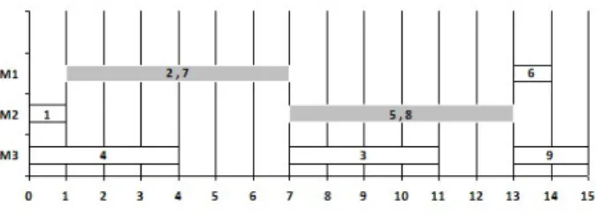
To illustrate this definition, let us study an example where the problem is described in tab 1.
ji j1 j2 j3
Oi 1 2 3 4 5 6 7 8 9
Mk M2 M1 M3 M3 M2 M1 M1 M2 M3
pi 1 4 4 4 3 1 2 3 2
Table 1: Example of a Job shop problem
Figure 1: Group Schedule
Tab. 1 presents a job shop problem with three ma-chines and three jobs, while Figure 1 represents a feasible group sequence solving this problem. This group sequence is made of seven groups: two groups of two operations and five groups of one operation. This group sequence describes four different semi-active
schedules shown in Figure 2. Note that these sched-ules do not always have the same makespan: the best-case quality is with Cmax=12 and the worst-case quality is with Cmax=14.
Figure 2: Enumeration of the semi-active schedules
The execution of a group sequence consists in choosing a particular schedule among the different possibilities described by the group sequence. It can be viewed as a sequence of decisions: each decision consists in choosing an operation to execute in a group when this group is composed of two or more operations. For instance, for the group sequence described on Figure 1, there are two decisions to be taken: on M1, at the beginning of the scheduling, either operation O2or O7 has to be executed. Let us suppose the decision taken is to schedule O2 before O7, on M2, there is another decision: scheduling operation O5 or O8 first, so at the end we have four semi-active schedules.
Group sequencing has an interesting property: the quality of a group sequence in the worst-case can be computed in polynomial time for minmax regular objective functions like makespan (Esswein (2003); Artigues et al. (2005); Aloulou and Artigues (2007). Thus, it is possible to compute the worst-case quality for large scheduling problems. Consequently, this method can be used to compute the worst-case quality in real-time during the execution of the schedule. Due to this property, it is possible to use group sequencing in a decision support system in real-time during the execution of the scheduling process.
This method enables the description of a set of sched-ules in an implicit manner (i.e. without enumerating the schedules) and guarantees a minimal performance that corresponds to worst-case quality. But the best-case quality should also be interesting to know which operation to chose from a current group to get possibly the best schedule.
3 BRANCH AND BOUND APPROACH FOR THE BEST-CASE IN A GROUP SE-QUENCE
Pinot and Mebarki (2009) have proposed a branch and bound algorithm to compute the best case quality in a group sequence. This algorithm relies on lower bounds proposed by Pinot and Mebarki (2008) 3.1 Lower bounds
The lower bounds are computed using a relaxation on the resources by making the assumption that each resource has an infinite capacity. In this case, the best-case lower bound for starting time of an operation (θi) is computed as the maximum of the best-case (lower bound) completion time (χj) of all its predecessors: for an operation Oi , its predecessors include the predecessors given by the problem (Γ−(i)) but also the operations on the previous group on the same machine (g−(i) being the predecessor group of g(i) on the same machine). Pinot and Mebarki (2008) improved these lower bounds by using a property of group-sequencing: an operation in a given group cannot be executed until all the execution of all the operations of its previous group. As a consequence, an operation can only begin after the optimal makespan of the previous group. It needs the computation of the optimal makespan of a group (named as γgl,k) which
is polynomially solvable by ordering the operations in ascending release date(θi) (Brucker and Knust (2008); Lawler (1973)).
The improved lower bounds are presented in equation1, and the lower bound of the example presented in tab. 1 is given in tab. 2:
θi= max(ri, γg−(i),max
| {z }
j∈Γ− (i)
χj)
χi= θi+ ρi
γgl,k = Cmax1|ri|Cmax, ∀Oi ∈ gl,k, ri= θi
(1) Oi θi χi 1 0 1 4 0 4 7 0 2 2 1 5 8 2 5 5 4 7 6 7 8 3 5 9 9 9 11
10th International Conference of Modeling and Simulation - MOSIM14 November 5-7 - Nancy - France
3.2 Branch and Bound algorithm
Every operation on each group will be represented by a node on the search space, A solution is an ordered sequence between the operations of the same group; The goal is to find an optimal solution that is repre-sented by a group schedule with only one operation per group.
To reduce the search space, Pinot and Mebarki (2009) proposed a sufficient condition for the complete sequencing of a current group that contains more than one operation without loosing the optimal solution. A valid sequence is chosen if the sequencing does not degrade the objective function and it does not interfere on the earliest starting time of the operations with successor constraints and resources constraints.
4 IMPROVING THE BRANCHING PRO-CESS FOR THE BRANCH AND BOUND ALGORITHM
The branching procedure generates nodes, but the way the nodes are explored affect the performances of the algorithm: if the best solution is found sooner, the upper bound will be better, and then more nodes will be discarded.
Pinot and Mebarki (2009) ordered the groups with more than one operation to their partial order, if group G1 contains an operation O1 and group G2 contains an operation O2, O2 the successor of O1, the order of the branching process is G1 then G2, if no predecessor constraints are found between the two groups, the tie is broken by ordering at first the group with the smallest starting time. This branching technique is called ’PredOrder’ in the next sections. In this article we propose two new branching techniques called NeighborDirectRel and Neigh-borIndirectRel, only groups with more than one operation are considered for the process, these groups are called neighbors. NeighborDirectRel and NeighborIndirectRel methods are based on the predecessor successor relations between the neighbors. NeighborDirectRel is described as follows:
• Generate a list called L(G) with all the groups that contain more than one operation.
• for each group in L(G), generate a list of non redundant groups called neighbors(Gi), that rep-resents the related (succ or pred) groups from L(G).
• order L(G) with ascending order of the cardinal of each neighbors(Gi), ties are broken by ordering the groups according to PredOrder method.
Let us illustrate this method using the example shown in tab 3 and figure 3 (figure 3 is a group sequence solution generated from tab 3 with a high flexibility) :
Oi 1 2 3 4 5 6 7 8 9 10 11 12 Mi M1 M3 M2 M1 M3 M2 M1 M3 M2 M1 M3 M2
Pi 3 4 2 2 3 4 3 5 5 2 2 2
Table 3: Flow shop problem
1. The groups with more than one operation are generated :
L(G) = {G1= (1, 4, 7, 10), G2 = (2, 5), G3 = (3, 6), G4 = (8, 11), G5 = (9, 12)
2. For each group of L(G), generate the predecessor and the successor groups without redundancy neighbors(G1) = {G2, G4} (because O2,O5 are the successors of O1,O4 and O8,O11 are the suc-cessors of O7,O10)
neighbors(G2) = {G1, G3} (because O2,O5 are the successors of O1,O3 and the predecessors of O3,O6.
neighbors(G3) = {G2}. neighbors(G4) = {G1, G5}. neighbors(G5) = {G4}.
3. Card(neighbors(G3)) = Card(neighbors(G5)) = 1 and it is the smallest one, so G3is chosen first because of the precedence constraints between O2, O3 and O5,O6.
4. Removing G3 from L(G) : L(G) = {G1, G2, G4, G5}
5. Repeat process 2 to G1,G2,G4and G5 : neighbors(G1) = {G2, G4} .
neighbors(G2) = {G1} . neighbors(G4) = {G1, G5}. neighbors(G5) = {G4}.
6. Then G2is chosen because it starts first. 7. Removing G2 from L(G) :
L(G) = {G1, G4, G5}
8. Repeat process 2 to G1,G4and G5 : neighbors(G1) = {G4}.
neighbors(G4) = {G1, G5}. neighbors(G5) = {G4}.
9. Then G1 is chosen because of the indirect prece-dence constraint between O10and O12(O10before O11and O11before O12so O10 before O12 ). 10. Removing G1 from L(G) :
L(G) = {G4, G5}
11. Repeat process 2 to G4 and G5: neighbors(G4) = {G5} .
neighbors(G5) = {G4} .
12. Then G4is chosen before G5because of the prece-dence constraints between O8,O9 and O11,O12. For the NeighborDirectRel method, the branching order is : G3, G2, G1, G4then G5.
In NeighborIndirectRel method, the search space of the current neighbors is enlarged by looking not only for the first successor and predecessor of the current operation, but to all operations of the same job. For example, with NeighborDirectRel, G5 has only G4 as neighbor because of the precedence constraint between O9, O12 and O8,O11 respectively while in NeighborIndirectRel, G5has G4 and G1 as neighbors because O7and O10are in the same job as O9and O12.
This method is described as follows :
• Generate a list called L(G) with all the groups that contain more than one operation.
• For each group Giin L(G), generate a list of none redundant groups called neighbors(Gi), this list contains the groups related to the operations in the same job with the operations of Gi.
• order L(G) with ascending order of the cardinal of each neighbors(Gi), ties are broken by ordering the groups according to PredOrder method. For our flowShop example described in table3, each method generates different orders:
• PredOrder : {G1, G2, G3, G4, G5}
• NeighborDirectRel : {G3, G2, G1, G4, G5} • NeighborIndirectRel : {G2, G3, G1, G4, G5} In the next section we experiment our branching ap-proaches (NeighborDirectRel and NeighborIndirec-tRel) and compare the results with the classical branching approach (PredOrder) used in Pinot and Mebarki (2009). These experiments were made on the makespan objective.
5 PROTOCOLE OF THE EXPERIMENTA-TION
We took a well-known set of benchmark instances called la01 to la40 from Lawrence (1984). These in-stances are widely used in the job shop literature. These are classical job shop instances, with m oper-ations on each job (m as the number of machines), each operation of a job executed on a different ma-chine. It is composed of 40 instances of different sizes (5 instances for each size). Thanks to the literature on job shop Brucker et al. (1994) ; Esswein (2003) ; Pinot (2008), using the makespan objective allows us to generate effective group sequences with optimal solution known.
For each instance, we generated group sequences with known optimal value using a greedy algorithm called EBJG Esswein (2003) that merges two successive groups according to different criteria until no group merging is possible. This algorithm begins with a one-operation-per-group sequence computed by the optimal algorithm described in Brucker et al. (1994) (the optimal schedules are taken from Pinot (2008)). So, by construction, the optimal makespan of these group schedules is the makespan of the one-operation-per-group sequence, these optimal values are taken as an upper bound for our experiment.
Depth-first search technique is used as a searching strategy in our branch and bound algorithm. This method goes directly to a solution where the nodes are processed in a last-in-first-out order. In this mode, it is very important to order the nodes correctly when a list of nodes is added. It will allow to find good solutions earlier. In this mode, the process of the generated nodes are ordered in ascending order of the lower bounds presented in section 3.
The experiments are made on an Intel(R) Core(TM) i5 CPU 2.53GHz, the performances of the three algo-rithms are given in the next section.
6 RESULTS AND DISCUSSION
The variables used for the columns of the tables are defined as follows:
N1 : Total number of groups generated from the given instance
N2 : Avg of number of operations per group in the group sequence
N3 : Initial lower bound N4 : Optimal makespan
N5 : Time in millisecond to find the optimal makespan N6 : Number of the branched nodes to find the optimal makespan
N7 : Total time in millisecond to finish the algorithm ( N5 + time to prove the optimality of the current
10th International Conference of Modeling and Simulation - MOSIM14 November 5-7 - Nancy - France
N8 : Number of the total branched nodes to finish the algorithm (N6 + number of nodes to prove the optimality of the current solution)
The three exact methods find the optimal solution for all the instances in very short time. More than 75% of the instances were solved in less than one second, the longest time obtained for the three methods is 23 seconds.
Comparing the results provided in tab. 4, tab. 5 and tab. 6, we can see that NeighborDirectRel and Neigh-borIndirectRel give the same or better results than PredOrder for almost all the instances. For Neighbor-DirectRel we have four positive results (i.e., it gives better results for N7 and N8 than PredOrder), two neg-ative results and the rest are the same as PredOrder. For NeighborIndirectRel, we have six positive results, four negative results and thirty the same as PredOrder. The number of positive results for the two methods is bigger than the negative ones and for each instance, at least one of these two methods dominates PredOrder (for N7 and N8). For example for La04 both methods dominates PredOrder. For La17, NeighborDirectRel is less effective while NeighborIndirectRel is the best one for this instance. For La37, we see the opposite, NeighborDirectRel dominates while NeighborIndirec-tRel is the least successful one. The achievement gap between PredOrder and the branching methods pro-posed in this paper is some times very noticeable, for example for La36, the PredOrder method finished the process after visiting 2675 nodes which is 62 times bigger than the result given by our methods.
The results differences are noticeable for the number of nodes to be processed to prove the optimality of the best solution found so far (N 8 − N 6). For this variable our two methods give better results for almost all instances. This is because the number of nodes to be processed to prove the optimality of the solution will be smaller if the number of the first sub-nodes of the branch and bound tree has less sub-nodes, i.e, as the depth-first search technique is used for our algorithm, the nodes in the left are processed first.
At the first level of the tree, the lower bound is not so accurate, so even if the exact solution is found sooner, nodes on the right of the tree need to be processed to prove the optimality of this solution.
With our methods, the nodes with large number of relations are processed at the end of the tree while the ones with the smallest number of relations are processed first. This reduces the width of the tree at its first levels where the lower bounds are not so accurate. It enables to reduce the search space to prove the optimality of the best solution found so far.
N1 N2 N3 N4 N5 N6 N7 N8 La01 30 1,67 650 650 0,025 15 0,025 15 La02 40 1,25 655 655 0,005 9 0,005 9 La03 35 1,43 588 597 0,008 13 0,008 13 La04 35 1,43 588 590 0,013 13 0,014 15 La05 29 1,72 593 593 0,011 17 0,011 17 La06 39 1,92 926 926 0,038 26 0,038 26 La07 45 1,67 890 890 0,026 24 0,026 24 La08 43 1,74 863 863 0,101 25 0,101 25 La09 41 1,83 951 951 0,03 26 0,03 26 La10 37 2,03 958 958 0,118 28 0,118 28 La11 41 2,44 1222 1222 0,249 34 0,249 34 La12 47 2,13 1039 1039 0,141 35 0,141 35 La13 47 2,13 1150 1150 0,16 32 0,16 32 La14 36 2,78 1292 1292 0,286 30 0,286 30 La15 51 1,96 1207 1207 0,095 35 0,095 35 La16 80 1,25 945 945 0,019 20 0,019 20 La17 80 1,25 761 784 0,019 18 0,962 772 La18 81 1,23 848 848 0,019 19 0,019 19 La19 85 1,18 842 842 0,017 15 0,017 15 La20 85 1,18 901 902 0,018 18 0,018 18 La21 117 1,28 1046 1046 0,061 31 0,061 31 La22 118 1,27 927 927 0,074 28 0,074 28 La23 120 1,25 1032 1032 0,064 29 0,064 29 La24 120 1,25 934 935 0,067 27 0,067 27 La25 118 1,27 976 977 0,061 31 6,063 2849 La26 142 1,41 1218 1218 0,245 45 0,245 45 La27 149 1,34 1252 1252 0,176 47 0,176 47 La28 141 1,42 1273 1273 0,184 54 0,184 54 La29 146 1,37 1196 1202 0,175 52 2,47 885 La30 147 1,36 1355 1355 0,219 44 0,219 44 La31 165 1,82 1784 1784 4,646 97 4,646 97 La32 158 1,90 1850 1850 1,221 106 1,221 106 La33 174 1,72 1719 1719 1,046 97 1,046 97 La34 177 1,69 1721 1721 1,053 97 1,053 97 La35 176 1,70 1888 1888 2,533 94 2,533 94 La36 186 1,21 1267 1268 0,345 38 23,096 2675 La37 187 1,20 1395 1397 0,325 35 0,325 35 La38 189 1,19 1196 1196 0,287 34 0,287 34 La39 191 1,18 1232 1233 0,304 34 3,175 359 La40 194 1,16 1222 1222 0,11 31 0,11 31 Table 4: PredOrder
N5 N6 N7 N8 La01 0,029 15 0,029 15 La02 0,005 9 0,005 9 La03 0,009 13 0,009 13 La04 0,014 13 0,015 14 La05 0,012 17 0,012 17 La06 0,046 26 0,046 26 La07 0,034 24 0,034 24 La08 0,108 25 0,108 25 La09 0,038 26 0,038 26 La10 0,13 28 0,13 28 La11 0,284 34 0,284 34 La12 0,164 35 0,164 35 La13 0,182 32 0,182 32 La14 0,311 30 0,311 30 La15 0,14 35 0,14 35 La16 0,021 20 0,021 20 La17 0,022 18 1,778 1639 La18 0,017 19 0,017 19 La19 0,016 15 0,016 15 La20 0,014 15 0,018 18 La21 0,071 31 0,071 31 La22 0,08 28 0,08 28 La23 0,074 29 0,074 29 La24 0,068 27 0,068 27 La25 0,069 31 4,341 2002 La26 0,29 45 0,29 45 La27 0,206 47 0,206 47 La28 0,249 54 0,249 54 La29 0,218 52 0,267 61 La30 0,247 44 0,247 44 La31 5,478 97 5,478 97 La32 2,239 106 2,239 106 La33 1,61 97 1,61 97 La34 1,641 97 1,641 97 La35 1,554 94 1,554 94 La36 0,163 38 0,181 42 La37 0,238 35 0,238 35 La38 0,119 34 0,119 34 La39 0,13 34 4,807 1328 La40 0,11 31 0,11 31 Table 5: NeighborDirectRel N5 N6 N7 N8 La01 0,03 15 0,03 15 La02 0,006 9 0,006 9 La03 0,008 13 0,008 13 La04 0,015 13 0,015 14 La05 0,014 17 0,014 17 La06 0,038 26 0,038 26 La07 0,046 24 0,046 24 La08 0,117 25 0,117 25 La09 0,041 26 0,041 26 La10 0,138 28 0,138 28 La11 0,296 34 0,296 34 La12 0,151 35 0,151 35 La13 0,176 32 0,176 32 La14 0,349 30 0,349 30 La15 0,103 35 0,103 35 La16 0,022 20 0,022 20 La17 0,02 18 0,285 222 La18 0,018 19 0,018 19 La19 0,017 15 0,017 15 La20 0,016 15 0,189 121 La21 0,072 31 0,072 31 La22 0,075 28 0,075 28 La23 0,069 29 0,069 29 La24 0,065 27 0,096 42 La25 0,071 31 0,128 49 La26 0,3 0 0,609 147 La27 0,195 47 0,195 47 La28 0,229 54 0,229 54 La29 0,205 52 2,02 465 La30 0,241 44 0,241 44 La31 6,049 97 6,049 97 La32 2,084 106 2,084 106 La33 1,61 97 1,61 97 La34 1,373 97 1,373 97 La35 1,366 94 1,367 94 La36 0,165 38 0,185 43 La37 0,147 35 0,195 47 La38 0,129 34 0,129 34 La39 0,132 34 0,17 42 La40 0,107 31 0,107 31 Table 6: NeighborIndirectRel
10th International Conference of Modeling and Simulation - MOSIM14 November 5-7 - Nancy - France
Figures 4, 5 and 6 illustrate this property on the flowShop example presented above (Table 3). In the three figures, each node represents the sequence of operations in the group. The upper bound is initialized to infinity and the lower bound for every node is calculated using equation 1, if a lower bound of a current node is superior or equal than the upper bound, the node will be abandoned, else if no group with more than one operation left, the upper bound will be updated to be equal to the lower bound.
For the three methods the best-case is found after visiting five nodes. However, to prove the optimality, PredOrder needs to visit five other nodes, Neighbor-DirectRel needs to visit two nodes and NeighborIndi-rectRel needs to visit only one node. In this example using the depth-first search technique, the branching process of PredOrder generates twenty four sub-nodes at first, four of them have a lower bound smaller than twenty one (i.e., 21 being the optimal solution), this leads to create more sub-nodes, thus, it takes more time to prove the optimality (figure 4). In contrast, NeighborDirectRel and NeighborIndirectRel start with only two nodes, as the first branched group has the minimum number of relations with his neighbors, pro-cessing this group first leads the lower bound to be accurate with the next generated sub-nodes, thus it reduces the search space (figure 5 and figure 6). 7 CONCLUSION
This paper addresses the best-case schedule in a group sequence for the makespan. Pinot and Mebarki (2009) have proposed a resolution for the best-case for any regular objective using a branch and bound algorithm. The branching process and consequently the resolution time depends on the way groups are ordered. In this paper, we proposed two new branching processes. The experiments conducted on instances used as a benchmark in the Job Shop literature show the effi-ciency of the two proposed methods. However, none of the methods evaluated dominates the others for all the instances.
On future works, we will study the impact of the group schedule flexibility on the results.
ACKNOWLEDGEMENT
”‘This work has been funded with support of the Eu-ropean Commission. This communication reflects the view only of the author, and the Commission cannot be held responsible for any use which may be made of the information contained therein”’.
Figure 4: Solving the flow shop example using Pre-dOrder (LB:Lower Bound / UB:Upper Bound)
Figure 5: Solving the flow shop example using Neigh-borDirectRel (LB:Lower Bound / UB:Upper Bound)
Figure 6: Solving the flow shop example using Neigh-borIndirectRel (LB:Lower Bound / UB:Upper Bound)
References
Aloulou, M. and Artigues, C. (2007). Worst-case eval-uation of flexible solutions in disjunctive scheduling problems. Computational Science and Its Appli-cations - ICCSA 2007 International Conference, Proceedings, Part III, 1205:1027–1036.
Artigues, C., Billaut, J.-C., and Esswein, C. (2005). Maximization of solution flexibility for robust shop scheduling. European Journal of Operational Re-search, 165:314–328.
Brucker and Knust (2008). Complexity results for scheduling problems. [online; retrieved on 2008-06-18].
Brucker, P., Jurisch, B., and Sievers, B. (1994). A branch and bound algorithm for the job-shop scheduling problem. Discrete Applied Mathematics, 49:107–127.
Cardin, O., Mebarki, N., and Pinot, G. (2013). A study of the robustness of the group scheduling method using an emulation of a complex fms. Inter-national Journal of Production Economics, 146:199– 207.
Davenport and Beck (2000). A survey of tehniques for sheduling with uncertainty. Unpublished manuscript.
Erschler and Roubellat (1989). An approach for real time scheduling for activities with time and resource constraints. In Slowinski, R. and Weglarz, J., edi-tors, Advances in project scheduling. Elsevier.
Esswein, C. (2003). Un apport de flexibilit´e s´ equen-tielle pour l’ordonnancement robuste. PhD thesis, Universit´e Fran¸cois Rabelais Tours(France). Graham, Lawler, Lenstra, and Kan, R. (1979).
Op-timization and approximation in deterministic se-quencing and scheduling: a survey. Annals of Dis-crete Mathematics,5, 287-326.
Lawler, E. L. (1973). Optimal sequencing of a single machine subject to precedence constraints. Man-agement Science, 19:544–546.
Lawrence, S. (1984). Resource constrained project scheduling: an experimental investigation of heuris-tic scheduling techniques (supplement).
Logendran, R., CARSON, S., and HANSON, E. (2005). Group scheduling in flexible flow shops. International Journal of Production Economics, 96:143–155.
Mebarki, N., Cardin, O., and Gu´erin, C. (2013). Evaluation of a new human-machine decision sup-port system for group scheduling. In Narayanan, S., editor, Analysis, Design, and Evaluation of Human-Machine Systems, pages 211–217, Las Ve-gas, Nevada, USA. IFAC.
Pinot, G. (2008). Coop´eration homme-machine pour l’ordonnancement sous incertitudes. PhD thesis, Universit´e de Nantes (France).
Pinot, G., Cardin, O., and Mebarki, N. (2007). A study on the group sequencing method in regards with transportation in an industrial fms. In The IEEE SMC 2007 International Conference, MON-TREAL - CANADA.
Pinot, G. and Mebarki, N. (2008). Best-case lower bounds in a group sequence for the job shop problem. In 17th IFAC World Congress, Seoul, Korea. Pinot, G. and Mebarki, N. (2009). An exact method
for the best case in group sequence: Application to a general shop problem. In 13th IFAC Symposium on Information Control Problems in Manufacturing, Moscow, Russia.
Pinot, G., Mebarki, N., and Hoc, J. M. (2009). A new human-machine system for group sequencing. In International Conference on Industrial Engineering and Systems Management, MONTREAL -CANADA.