HAL Id: hal-01533200
https://hal.archives-ouvertes.fr/hal-01533200
Submitted on 6 Jun 2017
HAL is a multi-disciplinary open access
archive for the deposit and dissemination of
sci-entific research documents, whether they are
pub-lished or not. The documents may come from
teaching and research institutions in France or
abroad, or from public or private research centers.
L’archive ouverte pluridisciplinaire HAL, est
destinée au dépôt et à la diffusion de documents
scientifiques de niveau recherche, publiés ou non,
émanant des établissements d’enseignement et de
recherche français ou étrangers, des laboratoires
publics ou privés.
Guillaume Fertin, Géraldine Jean, Eric Tannier
To cite this version:
Guillaume Fertin, Géraldine Jean, Eric Tannier. Algorithms for computing the double cut and join
distance on both gene order and intergenic sizes. Algorithms for Molecular Biology, BioMed Central,
2017, 12, 16 (11 p.). �10.1186/s13015-017-0107-y�. �hal-01533200�
RESEARCH
Algorithms for computing the double
cut and join distance on both gene order
and intergenic sizes
Guillaume Fertin
1†, Géraldine Jean
1*†and Eric Tannier
2,3†Abstract
Background: Combinatorial works on genome rearrangements have so far ignored the influence of intergene sizes, i.e. the number of nucleotides between consecutive genes, although it was recently shown decisive for the accuracy of inference methods (Biller et al. in Genome Biol Evol 8:1427–39, 2016; Biller et al. in Beckmann A, Bienvenu L, Jonoska N, editors. Proceedings of Pursuit of the Universal-12th conference on computability in Europe, CiE 2016, Lecture notes in computer science, vol 9709, Paris, France, June 27–July 1, 2016. Berlin: Springer, p. 35–44, 2016). In this line, we define a new genome rearrangement model called wDCJ, a generalization of the well-known double cut and join (or DCJ) operation that modifies both the gene order and the intergene size distribution of a genome.
Results: We first provide a generic formula for the wDCJ distance between two genomes, and show that computing this distance is strongly NP-complete. We then propose an approximation algorithm of ratio 4/3, and two exact ones: a fixed-parameter tractable (FPT) algorithm and an integer linear programming (ILP) formulation.
Conclusions: We provide theoretical and empirical bounds on the expected growth of the parameter at the center of our FPT and ILP algorithms, assuming a probabilistic model of evolution under wDCJ, which shows that both these algorithms should run reasonably fast in practice.
Keywords: DCJ, Intergenic regions, Genome rearrangements, Algorithms
© The Author(s) 2017. This article is distributed under the terms of the Creative Commons Attribution 4.0 International License (http://creativecommons.org/licenses/by/4.0/), which permits unrestricted use, distribution, and reproduction in any medium, provided you give appropriate credit to the original author(s) and the source, provide a link to the Creative Commons license, and indicate if changes were made. The Creative Commons Public Domain Dedication waiver (http://creativecommons.org/ publicdomain/zero/1.0/) applies to the data made available in this article, unless otherwise stated.
Background
General context
Mathematical models for genome evolution by rearrangements have defined a genome as a linear or cir-cular ordering of genes1 [1]. These orderings have first
been seen as (possibly signed) permutations, or strings if duplicate genes are present, or disjoint paths and cycles in graphs in order to allow multiple chromosomes. However, the organization of a genome is not entirely subsumed in gene orders. In particular, consecutive genes are separated by an intergenic region, and intergenic regions have diverse sizes [2]. Besides, it was recently shown that
1 The word gene is as usual in genome rearrangement studies taken in a lib-eral meaning, as any segment of DNA, computed from homologous genes or synteny blocks, which is not touched by a rearrangement in the considered history.
integrating intergene sizes in the models radically changes the distance estimations between genomes, as usual rearrangement distance estimators ignoring intergene sizes do not estimate well on realistic data [3, 4]. We thus propose to re-examine the standard models and algorithms in this light. A first step is to define and compute standard distances, such as double cut and join (or DCJ) [5], taking into account intergene sizes. In this setting, two genomes are considered, which are composed of gene orders and intergene sizes. One is transformed into the other by wDCJ operations, where additionally the sizes of the intergenes it affects can be modified.
Open Access
*Correspondence: [email protected]
†Guillaume Fertin, Géraldine Jean and Eric Tannier contributed equally to this work
1 LS2N UMR CNRS 6004, Université de Nantes, 2 rue de la Houssinière, 44322 Nantes, France
Genomes and rearrangements
Given a set V of vertices such that |V | = 2n, we define a
genome g as a set of n disjoint edges, i.e. a perfect
match-ing on V. A genome is weighted if each edge e of g is assigned an integer weight w(e) ≥ 0, and we define W(g) as the sum of all weights of the edges of g. The union of two genomes g1 and g2 on the same set V thus forms a
set of disjoint even size cycles called the breakpoint graph BG(g1,g2) of g1 and g2, in which each cycle is
alternat-ing, i.e. is composed of edges alternately belonging to g1
and g2. Note that in the rest of the paper, we will be only
interested in evenly weighted genomes, i.e. genomes g1
and g2 such that W (g1)= W (g2).
A Double cut-and-join (DCJ) [5] is an operation on an unweighted genome g, which transforms it into another genome g′ by deleting two edges ab and cd and by
add-ing either (i) edges ac and bd, or (ii) edges ad and bc. If g is weighted, the operation we introduce in this paper is called wDCJ: wDCJ is a DCJ that additionally modifies the weights of the resulting genome in the following way: if we are in case (i), (1) any edge but ac and bd is assigned the same weight as in g, and (2) w(ac) and w(bd) are assigned arbitrary non negative integer weights, with the constraint that w(ac) + w(bd) = w(ab) + w(cd). If we are in case (ii), a similar rule applies by replacing ac by ad and bd by bc. Note that wDCJ clearly generalizes the usual DCJ, since any unweighted genome g can be seen as a weighted one in which w(e) = 0 for any edge e in g.
Motivation for these definitions
This representation of a genome supposes that each ver-tex is a gene extremity (a gene being a segment, it has two extremities, which explains the even number of vertices), and an edge means that two gene extremities are contigu-ous on a chromosome. This representation generalizes signed permutations, and allows for an arbitrary number of circular and linear chromosomes. The fact that there should be n edges in a genome means that chromosomes are circular, or that extremities of linear chromosomes are not in the vertex set. It is possible to suppose so when the genomes we compare are co-tailed, i.e. the same gene extremities are extremities of chromosomes in both genomes. In this way, a wDCJ on a circular (resp. co-tailed) genome always yields a circular (resp. co-tailed) genome, which, in our terminology, just means that a weighted per-fect matching stays a weighted perper-fect matching through wDCJ. So all along this paper we suppose that we are in the particular case of classical genomic studies where genomes are co-tailed or circular. Each edge represents an inter-genic region. Weights on edges are intergene sizes, that is, the number of nucleotides separating two genes. The way weights are distributed after a wDCJ models a breakage inside an intergene between two nucleotides.
Statement of the problem
Given two evenly weighted genomes g1 and g2 on the same
set V of 2n vertices, a sequence of wDCJ that transforms g1 into g2 is called a wDCJ sorting scenario. Note that
any sequence transforming g1 into g2 can be easily
transformed into a sequence of same length transforming g2 into g1, as the problem is fully symmetric. Thus, in the
following, we will always suppose that g2 is fixed and that
the wDCJ are applied on g1. The wDCJ distance between
g1 and g2, denoted wDCJ(g1,g2), is defined as the number
of wDCJ of a shortest wDCJ sorting scenario. Note that when genomes are unweighted, computing the usual DCJ distance is tractable, as DCJ(g1,g2)= n − c, where c is
the number of cycles of BG(g1,g2) [5]. The problem we
consider in this paper, that we denote by wDCJ-dist, is the following: given two evenly weighted genomes g1 and
g2 defined on the same set V of 2n vertices, determine
wDCJ (g1,g2).
We need further notations. The imbalance of a cycle
C in BG(g1,g2) is denoted I(C), and is defined as follows:
I(C) = w1(C) − w2(C), where w1(C) (resp. w2(C)) is the
sum of the weights of the edges of C which belong to g1 (resp. g2). A cycle C of the breakpoint graph is said
to be balanced if I(C) = 0, and unbalanced otherwise. We will denote by Cu the set of unbalanced cycles in
BG(g1,g2), and by nu= |Cu| its cardinality. Similarly, nb
denotes the number of balanced cycles in BG(g1,g2),
and c = nu+ nb denotes the (total) number of cycles in
BG(g1,g2).
A problem P is said to be fixed-parameter tractable (or FPT) with respect to a parameter k if it can be solved exactly in O(f (k) · poly(n)) time, where f is any comput-able function, n is the size of the input, and poly(n) is a pol-ynomial function of n. FPT algorithms are usually sought for NP-hard problems: if P is proved to be FPT in k, then the exponential part of the running time for solving P is confined to parameter k. Hence, if k is small in practice,
P can still be solved exactly in reasonable time. Note also
that the running time O(f (k) · poly(n)) is often written O∗(f (k)), where the polynomial factor is omitted.
Related works
Several generalizations or variants of standard genome rearrangement models integrate more realistic features in order to be closer to real genome evolution. It concerns, among others, models where inversions are considered, that are weighted by their length or symmetry around a replication origin [6], by the proximity of their extremities in the cell [7], or by their use of hot regions for rearrangement breakages [8]. Genome rearrangement taking into account intergenic sizes have been introduced in [3]. Their ability to capture realistic features has been demonstrated in [3, 4], while a variant of the wDCJ
distance has been recently published [9]. The model in [9] is however different from ours, as it allows indels and uses a different distance definition. The present article is an extended version of [10] that includes full proofs, improves the approximation ratio for wDCJ-dist and considers several parameters for the FPT complexity.
Our results
In this paper, we explore the algorithmic properties of wDCJ-dist. We first provide the main properties of (optimal) wDCJ sorting scenarios in “Main properties
of sorting by wDCJ”. We then show in “Algorithmic
aspects of wDCJ-dist’’ that the wDCJ-dist problem is strongly NP-complete, 4/3 approximable, and we provide two exact algorithms, in the form of an FPT algorithm and an ILP (Integer Linear Programming) formulation. By simulations and analytic studies on a probabilistic model of genome evolution, in “A probabilistic model
of evolution by wDCJ” we bound the parameter at the
center of both our FPT and ILP algorithms, and conclude that they should run reasonably fast in practice.
Main properties of sorting by wDCJ
The present section is devoted to providing properties of any (optimal) wDCJ sorting scenario. These properties mainly concern the way the breakpoint graph evolves, whenever one or several wDCJ is/are applied. These will lead to a closed-form expression for the wDCJ distance (Theorem 7). Moreover, they will also be essential in the algorithmic study of the wDCJ-dist problem that will be developed in “Main properties of sorting by wDCJ’’. We first show the following lemma.
Lemma 1 Let C be a balanced cycle of some
break-point graph BG(g1,g2). Then there exist three
consecu-tive edges e, f, g in C such that (i) e and g belong to g1 and
(ii) w(e) + w(g) ≥ w(f ).
Proof Suppose, aiming at a contradiction, that for any
three consecutive edges e, f, g in C with e, g ∈ E(g1), we
have w(e) + w(g) < w(f ). Summing this inequality over all such triplets of consecutive edges of C, we obtain the following inequality: 2 · w1(C) < w2(C). Since C is
bal-anced, by definition we have w1(C) − w2(C) = 0 . Hence
we obtain w1(C) < 0, a contradiction since all edge
weights are non negative by definition. Note that any wDCJ can act on the number of cycles of the breakpoint graph in only three possible ways: either this number is increased by one (cycle split), decreased by one (cycle merge), or remains the same (cycle freeze). We now show that if a breakpoint graph only contains
balanced cycles, then any optimal wDCJ sorting scenario only uses cycle splits.
Proposition 2 Let BG(g1,g2) be a breakpoint graph
that contains balanced cycles only – in which case c = nb.
Then wDCJ(g1,g2)= n − nb.
Proof First note that for any two genomes g1 and g2 ,
we have wDCJ(g1,g2)≥ n − c, because the number
of cycles can increase by at most one after each wDCJ. In our case, c = nb, thus it suffices to show here that
wDCJ (g1,g2)≤ n − nb to conclude. We will show that
whenever g1�= g2, there always exists a wDCJ
transform-ing g1 into g1′ such that (i) BG(g1′,g2) only contains
bal-anced cycles and (ii) n′
b= nb+ 1, where n′b is the
num-ber of cycles in BG(g′
1,g2). For this, assume g1�= g2 ; then
there exists a balanced cycle C of (even) length m ≥ 4 in BG(g1,g2). By Lemma 1, we know there exist in C three
consecutive edges e, f, g such that w(e) + w(g) ≥ w(f ). Let e = ab, f = bc and g = cd . The wDCJ we apply is the fol-lowing: cut ab and cd, then join ad and bc. This transforms
C into a new cycle C′ whose length is m − 2, and creates
a new 2-cycle C′′ whose endpoints are b and c. The newly
created edge bc is assigned a weight equal to w(f), which is possible since by Lemma 1, w(ab) + w(cd) ≥ w(f ). More-over, by definition of a wDCJ, the weight of the newly cre-ated edge ad satisfies w(ad) = w(e) + w(g) − w(f ). Thus, by Lemma 1, w(ad) ≥ 0. Finally, because C and C′′ are
balanced, and because w1(C) = w1(C′)+ w1(C′′) [resp.
w2(C) = w2(C′)+ w2(C′′)], necessarily C′ is balanced too.
Thus, since such a wDCJ keeps all the cycles balanced while increasing the number of cycles by one, we can apply it iteratively until we reach the point where all cycles are of length 2, i.e. the two genomes are equal. This shows that wDCJ(g1,g2)≤ n − nb, and the result is
proved.
In the following, we are interested in the sequences of two wDCJ formed by a cycle split s directly followed by a
cycle merge m, to the exception of df-sequences (for dou-ble-freeze), which is the special case where s is applied on
a cycle C (forming cycles Ca and Cb) and m merges back
Ca and Cb to give a new cycle C′ built on the same set of
vertices as C. The name derives from the fact that a
df-sequence acts as a freeze, except that it can involve up to
four edges in the cycle, as opposed to only two edges for a freeze.
Proposition 3 In a wDCJ sorting scenario, if there
is a sequence of two operations formed by a cycle split s directly followed by a cycle merge m that is not a df-sequence, then there exists a wDCJ sorting scenario of
same length where s and m are replaced by a cycle merge
m′ followed by a cycle split s′.
Proof Let s and m be two consecutive wDCJ in a
sort-ing scenario that do not form a df-sequence, where s is a split, m is a merge, and s is applied before m. Let also G (resp. G′) be the breakpoint graph before s (resp.
after m) is applied. We will show that there always exist two wDCJ m′ and s′, such that (i) m′ is a cycle merge,
(ii) s′ is a cycle split and (iii) starting from G,
apply-ing m′ then s′ gives G′. First, if none of the two cycles
produced by s is used by m, then the two wDCJ are independent, and it suffices to set m′= m and s′= s to
conclude.
Now suppose one of the two cycles produced by s is involved in m. Let C1 denote the cycle on which s is
applied, and let us assume s cuts ab and cd, of respec-tive weights w1 and w2, and joins ac and bd, of
respec-tive weights w′
1 and w′2 — thus w1+ w2= w′1+ w2′ (a).
We will denote by Ca (resp. Cb) the two cycles obtained
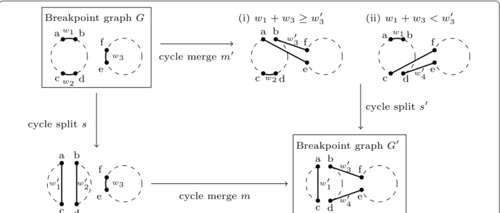
by s from C1 ; see Fig. 1 for an illustration. Now let
us consider m. Wlog, let us suppose that m acts on Cb and another cycle C2�= Ca (since df-sequences are
excluded), in order to produce cycle C3. It is easy to see
that if m cuts an edge different from bd in Cb, then s and
m are two independent wDCJ, and thus can be safely
swapped. Thus we now assume that m cuts bd. Suppose the edge that is cut in C2 is ef, of weight w3, and that
the joins are edges bf and de, of respective weights w′ 3
and w′
4. We thus have w′3+ w4′ = w2′ + w3 (b). Moreover,
adding (a) and (b) gives w1+ w2+ w3= w′1+ w′3+ w4′
(c). Now let us show that there exists a scenario that allows to obtain Ca and C3 from C1 and C2, which begins
by a merge followed by a split. For this, we consider two cases:
• w1+ w3≥ w3′ [see Fig. 1(i)]: m′ consists in cutting
ab from C1 and ef from C2, then forming ae and
bf, so as to obtain a unique cycle C. Note that C
now contains edges cd (of weight w2), bf (of weight
w′
3 ) and ae (of weight w1+ w3− w3′, which is non
negative by hypothesis). Then, s′ is defined as
follows: cut ae and cd, form edges ac, de. Finally, note that assigning w′
1 to ac and w′4 to de is possible,
since ae is of weight w1+ w3− w′3, cd is of weight
w2, and since w1+ w3− w3′ + w2= w′1+ w′4 by (c).
• w1+ w3<w′3 [see Fig. 1(ii)]. Consider the
fol-lowing merge m′: cut edges cd and ef, and form
the edges de of weight w′
4, and cf of weight
w = w2+ w3− w4′. This merge is feasible because
w ≥ 0: indeed, by hypothesis w1+ w3<w′3, i.e.
w1+ w2+ w3<w2+ w3′, which by (c) implies
w′
1+ w′4<w2. Thus w′4<w2, and consequently
w > w3≥ 0. Now let s′ be as follows: cut ab (of
weight w1) and cf (of weight w = w2+ w3− w′4 )
to form edges ac and bf of respective weights w′
1 and w′3. Note that s′ is always feasible since
w1+ w = w1+ w2+ w3− w′4= w′1+ w3′ by (c).
In all cases, it is always possible to obtain G′, starting
from G, using a merge m′ followed by a split s′, rather
than s followed by m, and the result is proved.
Fig. 1 Two different scenarios that lead to G′ starting from G: (downward) a split s followed by a merge m ; (rightward) a merge m′ followed by a split
Proposition 4 In an optimal wDCJ sorting scenario, no
cycle freeze or df-sequence occurs.
Proof Suppose a wDCJ sorting scenario contains at least
one cycle freeze or df-sequence, and let us consider the last such event f that appears in it. We will show that there also exists a sorting scenario that does not contain f, and whose length is decreased by at least one. For this, note that the sequence of wDCJ that follow f, say S, is only composed of cycle splits and merges which do not form df-sequences. By Proposition 3, in S any split that precedes a merge can be replaced by a merge that precedes a split, in such a way that the new scenario is a sorting one, and of same length. By iterating this process, we end up with a sequence S′ in
which, after f, we operate a series M of merges, followed by a series S of splits. Let GM be the breakpoint graph obtained
after all M merges are applied. If a cycle was unbalanced in GM, any split would leave at least one unbalanced cycle,
and it would be impossible to finish the sorting by apply-ing the splits in S. Thus GM must contain only balanced
cycles. Recall that f acts inside a given cycle C, while main-taining its imbalance I(C) unchanged. C may be iteratively merged with other cycles during M, but we know that, in GM , the cycle C′ that finally “contains” C is balanced. Thus,
if we remove f from the scenario, the breakpoint graph G′ M
we obtain only differs from GM by the fact that C′ is now
replaced by another cycle C′′, which contains the same
ver-tices and is balanced. However, by Proposition 2, we know that G′
M can be optimally sorted using the same number of
splits as GM, which allows us to conclude that there exists a
shorter sorting scenario that does not use f.
Proposition 5 Any wDCJ sorting scenario can be
trans-formed into another wDCJ sorting scenario of same or shorter length, and in which any cycle merge occurs before any cycle split.
Proof By Proposition 4, we can transform any sorting scenario into one of same or shorter length that contains no cycle freeze nor df-sequence. Moreover, by Propo-sition 3, if there exist two consecutive wDCJ which are respectively a cycle split and a cycle merge, they can be replaced by a cycle merge followed by a cycle split, lead-ing to a scenario that remains sortlead-ing and of same length. Thus, it is possible to iterate such an operation until no cycle split is directly followed by a cycle merge, i.e. all merges are performed before all splits.
Proposition 6 In an optimal wDCJ sorting scenario, no
balanced cycle is ever merged.
Proof We know that no optimal wDCJ scenario
con-tains a cycle freeze or a df-sequence (Proposition 4). We
also can assume that the scenario is such that all merges appear before all splits (Proposition 5). Let M (resp. S) be the sequence of merges (resp. splits) in this scenario. Let us suppose that at least one balanced cycle is merged in this scenario, and let us observe the last such merge
m. Among the two cycles that are merged during m,
at least one, say C1, is balanced. Let us call C1′ the cycle
that “contains” C1 after M is applied, and let GM be the
breakpoint graph obtained after M is applied. We know that GM only contains balanced cycles, as no split can
generate two balanced cycles from an unbalanced one. In particular, C′
1 is balanced. Let c denote the number
of cycles in GM. We know by Proposition 2 that it takes
exactly n − c wDCJ to sort GM, leading to a scenario of
length l = |M| + n − c. Now, if we remove m from M and look at the graph G′
M obtained after all merges are
applied, G′
M contains the same cycles as GM, except that
C′
1 is now “replaced” by two balanced cycles C1′′ and C1,
where the vertices of C′
1 are the same as the ones from C1′′
and C1. Thus, by Proposition 2, it takes exactly n − (c + 1)
wDCJ to sort G′
M, which leads to a scenario of length
l′= |M| − 1 + n − (c + 1) = l − 2 and contradicts the
optimality of the initial scenario. Hence m does not hap-pen in an optimal wDCJ sorting scenario, and the propo-sition is proved. Based on the above results, we are now able to derive a formula for the wDCJ distance, which is somewhat similar to the “classical” DCJ distance formula [5].
Theorem 7 Let BG(g1,g2) be the breakpoint graph of
two genomes g1 and g2, and let c be the number of cycles
in BG(g1,g2). Then wDCJ(g1,g2)= n − c + 2m, where m
is the minimum number of cycle merges needed to obtain a set of balanced cycles from the unbalanced cycles of
BG(g1,g2).
Proof By the previous study, we know that there exists
an optimal wDCJ scenario without cycle freezes or df-sequences, and in which merges occur before splits (Propositions 4, 5). We also know that before the splits start, the graph GM we obtain is a collection of balanced
cycles, and that the split sequence that follows is optimal and only creates balanced cycles (Proposition 2). Thus the optimal distance is obtained when the merges are as few as possible. By Proposition 6, we know that no balanced cycle is ever used in a cycle merge in an optimal scenario. Hence an optimal sequence of merges consists in creating balanced cycles from the unbalanced cycles of BG(g1,g2)
only, using a minimum number m of merges. Alto-gether, we have (i) m merges that lead to c − m cycles, then (ii) n − (c − m) splits by Proposition 2. Hence the
Algorithmic aspects of wDCJ‑dist
Based on the properties of a(n optimal) wDCJ sorting sce-nario given in “Main properties of sorting by wDCJ’’, we are now able to provide algorithmic results concerning the wDCJ-dist problem.
Complexity of wDCJ‑dist
The computational complexity of wDCJ-dist is given by the following theorem. As there are numerical values in the input of wDCJ-dist, the complexity has to be established in a weak or strong form, i.e. considering numbers in the input in binary or unary notation.
Theorem 8 The wDCJ-dist problem is strongly NP-
complete.
Proof The proof is by reduction from the strongly
NP-complete 3-Partition problem [11], whose instance is a multiset A = {a1,a2. . .a3n} of 3n positive integers
such that (i) 3n
i=1ai= B · n and (ii) B4 <ai< B2 for any
1 ≤ i ≤ 3n, and where the question is whether one can partition A into n multisets A1. . .An, such that for each
1 ≤ i ≤ n, aj∈Aiaj= B. Given any instance A of
3-Par-tition, we construct two genomes g1 and g2 as follows:
g1 and g2 are built on a vertex set V of cardinality 8n, and
consist of the same perfect matching. Thus BG(g1,g2)
is composed of 4n trivial cycles, that is cycles of length 2, say C1,C2. . .C4n. The only difference between g1 and g2
thus lies on the weights of their edges. For any 1 ≤ i ≤ 4n, let e1
i (resp. e 2
i) be the edge from Ci that belongs to g1
(resp. g2). The weight we give to each edge is the
follow-ing: for any 1 ≤ i ≤ 3n, w(e1
i)= ai and w(e 2
i)= 0; for any
3n + 1 ≤ i ≤ 4n, w(e1i)= 0 and w(ei2)= B. As a conse-quence, the imbalance of each cycle is I(Ci)= ai for any
1 ≤ i ≤ 3n, and I(Ci)= −B for any 3n + 1 ≤ i ≤ 4n. Now
we will prove the following equivalence: 3-Partition is satisfied iff wDCJ(g1,g2)≤ 6n.
(⇒) Suppose there exists a partition A1. . .An of A such
that for each 1 ≤ i ≤ n, aj∈Aiaj= B. For any 1 ≤ i ≤ n ,
let Ai = {ai1,ai2,ai3}. Then, for any 1 ≤ i ≤ n, we merge
cycles Ci1, Ci2 and Ci3, then apply a third merge with C3n+i.
For each 1 ≤ i ≤ n, these three merges lead to a bal-anced cycle, since after the two first merges, the obtained weight is ai1 + ai2 + ai3 = B. After these 3n merges (in
total) have been applied, we obtain n balanced cycles, from which 4n − n = 3n splits suffice to end the sorting, as stated by Proposition 2. Thus, altogether we have used 6n wDCJ, and consequently wDCJ(g1,g2)≤ 6n.
(⇐) Suppose that wDCJ(g1,g2)≤ 6n. Recall that in
the breakpoint graph BG(g1,g2), we have c = 4n cycles
and 8n vertices. Thus, by Theorem 7, we know that wDCJ (g1,g2)= 4n − 4n + 2m = 2m, where m is the
smallest number of merges that are necessary to obtain
a set of balanced cycles from BG(g1,g2). Since we
sup-pose wDCJ(g1,g2)≤ 6n, we conclude that m ≤ 3n.
Oth-erwise stated, the number of balanced cycles we obtain after the merges cannot be less than n, because we start with 4n cycles and apply at most 3n merges. However, at least four cycles from C1,C2. . .C4n must be merged
in order to obtain a single balanced cycle: at least three from C1,C2. . .C3n (since any ai satisfies B4 <ai< B2 by
definition), and at least one from C3n+1,C3n+2. . .C4n (in
order to end up with an imbalance equal to zero). Thus any balanced cycle is obtained using exactly four cycles (and thus three merges), which in turn implies that there exists a way to partition the multiset A into A1. . .An
in such a way that for any 1 ≤ i ≤ n, ( aj∈Ai)− B = 0,
which positively answers the 3-Partition problem.
Approximating wDCJ‑dist
Since wDCJ-dist is NP-complete, we now look for algo-rithms that approximately compute the wDCJ distance. We first begin by the following discussion: let g1 and g2 be
two evenly weighted genomes, where Cu= {C1,C2. . .Cnu}
is the set of unbalanced cycles in BG(g1,g2). It can be seen
that any optimal solution for wDCJ-dist will be obtained by merging a maximum number of pairs of cycles {Ci,Cj}
from Cu such that I(Ci)+ I(Cj)= 0, because each such pair
represents two unbalanced cycles that become balanced when merged. Let S2= {Ci1,Ci2. . .Cin2} be a maximum
cardinality subset of Cu such that I(Cij)+ I(Cij+1)= 0 for
any odd j, 1 ≤ j < n2: S2 thus contains a maximum
num-ber of cycles that become balanced when merged by pairs. Note that S2 can be easily computed by a greedy algorithm
that iteratively searches for a number and its opposite among the imbalances in Cu. Now, C′u= Cu\ S2 needs to
be considered. It would be tempting to go one step further by trying to extract from C′u a maximum number of triplets
of cycles whose imbalances sum to zero. This leads us to define the following problem:
Max‑Zero‑Sum‑Triplets (MZS3)
Instance: A multiset P = {p1,p2. . .pn} of numbers
pi∈ Z∗ such that for any 1 ≤ i, j ≤ n, pi+ pj�= 0.
Output: A maximum cardinality set P′ of non
intersect-ing triplets from P, such that each sums to zero.
Note that the multiset P in the definition of MZS3 cor-responds to the multiset of imbalances of C′u in
wDCJ-dist. The next two propositions (Propositions 9, 10) consider resp. the computational complexity and approx-imability of MZS3. The latter will be helpful for devising an approximation algorithm for wDCJ-dist, as shown in Theorem 11 below.
Proposition 9 The MZS3 problem is strongly NP-
Proof The proof is by reduction from Numerical
3-Dimensional Matching (or N3DM), a decision prob-lem defined as follows: given three multisets of posi-tive integers W, X and Y containing m elements each, and a positive integer b, does there exist a set of triplets T ⊆ W × X × Y in which every integer from W, X, Y appears in exactly one triplet from T, and such that for every triplet {w, x, y} ∈ T, w + x + y = b? The N3DM problem has been proved to be strongly NP-complete in [11]. Note that, in addition, we can always assume that any element s in W, X or Y satisfies s < b, otherwise the answer to N3DM is clearly negative.
Given a set S of integers and an integer p, we denote by S + p (resp. S − p) the set containing all ele-ments of S to which p has been added (resp. sub-tracted). Given any instance I = {W , X, Y , b} of N3DM, we construct the following instance of MZS3: I′= P = (W + b) ∪ (X + 3b) ∪ (Y − 5b). Note that P
contains n = 3m elements that all strictly lie between −5b and 4b ; thus the input size of I′ does not exceed a
constant times the input size of I. Note also that no two elements s, t ∈ P are such that s + t = 0, because each negative (resp. positive) element in P is strictly less than −4b (resp. than 4b).
We now claim that the answer to N3DM on I is positive iff MZS3 outputs exactly m =n
3 independent triplets,
each summing to zero.
(⇒) Suppose the answer to N3DM on I is positive, and let
T be the output set. The answer to MZS3 is constructed as
follows: for any triplet {w, x, y} that sums to zero in T, add {w + b, x + 3b, y − 5b} to P′. Since T covers all elements
from W, X and Y exactly once, then P′ contains exactly
m =n3 non intersecting triplets. Besides, each triplet sums
to (w + b) + (x + 3b) + (y − 5b) = (x + y + w) − b = 0 since x + y + w = b by assumption.
(⇐) Suppose there exist n
3 non intersecting triplets
{fi,gi,hi} in P, 1 ≤ i ≤ n3 such that fi+ gi+ hi= 0. Our
goal is to show that (wlog) fi∈ W + b, gi ∈ X + 3b and
hi∈ Y − 5b. As mentioned above, we can assume that
any element in W, X, Y strictly lies between 0 and b. Thus we have the following set of inequalities:
• any element w ∈ (W + b) satisfies b < w < 2b • any element x ∈ (X + 3b) satisfies 3b < x < 4b • any element y ∈ (Y − 5b) satisfies −5b < y < −4b It can be seen from the above inequalities that any tri-plet that sums to zero must take one value in each of the sets (W + b), (X + 3b) and (Y − 5b) (otherwise the sum is either strictly negative or strictly positive). Thus, for each {fi,gi,hi} returned by MZS3, we add
{fi′,gi′,h′i} = {(fi− b), (gi− 3b), (hi+ 5b)} to T. We now
claim that T is a positive solution to N3DM: each triplet
{fi′,gi′,h′i} is taken from W × X × Y , T covers each
ele-ment of W, X and Y exactly once, and for any 1 ≤ i ≤ n 3 ,
f′
i + gi′+ h′i= b since fi+ gi+ hi= 0.
Proposition 10 The MZS3 problem is 1
3-approximable.
Proof The approximation algorithm we provide here is a
simple greedy algorithm we will call A, which repeats the following computation until P is empty: for each num-ber x in P, find two numnum-bers y and z in P \ {x} such that y + z = −x. If such numbers exist, add triplet {x, y, z} to the output set P′ and remove x, y and z from P; otherwise
remove x from P. We claim that A approximates MZS3 within a ratio of 1
3. For this, consider an optimal
solu-tion, say Opt={t1,t2. . .tm} consisting of m independent
triplets from P such that each sums to zero, and let us compare it to a solution Sol = {s1,s2. . .sk} returned by
A. First, note that any ti, 1 ≤ i ≤ m necessarily intersects
with an sj, 1 ≤ j ≤ m, otherwise ti would have been found
by A, a contradiction. Moreover, any element of a triplet ti from Opt is present in at most one triplet from Sol.
Now, it is easy to see that necessarily m ≤ 3k, since for any 1 ≤ i ≤ m, the three elements of a ti intersect with at
least one and at most three different sjs. Thus A achieves
the sought approximation ratio of 1
3.
Theorem 11 The w problem is DCJ-dist4
3-approximable.
Proof Our approximation algorithm A′ considers the
set Cu of unbalanced cycles and does the following:
(a) find a maximum number of pairs of cycles whose imbalances sum to zero, and merge them by pairs, (b) among the remaining unbalanced cycles, find a max-imum number of triplets of cycles whose imbalances sum to zero and merge them three by three, (c) merge the remaining unbalanced cycles into a unique (bal-anced) cycle. Once this is done, all cycles are balanced, and we know there exists an optimal way to obtain n balanced trivial cycles from this point (see Proposi-tion 2). We note n2 (resp. n3) the number of cycles
involved in the pairs (resp. triplets) of (a) [resp. (b)]. As previously discussed, n2 can easily be computed, and
n3 is obtained by solving MZS3. We know that MZS3
is NP-complete (Proposition 9), and more importantly that MZS3 is 1
3-approximable (Proposition 10) ; in other
words, step (b) of algorithm A′ finds n′
3≥ n33 (otherwise
stated, n′
3= n33 + x with x ≥ 0 ) cycles that become
bal-anced when merged by triplets. We will show in the rest of the proof that A′ approximates wDCJ(g1,g2) within
ratio 4 3.
First let us estimate the number mA′ of
mA′ = n22 +2n93 + 23x + (nu− n2− (n33 + x) − 1) , and
that after these merges have been done, we are left with c′= n
b+n22 + n3
9 +x3+ 1 balanced cycles.
Thus, by Proposition 2, the number of splits sA′
that follow satisfies sA′ = n − c′, and the total
num-ber of wDCJ operated by A′, say dcjA′, satisfies
dcjA′ = mA′+ sA′ = n − nb+ n93 + x3+ (nu− n2− n3
3
−x − 2) . In other words, since x ≥ 0, we have that dcjA′ ≤ n − nb+ nu− n2−2n93 [inequality (I1)]. Now
let us observe an optimal sorting scenario of length wDCJ (g1,g2), which, as we know by the results in “Main
properties of sorting by wDCJ’’, can be assumed to
con-tain mopt merges followed by sopt splits. In any optimal
scenario, the best case is when all of the n2 cycles are
merged by pairs, all of the n3 cycles are merged by
tri-plets, and the rest is merged four by four, which leads to mopt≥ n22 +
2n3
3 +
3(nu−n2−n3)
4 . In that case, we obtain
c′
opt≤ nb+ n22 + n3
3 +
nu−n2−n3
4 balanced cycles,
lead-ing to sopt = n − copt′ ≥ n − nb−n22 − n3
3 −
nu−n2−n3 4
subsequent splits. Altogether, we conclude that wDCJ (g1,g2)= mopt+ sopt ≥ n − nb+n33 +
nu−n2−n3
2 ,
that is wDCJ(g1,g2)≥ n − nb+n2u − n22 − n63
[inequality (I2)].
Our goal is now to show that dcjA′ ≤ 43· wDCJ (g1,g2) .
For this, it suffices to show that 4 · wDCJ(g1, g2)
−3 · dcjA′ ≥ 0. Because of inequalities (I1) and (I2)
above, 4 · wDCJ(g1,g2)− 3 · dcjA′ ≥ 0 is satisfied whenever S ≥ 0, where S = 4 · (n − nb+ nu 2 − n2 2 − n3 6) −3 · (n − nb+ nu− n2− 2n3
9 ). It can be easily seen
that S = n − nb− nu+ n2. Note that we always have
n ≥ nb+ nu since n is the maximum possible number of
cycles in BG(g1,g2) ; besides, n2≥ 0 by definition. Thus
we conclude that S ≥ 0, which in turn guarantees that our algorithm A′ approximates wDCJ-dist within the sought
ratio of 4
3.
FPT issues concerning wDCJ‑dist
Recall first that by Theorem 7, for any genomes g1 and
g2 , wDCJ(g1,g2)= n − c + 2m, where m is the minimum
number of cycle merges needed to obtain a set of balanced cycles from the unbalanced cycles of BG(g1,g2) .
The NP-completeness of wDCJ-dist thus comes from the fact that computing m is hard, since n and c can be computed polynomially from g1 and g2. Computing m is
actually closely related to the following problem:
Max‑Zero‑Sum‑Partition (MZSP)
Instance: A multiset S = {s1,s2. . .sn} of numbers si∈ Z∗
s.t. n
i=1si = 0.
Output: A maximum cardinality partition {S1,S2. . .Sp}
of S such that sj∈Sisj= 0 for every 1 ≤ i ≤ p.
Indeed, let Cu = {C1,C2. . .Cnu} be the set of
unbalanced cycles in BG(g1,g2). If S represents the
multiset of imbalances of cycles in Cu, then the
parti-tion {S1,S2. . .Sp} of S returned by MZSP implies that
for every 1 ≤ i ≤ p, |Si| − 1 cycles merges will be
oper-ated in order to end up with p balanced cycles. Thus, a total of p
i=1(|Si| − 1) = nu− p merges will be used.
In other words, the minimum number of cycle merges m in the expression wDCJ(g1,g2)= n − c + 2m satisfies
m = nu− p, where p is the number of subsets of S returned
by MZSP. Note that MZSP is clearly NP-hard, since other-wise we could compute wDCJ(g1,g2)= n − c + 2(nu− p)
in polynomial-time, a contradiction to Theorem 8.
A classical parameter to consider when studying FPT issues for a given minimization problem is the “size of the solution”. In our case, it is thus legitimate to ask whether wDCJ-dist is FPT in wDCJ(g1,g2). However, it can be
seen that wDCJ(g1,g2)≥ m since n − c is always positive,
and that m ≥ nu
2 since all cycles in Cu are unbalanced
and it takes at least two unbalanced cycles (thus at least one merge) to create a balanced one. Thus, proving that wDCJ-dist is FPT in nu, as done in Theorem 12 below,
comes as a stronger result.
Theorem 12 The wDCJ-dist problem can be solved in
O∗(3nu), where n
u is the number of unbalanced cycles in
BG(g1,g2).
Proof By Theorem 7 and the above discussion, it suf-fices to show that MZSP is FPT in n = |S|, and more precisely can be solved in O∗(3n), to conclude. Indeed,
if this is the case, then replacing S by the multiset of imbalances of cycles in Cu in MZSP (thus with n = nu)
allows us to compute m, and thus wDCJ(g1,g2), in time
O∗(3nu). Note first that MZSP is clearly FPT in n, just by
brute-force generating all possible partitions of S, testing whether it is a valid solution for MZSP, and keeping one of maximum cardinality among these. The fact that the complexity of the problem can be reduced to O∗(3n) is
by adapting the Held-Karp Dynamic Programming algo-rithm [12, 13], which we briefly describe here. The main idea is to fill a dynamic programming table D(T, U), for any non-intersecting subsets T and U of S, where D(T, U) is defined as the maximum number of subsets summing to zero in a partition of T ∪ U, with the additional con-straint that all elements of T belong to the same subset. The number p that corresponds to a solution of MZSP is thus given by D(∅, S). For any nonempty subset X ⊆ S, we let s(X) = si∈Xsi. Table D is initialized as follows:
D(∅, ∅) = 0, D(T, ∅) = −∞ for any T �= ∅ such that s(T ) �= 0, and D(T, U) = 1 + D(∅, U) for any T �= ∅ such that s(T) = 0. Finally, the main rule for filling D is
D(T , U ) = max
It can be seen that computing any entry in table D is achievable in polynomial time, and that the number of entries is 3n. Indeed, any given element of S appears
either in T, in U, or in S \ (T ∪ U): this can be seen as a partition of S into three subsets, and 3n such partitions
exist. Altogether, we have that p is computable in O∗(3n)
– and this is also the case for the corresponding partition {S1,S2. . .Sp} of S, that can be retrieved by a backward
search in D.
An integer linear programming for solving wDCJ‑dist
The ILP we propose here actually consists in solving the MZSP problem. Once this is done, the number p of sets in the output partition is easily retrieved, as well as wDCJ (g1,g2) since wDCJ(g1,g2)= n − c + 2(nu− p), as
discussed before Theorem 12. We also recall that p ≤nu 2 ,
since it takes at least two unbalanced cycles to create a balanced one.
Our ILP formulation is given in Fig. 2 and described hereafter: we first define binary variables xi,j, for
1 ≤ i ≤ nu and 1 ≤ j ≤ n2u, that will be set to 1 if the
unbalanced cycle Ci ∈ Cu belongs to subset Cj, and
0 otherwise. The binary variables pi, 1 ≤ i ≤ n2u, will
simply indicate whether Ci is “used” in the solution, i.e
pi= 1 if Ci�= ∅, and 0 otherwise. In our ILP formulation,
(2) ensures that each unbalanced cycle is assigned to exactly one subset Ci; (3) requires that the sum of the
imbalances of the cycles from Ci is equal to zero. Finally,
(4) ensures that a subset Ci is marked as unused if no
unbalanced cycle has been assigned to it. Moreover, since the objective is to maximize the number of non-empty subsets, pi will necessarily be set to 1 whenever Ci�= ∅.
Note that the size of the above ILP depends only on nu, as
it contains �(n2
u) variables and �(nu) constraints.
A probabilistic model of evolution by wDCJ
In this section, we define a model of evolution by wDCJ, in order to derive theoretical and empirical bounds for the parameter nu on which both the FPT and ILP
algo-rithms depend. The model is a Markov chain on all
weighted genomes (that is, all weighted perfect match-ings) on 2n vertices. Transitions are wDCJ, such that from one state, two distinct edges ab and cd are chosen uniformly at random, and replaced by either ac and bd or by ad and cb (with probability 0.5 each). Weights of the new edges are computed by drawing two numbers
x and y uniformly at random in respectively [0, w(ab)]
and [0, w(cd)], and assigning x + y to one edge, and w(ab) + w(cd) − x − y to the other (with probability 0.5 each).
Proposition 13 The equilibrium distribution of this
Markov chain is such that a genome has a probability proportional to the product of the weights on its edges. Proof Define as the probability distribution over the space of all genomes, such that for a genome g, �(g) is proportional to �e∈E(g)w(e). Let P(g1,g2) be the
transi-tion probability in the Markov chain between weighted genomes g1 and g2. We have that P(g1,g2)= 0 unless
g1 and g2 differ only by two edges, say ab and cd in
g1 and ac and bd in g2. In that case, suppose wlog that
w(ab) < w(cd) and that w(ac) = x + y, where x and y are the numbers drawn by the model. We have two cases. If w(ac) < w(ab), then P(g1,g2)∼ w(ac)/(w(ab)w(cd))
because there are exactly w(ac) combinations of x and
y which can transform g1 into g2, over a total
num-ber of possibilities (w(ab)w(cd)); by the same reason-ing, P(g2,g1)∼ 1/w(cd), and if w(ac) > w(ab), then
P(g1,g2)∼ 1/w(bd) and P(g2,g1)∼ w(ab)/(w(ac)w(bd)) .
In all cases, �(g1)P(g1,g2)= �(g2)P(g2,g1), hence is
the equilibrium distribution of the Markov chain. As a consequence, the weight distributions follow a symmetric Dirichlet law with parameter α = 2. It is possible to draw a genome at random in the equilibrium distribution by drawing a perfect matching uniformly at random and distributing its weights with a Gamma law of parameters 1 and 2.
We first prove a theoretical bound on the number of expected unbalanced cycles, and then show by simula-tions that this number probably stays far under this theo-retical bound on evolutionary experiments.
Theorem 14 Given a weighted genome g1 with nedges,
if k random wDCJ are applied tog1 to give a weighted
genome g2, then the expected number of unbalanced cycles
in BG(g1,g2) satisfies E(nu)= O(k/√n).
Proof In this proof, for simplicity, let us redefine the size of a cycle as half the number of its edges. Let n+
u (resp. n−u )
be the number of unbalanced cycles of size greater than or equal to (resp. strictly less than) √n. We thus have
nu= n+u + n−u. We will prove that (i) n+u ≤ k/ √ n and (ii) E(n− u)= O(k/ √ n).
First, if the breakpoint graph contains u unbalanced cycles of size at least s, then the number k of wDCJ is at least us. Indeed, by Theorem 7 the wDCJ distance is at least n − c + u, and as n ≥ us + (c − u), we have k ≥ us + (c − u) − c + u = us. As a consequence, k ≥ n+
u ·
√
n, and (i) is proved.
Second, any unbalanced cycle of size strictly less than s is the product of a cycle split. Given a cycle C of size r > s with r �= 2s, there are r possible wDCJ which can split C and produce one cycle of size s. If r = 2s, there are r / 2 possible splits which result in 2 cycles of size s. So there are O(sr) ways of splitting C and obtaining an unbal-anced cycle of size less than s. If we sum over all cycles, this makes O(sn) ways because the sum of the sizes of all cycles is bounded by n. As there are O(n2) possible wDCJ
in total, the probability to split a cycle of size r and obtain an unbalanced cycle of size less than s at a certain point of a scenario is O(s/n). If we sum over all the scenarios of
k wDCJ, this makes an expected number of unbalanced
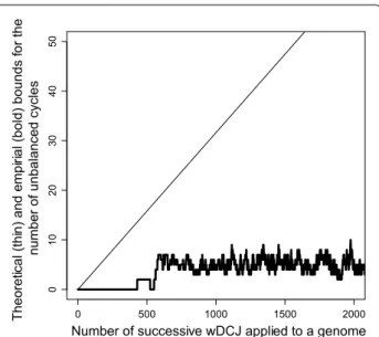
cycles in O(ks/n), which implies (ii) since s <√n. We simulated a genome evolution with n = 1000, and the weights on a genome drawn from the above discussed equilibrium distribution. Then we applied k=10,000 wDCJ, and we measured the value of nu on the way. As
shown in Fig. 3 (up to k = 2000 for readability), nu does
not asymptotically grow with k (in the whole simulation a
maximum of 13 was reached for k around 5500, while the mean does not grow up to k=10,000). This tends to show that the theoretical bound given in Theorem 14 is far from being reached in reality, and that parameter nu is very low
is this model. We actually conjecture that the expected number E(nu)= o(n) and in particular does not depend
on k. Nevertheless, this shows that, in practice, both the FPT and ILP algorithms from the previous section should run in reasonable time on this type of instances. As an illustration, we ran the ILP algorithm described in Fig. 2
on a set of 10,000 instances generated as described above. For each of these instances, the execution time on a stand-ard computer never exceeded 8 ms.
As a side remark, we note that the model presented here is different from the one used in Biller et al. [3], in which rearrangements are drawn with a probability pro-portional to the product of the weights of the involved edges. We checked that the behavior concerning nu was
the same in both models ; however, we were unable to adapt proof of Theorem 14 to that case.
Conclusion and perspectives
We made a few steps in the combinatorial study of rear-rangement operations which depend on and affect inter-gene sizes. We leave open many problems and extensions based on this study. First, we would like to raise the two following algorithmic questions: is wDCJ-dist APX-hard? Can we improve the O∗(3nu) time complexity to
solve wDCJ-dist? Second, the applicability of our model to biological data lacks additional flexibility, thus we sug-gest two (non exclusive) possible extensions: (a) give a weight to every wDCJ, e.g. a function of the weights of the involved edges; (b) instead of assuming that the total intergene size is conservative (which is not the case in biological data), consider a model in which intergene size may be altered by deletions, insertions and duplica-tions—note that such a study is initiated in [9]. Third, generalizing the model to non co-tailed genomes (in our terminology, matchings that are not perfect) remains an open problem. It is clearly NP-complete, as it general-izes our model, but other algorithmic questions, such as approximability and fixed-parameter tractability, remain to be answered. Statistical problems are also numer-ous in this field. A first obvinumer-ous question would be to improve the bound of Theorem 14, as it seems far from being tight when compared to simulations. Finally, we note that the present study compares two genomes with equal gene content, whereas realistic situations concern an arbitrary number of genomes with unequal gene con-tent. This calls for extending the present work to more general models.
Authors’ contributions
All authors read and approved the final manuscript.
0 500 1000 1500 2000 01 02 0 30 40 50
Number of successive wDCJ applied to a genome
Theoret
ic
al (thi
n) and empi
rial (bold) bounds
fo
r the
number of unbalanced cycles
Fig. 3 Number of unbalanced cycles (y axis), in a simulation on
genomes with n = 1000 edges where k wDCJ operations are applied successively (k is on the x axis). The number of unbalanced cycles is computed (i) according to the theoretical bound k/√n (in thin), and (ii) directly from the simulated genomes (in bold)
• We accept pre-submission inquiries
• Our selector tool helps you to find the most relevant journal
• We provide round the clock customer support
• Convenient online submission
• Thorough peer review
• Inclusion in PubMed and all major indexing services
• Maximum visibility for your research Submit your manuscript at
www.biomedcentral.com/submit
Submit your next manuscript to BioMed Central
and we will help you at every step:
Author details
1 LS2N UMR CNRS 6004, Université de Nantes, 2 rue de la Houssinière, 44322 Nantes, France. 2 Institut National de Recherche en Informatique et en Automatique (Inria) Grenoble Rhône-Alpes, 655 avenue de l’Europe, 38330 Montbonnot-Saint-Martin, France. 3 CNRS, Laboratoire de Biomètrie et Biologie Evolutive UMR5558, Univ Lyon, Université Lyon 1, 43 boulevard du 11 novembre 1918, 69622 Villeurbanne, Villeurbanne, France.
Acknowledgements
The authors would like to thank Tom van der Zanden from U. Utrecht (Netherlands) for the rich discussions we had concerning the MZSP problem.
Supported by GRIOTE project, funded by Région Pays de la Loire, and the ANCESTROME project, Investissement d’avenir ANR-10-BINF-01-01.
A preliminary version of this paper appeared in Proceedings of the 16th Workshop on Algorithms in Bioinformatics (WABI 2016) [10].
Competing interests
The authors declare that they have no competing interests.
Publisher’s Note
Springer Nature remains neutral with regard to jurisdictional claims in published maps and institutional affiliations.
Received: 5 January 2017 Accepted: 15 May 2017
References
1. Fertin G, Labarre A, Rusu I, Tannier E, Vialette S. Combinatorics of genome rearrangements. Computational molecular biology. Cambridge: MIT Press; 2009. p. 312.
2. Lynch M. The Origin of Genome Architecture. Sunderland, USA: Sinauer; 2007.
3. Biller P, Guéguen L, Knibbe C, Tannier E. Breaking good: accounting for the diversity of fragile regions for estimating rearrangement distances. Genome Biol Evol. 2016;8:1427–39.
4. Biller P, Knibbe C, Beslon G, Tannier E. Comparative genomics on artificial life. In: Beckmann A, Bienvenu L, Jonoska N, editors. Proceedings of Pursuit of the Universal-12th conference on computability in Europe, CiE 2016, Lecture notes in computer science, vol. 9709, Paris, France, June 27–July 1, 2016. Berlin: Springer; 2016. p. 35–44.
5. Yancopoulos S, Attie O, Friedberg R. Efficient sorting of genomic permu-tations by translocation, inversion and block interchange. Bioinformatics. 2005;21(16):3340–6.
6. Baudet C, Dias U, Dias Z. Length and symmetry on the sorting by weighted inversions problem. In: Campos SVA, editor. Advances in bioinformatics and computational biology - 9th Brazilian symposium on bioinformatics, BSB 2014, Belo Horizonte, October 28–30, 2014, Proceed-ings, vol. 8826., Lecture notes in computer scienceBerlin: Springer; 2014. p. 99–106.
7. Swenson KM, Blanchette M. Models and algorithms for genome rear-rangement with positional constraints. In: Pop M, Touzet H, editors. Algorithms in bioinformatics-15th international workshop, WABI 2015, Atlanta,September 10–12, 2015, Proceedings, vol. 9289., Lecture notes in computer scienceBerlin: Springer; 2015. p. 243–56.
8. Alexeev N, Alekseyev MA. Estimation of the true evolutionary distance under the fragile breakage model. In: IEEE 5th international conference on computational advances in Bio and medical sciences; 2015 9. Bulteau L, Fertin G, Tannier E. Genome rearrangements with
indels in intergenes restrict the scenario space. BMC Bioinform. 2016;17(S–14):225–31.
10. Fertin G, Jean G, Tannier E. Genome rearrangements on both gene order and intergenic regions. In: Frith MC, Pedersen CNS, editors. Proceedings lecture notes in computer science algorithms in bioinformatics-16th international workshop, WABI 2016, Aarhus, Denmark, August 22–24, 2016 , vol. 9838. Berlin: Springer; 2016. p. 162–173
11. Garey MR, Johnson DS. Computers and intractability; a guide to the theory of NP-completeness. New York: W. H. Freeman & Co; 1990. 12. Held M, Karp RM. A dynamic programming approach to sequencing
problems. J Soc Ind Appl Math. 1962;10(1):196–210. 13. van der Zanden T. Personal communication. 2016