Analysis of online algorithms for resource allocation applied to the stock market

Analysis of Online Algorithm for Resource Allocation

Applied to the Stock Market

by

Alexander Michael St. Clair Duran

Submitted to the Department of Electrical Engineering and Computer Science

in partial fulfillment of the requirements for the degrees of

Master of Engineering in Electrical Engineering and Computer Science

and

Bachelor of Science in Computer Science and Engineering

at the

MASSACHUSETTS INSTITUTE OF TECHNOLOGY

February 1999

@Alexander Michael St. Clair Duran, MCMXCIX. All rights reserved.

The author hereby grants to MIT permission to reproduce and distribute publicly

paper and electronic copies of this thesis document in whole or in part, and to grant

others the right to do so.

Z4 / I

A uthor ... ... ... -.-. . ...

Department of Electrical Engineering and Computer Science

February 9, 1999

Certified by

Tom Leighton

Professor of Applied Mathematics

Thesis Supervisor

) 2

Accepted by ...

..

Chairman, Department Committee

L ETTS INSTITUTE ECHNOLOGY

.... ... .. ... .... .. ..

Arthur C. Smith

on Graduate Theses

,,t/

,I /

Analysis of Online Algorithm for Resource Allocation Applied to the

Stock Market

by

Alexander Michael St. Clair Duran

Submitted to the Department of Electrical Engineering and Computer Science on February 9, 1999, in partial fulfillment of the

requirements for the degrees of

Master of Engineering in Electrical Engineering and Computer Science and

Bachelor of Science in Computer Science and Engineering

Abstract

In this thesis, I modified and implemented an algorithm which attempts to find and predict areas of good performance in a larger system where performance is random or adversarial. The algorithm was modified to work on a real stock market problem instead of an abstract problem. To test the algorithm, closing prices for every stock in the current S&P 500 were used, dating back to January 2, 1990.

Thesis Supervisor: Tom Leighton

Acknowledgments

I would first like to thank my thesis advisor Prof. Tom Leighton for helping me out with

this thesis. Without him, this thesis wouldn't have been written. Besides providing the

algorithm without which there would be no thesis to write, he helped me deal with prob-lems that arose during the course of this research. I would also like to thank my parents,

brothers, and friends who provided me with much needed moral support. Their words of encouragement and friendly derisive chiding helped me to get this done. To some of my friends I owe special thanks. Without them this thesis would have been even later and

con-siderably more over budget. My thanks go to Charles Hope, Jennifer Cunningham, Rebecca Merz, and Geoff Reber for proofreading and offering me helpful suggestions. Without them

I don't know what I would have done. Finally, I want to thank the teachers and staff of Course VI and the Institute in general. I really enjoyed my time here and they made that enjoyment possible.

Contents

1 Introduction

1.1 Options . . . .

1.1.1 The Black-Scholes Model

1.2 Technical Analysis . . . .

2 The New Algorithm

2.1 Abstract Stock Problem 2.2 The Algorithm . . . . .

3 Modification to Reality 3.1 Failure of the Model

3.1.1 Price Changes

3.1.2 Losing Money.

3.1.3 Investment After 3.1.4 Affecting Prices .

3.2 Storing the Money . . .

4 Results 4.1 Available Data . . . . . 4.2 Unrealistic Assumptions 4.3 Variance . . . . 4.4 Control Group . . . . . 4.5 Alternate Investment . . 4.6 Measuring Performance 4.7 Calculating D . . . . the Sale 8 8 10 11 12 . . . . 12 . . . . 13 16 . . . . 16 . . . . 17 . . . . 19 . . . . 19 . . . . 19 . . . . 20 21 21 22 23 24 24 25 26

4.8 Ways in Which the Algorithm was Run ... ... 26

4.9 Price Increases . . . . 27

4.9.1 The Continuous Model . . . . 27

4.9.2 The Once-a-day Model . . . . 32

4.10 Price D ecreases . . . . 35

4.10.1 The Continuous Model . . . . 35

4.10.2 The Once-a-day Model . . . . 40

4.11 Tests on New Data . . . . 42

5 Conclusions and Extensions 45 5.1 Conclusions . . . . 45

5.2 Suggestions for Further Research . . . . 46

A Main Program 47

B Data Preparing Program 64

C Result Compilation Program 70

D Result Calculation Program 1 75

E Result Calculation Program 2 (Alternate Investments) 80

List of Figures

4-1 Expected return on a single investment under the continuous transaction assumption when D was known and the goal was to make money . . . . 30

4-2 Expected return on algorithm stock selection minus expected return on ran-dom stock selection under the continuous model when D was known and the

goal was to make money . . . . 32

4-3 Expected return on a single investment under the once-a-day transaction assumption when D was known and the goal was to make money . . . . 33

4-4 Expected return on a single investment under the continuous transaction

assumption when D was known and the goal was to lose money . . . . 37

4-5 Expected return on algorithm stock selection minus expected return on ran-dom stock selection under the continuous model when D was known and the

goal was to lose money . . . . 38

4-6 Expected return on a single investment under the once-a-day transaction assumption when D was known and the goal was to lose money . . . . 42

List of Tables

2.1 An example of the abstract stock problem . . . . 13

2.2 Another example of the abstract stock problem. The adversary defeats a determ inistic strategy. . . . . 14

2.3 A third example of the abstract stock problem. The adversary competes

against a random strategy. . . . . 14

4.1 Results of attempting to make money under the continuous transaction as-sum ption . . . . 29

4.2 Results of attempting to make money under the continuous assumption and random stock selection . . . . 31

4.3 Results of attempting to make money under the once-a-day transaction as-sum ption . . . . 34 4.4 Results of attempting to lose money under the continuous transaction

as-sum ption . . . . 36

4.5 Results of attempting to lose money under the continuous assumption and random stock selection . . . . 39

4.6 Results of attempting to lose money under the once-a-day transaction as-sum ption . . . . 41 4.7 Results of running the algorithm on previously untested data starting

Chapter 1

Introduction

The problem of finding a way to reliably make money in the stock market is one that many people have attempted to solve. Stockbrokers and portfolio managers who have good track

records are in high demand. A computer algorithm that is successful at picking stocks would be a very useful asset to any investor. Unfortunately, since the stock market often seems to act much like a random walk, developing such an algorithm is not an easy task.

This paper analyzes one attempt at such an algorithm.

Chapter one describes some of the previous solutions to stock market prediction. Chap-ter two describes an abstract model of the stock market and a proposed algorithm for

making effective choices on when to buy and sell stocks. Chapter three describes the mod-ification of the real stock problem to sufficiently resemble the abstract problem so that the algorithm can be applied. Chapter four describes the results of experimentation. Chapter five discusses the conclusions to be drawn from the experiments and offers suggestions for

further applications of the algorithm to the stock problem.

Investors in the past have tried numerous approaches to developing a formula for stock

prediction. Unfortunately, a reliable and effective system for predicting price changes has thus far not been developed. Some methods have been developed, with mixed results. Two

of these methods are options pricing and technical analysis.

1.1

Options

One way in which investors attempt to profit from correctly predicting changes in stock prices is through buying and selling options. Options guarantee the buyer either a fixed

price at which the stock can be bought or a fixed price at which the stock can be sold. There are two types of options: call options and put options.

The writer of a call option guarantees to the buyer that on the expiration date of the

option, the stock for which the option was written can be bought by the buyer at the strike price of the option. The strike price is set when the option is first written, and generally matches the price of the stock at the time of writing. If, on the expiration date of the

option, the market price of the stock is higher than the strike price on the option, the buyer can make money by buying the stock at the strike price and then selling it at the market price. In practice, the option buyer just sells the option back and doesn't bother to actually

exercise it. If the market price is below the strike price, however, the option is worthless. The writer of the option makes a prediction that, on the date that the option expires, the market price of the stock will be less than the strike price of the option plus the option price, or premium. If the market price is lower than the strike price, the writer keeps the

entire premium. If the market price is between the strike price and the strike price plus premium, then the buyer can recoup some of the premium by selling the option, but the writer still makes a profit. If the market price is higher than the strike price plus premium, then the buyer gets more from selling the option than he spent on the premium, and the

writer loses money when forced to sell the stock to the buyer for significantly less than the market value of the stock.

A put option is the opposite of a call option. The writer of a put option guarantees

that the stock can be sold for the strike price. If the market price at the expiration date is lower than the strike price, then the buyer can buy the stock at the market price and then

exercise the option by selling the stock at the strike price. Again, in practice, the option is sold instead of being exercised. The writer of the option predicts that the market price will

be higher than the strike price. If his prediction is correct, or nearly so, he keeps some or all of the premium.

As a writer or buyer of options, it is important to know the fair value of the option. The fair value of an option is the value at which both the writer and the buyer are neutral about

trading the option. This value can, in theory, be computed by taking the expected return of the option for the buyer and subtracting a small amount for risk adjustment. For example, suppose that the buyer already has an option on stock A. The expected sale value of that

to compensate for the risk inherent in options, the fair value of the option is x - y. If this

were the premium, the buyer would be neutral about buying the option[3, pp. 165-168]. The main problem in determining the fair value of an option lies in calculating the

expected return. Calculating the expected return is similar to predicting what the stock price will do. It is not quite as specific, as it involves defining a probability function for the

stock price, whereas specific prediction attempts to nail down exactly what the price will do, but it still requires guessing (or knowing) what the stock price is likely to do. Therefore, options pricing is tied to the problem of predicting stock prices.

1.1.1 The Black-Scholes Model

A commonly used technique for calculating the fair value of an option is the Black-Scholes

model, developed by Fischer Black and Myron Scholes[3, pp. 195-199]. The Black-Scholes model simplifies the problem of determining fair option value, but makes some assumptions that adversely affect the accuracy of the model. These assumptions attempt to quantify how

stock prices behave. If the stock market doesn't behave in this manner, then the validity of the model is thrown into question. Three of the more important assumptions are as follows:

1. The stock price follows a random walk in continuous time with a variance rate

pro-portional to the square of the stock price.

2. The distribution of possible stock prices at the end of any finite interval is lognormal.

3. The variance rate of return on the stock is constant.

The model is commonly used to price options, and it appears to approximate fair value, since investors both buy and sell options. If it significantly over or undervalued options, then investors would stop buying or writing options, respectively. It's assumptions, however, make it less useful than it would otherwise appear. Stock prices changes actually tend to

deviate significantly from a lognormal distribution. Some of the other, less important, assumptions that the model makes are also incorrect[3, p.197-198]. The net result is that

it tends to yield option values that are too low. In order for a model to be really effective, it needs to avoid incorrect assumptions about the market.

1.2

Technical Analysis

Technical analysis techniques attempt to guess general trends in a particular stock or index. They do not attempt to predict specific prices, but whether the market is bullish (showing

an upward trend) or bearish (showing a downward trend), or due for a rally or correction. Technical analysis techniques generally look at the average over the past n days of either a stock price or some derived indicator. When the indicator crosses this average, it is an

indication of a stock price or market change[1].

Indicators generally attempt to track one of three things. Some try to predict what

investors think of the market; since prices are based on investor actions, and these actions are based on expectations, indicators based on expectation can yield reliable results. Other indicators try to track external factors, such as interest rates, which affect stock prices. Finally, some indicators track the current momentum of the market, in the belief that

trends will continue. Technical analysis is used as a technique to improve performance slightly, thus giving investors a small edge which hopefully can yield noticeable returns.

Although it can give an investor a small edge in the market, it is not as effective as one might wish.

Although technical analysis is a widely used method, it is hard to quantify its

effec-tiveness. There are a large number of such techniques in existence. If any one of them worked significantly better than the others, it would be in widespread use. Since this is not the case, there is no obvious single method to test, and testing any one of them would be

Chapter 2

The New Algorithm

2.1

Abstract Stock Problem

Suppose that there are n commodities in which one can invest. On each of the next A days, each of the commodities will pay either $1 or nothing. At the beginning of every day, the results from previous days can be examined, but no information is given about future results. At the beginning of one of the days, one of these commodities should be purchased.

The amount earned is the number of $1 payoffs remaining in the A days. If no commodity is purchased, no money is earned. There is no reward for not purchasing anything.

As an example, consider Table 2.1. Over a period of fifteen days each commodity pays either $1 or nothing on each day. The buyer only buys one commodity ever. If the buyer chooses to buy commodity three at the beginning of day ten, he or she receives a total of $4. Although commodity three had a total of $6 in payoffs, the payoffs on days two and

nine were not received because the commodity was not yet owned.

Success in this scenario can be measured as a ratio of the amount of money m that the purchaser receives over the maximum amount D that the purchaser could have received. D

is simply the maximum number of payoffs of any one commodity, and cannot exceed A. In Table 2.1, D is equal to $11, and m is equal to $4. The buyer achieved a ratio of 4 .

Success is made more difficult by the presence of an adversary. Suppose that there is an

adversary who knows what strategy will be used for picking commodities, and sets up the payoffs in advance so as to minimize the ratio !-. If the buyer uses a deterministic strategy, then the adversary can set up the payoffs such that whatever commodity the purchaser picks has no payoffs after the time that the purchaser picks it. Therefore, the purchaser

Commodity Day1 2 3 4 5 6 7 8 9 10 11 12 13 14 15 1 1 1 1 1 11 1 1 1 1 2 1 1 1 1 1 3 1 1 1 1 1 1 4 1

1

1

1

1

9

11111

Table 2.1: An example of the abstract stock problem

makes m = 0 dollars, while D dollars were possible. This is clearly a very poor result for

the buyer.

As an example, suppose the buyer looked at the results from Table 2.1 and wanted to

try to pick the best commodity. Looking at the distinguishing features of commodity one, the buyer might decide either to always buy commodity one, or to buy the first commodity that had three payoffs. Either of these strategies would purchase commodity one in the previous example. One would have a payoff of $11, the other would have a payoff of $8. If

the adversary knows that the buyer is using either of these strategies, then he or she can set up the payoffs to look like Table 2.2. In this case, both of those deterministic strategies

fail to result in any payoffs although one of the commodities pays $14.

To avoid some of the problems that an adversary poses, a randomized strategy must be

used. The most obvious choice is to pick a random commodity and purchase it on the first

day. To minimize the success of the buyer, the adversary sets up the payoffs such that 1 of the n stocks has payoff $D and the other stocks have payoff $0. Then the buyer has an

expected return of $w. An example of such a table is Table 2.3. The buyer has an expected ratio of I from optimal.

10

2.2

The Algorithm

A recently developed algorithm[2] provides a much better solution in some cases. The algorithm provides a way for achieving a profit $d. The algorithm assumes that one of

Commodity Day 1 2 3 4 5 6 7 8 9 10 11 12 13 14 15 2 1 1 1 3 1 1 1 4 1 1 1 5 1 1 1 6 1 1 1 7 1 1 1 1 1 1 1 1 1 1 1 1 1 1 8 1 1 1 9 1 1 1 10 1 1 1 Table 2.2: Another ministic strategy.

example of the abstract stock problem. The adversary defeats a

deter-Commodity Day 1 2 3 4 5 6 7 8 9 10 11 12 13 14 15 1 2 3 4 1 1 1 1 1 1 1 1 1 1 1 1 1 1 1 5 6 7 8 9 10

Table 2.3: A third example a random strategy.

the n commodities has a total payoff of D > 3d log n. In this case, $d will be made with

probability at least 1 -- O(dlgn).

In order to select the commodity to purchase, first label the commodities as C1, C2,.. .Cn.

At the beginning of each day, for each commodity Ci such that Ci had a payoff the previous day, flip a coin that produces heads with probability p. If the coin comes up heads, purchase

that commodity and cease flipping. The probability p takes into account x, the number of payoffs that commodity Ci has had in the past. Then p is defined by the following formula:

1. n((3x/D)-2)

If D is unknown, then there are several cases to consider. If it is essential that d be

made (nothing less will do), then one can guess that D = 3d log n and run the algorithm anyway. If the buyer just wants to maximize earnings from any one purchase, then the days can be partitioned as follows. The first partition lasts until some commodity has paid off

3 log n times. During this time, the algorithm is run with d = 1. After this interval ends,

the next one runs until some commodity has paid off 2 - 3 log n times since the beginning

of the second interval. The algorithm here is run with d = 2. In general, the i-th interval ends when, since the beginning of the interval, some commodity has paid off 2i-1 .3 log n

Chapter 3

Modification to Reality

3.1

Failure of the Model

The abstract stock problem is a far cry from the real market. Stock prices do not change

by small, discrete amounts. In the abstract problem, there is either a $1 payoff or there

isn't. In addition, the payoffs occur, effectively, at the end of the day. In the real market, the amount by which a stock increases varies, and its price can fluctuate throughout the

day. Stocks are also worth varying amounts. When a stock valued at $100 gains a point, it is far less significant than when a stock valued at $1 gains a point.

In the abstract problem, there is a lower limit on failure. The worst case is that there

are no payoffs after the day of purchase. In the real stock problem, there is no lower limit. The stock price can fall arbitrarily far, and the value of an investment can get very close to zero. An incorrect decision is not just opportunity lost, it reduces the ability to make money in the future.

In addition, in the abstract problem, there is no reason to sell the commodity. In the real stock market, once the target has been achieved, it is important to sell. If the investor

doesn't sell the stock, then the price can drop suddenly and the investor will end up losing

money. It is also important to determine what the investor does after selling the stock. Waiting until the end of the time period to run the algorithm again is a waste of investment

opportunities.

Finally, in the abstract problem, all the payoffs are set in advance. Purchasing a stock

does not affect the future payoff schedule. The purpose of a randomized algorithm is that the adversary cannot change things based on the results of the coin flips that the algorithm

performs. In the real market, extremely large purchases can affect stock prices.

3.1.1 Price Changes

Price fluctuations make the problem of the real stock market a very different one from that

of the abstract stock market. For this problem, it is assumed that it is the value of the stocks purchased that is set, rather than the number of stocks purchased. If the algorithm

reveals that a $10 stock should be purchased, and 100 shares are bought, then a purchase of a $5 stock would result in 200 shares being bought.

To allow changes in stock price to accurately reflect the change in value to the person

using the algorithm, a gain in stock price is measured in half-percent increases. For instance, if the price of a stock rises from $5 to $6, that is a 20% increase. Since about 36 half-percent increases are needed for one 20% increase, the 20% increase is considered to be 36 payoffs or coin flips. Under this system, if two stocks both show ten payoffs, then the return on investment for purchasing either of those stocks would be the same. If the stock price

increases by less than a half-percent, or drops, then that is equivalent to having no payoff in the abstract stock problem.

Stock prices fluctuate. They rise and fall on a daily basis. If every half-percent increase were considered a payoff, then those stocks which fluctuated rapidly between two values would be valued highly, since they would show many payoffs. Although valued highly, a stock which follows this wave-like price history would probably not be a good investment.

If the algorithm bought it too near the top of the wave, then it might never reach its target

return.

To combat this problem, the only half-percent increases that the algorithm considers

are those that lead to new highs for the stock. If the previous highest value for a stock

was $20, and it hits $21, then there are about ten payoffs. If the stock later drops back to $20 and then climbs to $21, there are no additional payoffs. If it climbs to $22, there are approximately nine more payoffs. In this way, stocks whose prices do nothing but alternate

between two values are ignored, while those stocks which show steady gains are not.

Gains in low-valued stocks tend to represent a larger percentage of the initial price than gains in high-valued stocks. Although the algorithm considers only new highs when looking

for payoffs, if the stock price takes a plunge and then recovers, it is important to let the

chance, every time a stock reaches a new low price, a new stock is added to the list. That

stock has no previous high price, so if it climbs above its initial value it will hit a new high. This new stock functions almost exactly like an original stock. Its presence contributes to the count of the number of stocks being used and therefore affects payoff flips. If this new

stock hits a new low, however, it doesn't create another new stock, since, if this new stock hits a new low, then the stock that created it also hits that same new low and creates a

new stock. This allows the algorithm a chance to take advantage of long recovery upswings in an attempt to make money.

For example, suppose stock A hits a new low price at $10, falling from a previous high of $12. A second stock, A1, is then created. If on the next day, stock A rises to $11, then

the algorithm flips coins for stock A1, because it has hit a new high from its old high of $10, but not for stock A, which had a previous high of $12. If the stock then climbs further

to $13, both A and A1 receive coin flips. Finally, if the stock then falls to $9, a new stock,

A2, is created because A has hit a new low. Although A1 has also hit a new low, it does

not create a new stock. The creation of a new stock happened when A hit its new low. The algorithm attempts to find, with high probability, a sequence of payoffs at least as long as the targeted sequence of payoffs. Since it makes no guarantees when looking for payoffs larger than the target, it is important to accurately track payoffs as seen by the algorithm. In order to track them accurately, payoffs are counted starting immediately after the algorithm decides to buy the stock. If it is assumed that stock can be bought and sold at any time, then the investor realizes all of the gains that the algorithm expects. On the other hand, if the investor can only buy or sell stock at the beginning of the day, then the algorithm may perceive gains which the investor does not actually receive.

For example, suppose that the stock price rises 5.2% in one day. This results in ten coin flips. Suppose that the fourth flip comes up heads and the algorithm believes that the stock should be bought. Since the stock cannot be bought until the beginning of the next day, the remaining six half-percent increases are not made that day. In order for the algorithm to function properly, however, it must assume that they were made. If the target is twelve payoffs and the stock has eight more the following day, then the algorithm believes that all twelve half-percent increases were achieved, and sells. The investor, however, only receives the eight payoffs from the second day, not the twelve that the algorithm saw. In some cases, the entire target can be achieved in a single day, and the algorithm may issue a buy and

a sell instruction both on the same day, but the investor will never realize any return and won't bother making the transaction.

3.1.2 Losing Money

The problem of losing money is serious. The algorithm tends to purchase volatile stocks. When the goal return is not met, it is likely that a significant fraction of the investment can be lost. Since the algorithm tries to catch upswings in stock prices, if the stock price drops

while the algorithm is holding the stock, it is quite possible that the stock is never going to recover enough for the target to be hit.

In order to get rid of stocks whose prices are declining, a cutoff can be imposed. If,

since purchase, the stock shows a net loss greater than some fraction of the targeted gain, then the stock should be sold. Of course, this means that some stocks which might have

recovered and realized the desired gain will now be sold too early.

3.1.3 Investment After the Sale

After the target is achieved and the stock is sold, the investor must decide what to do next

with the money. If the algorithm has a useful expected return, then it should be used again.

Suppose the investor runs the algorithm over a period of six months. After two months, the target profit is achieved. If the investor waits until the end of the remaining four months, those four months are wasted as far as investment opportunities are concerned. Instead, the

investor should start the algorithm over on a new six month time period. If the algorithm typically finishes buying and selling by the end of the second month, then six worthwhile investments can be made in a year instead of only two. This is clearly beneficial for the

investor.

3.1.4 Affecting Prices

The problem of affecting prices by purchasing stocks is only an issue when very large sums

of money are involved. Since changing the price would prevent analysis with this algorithm, it was assumed that all transactions involved insufficient amounts of money to affect the

3.2

Storing the Money

The algorithm gives instructions on when to buy a stock and when to sell it. Often, the time between the buy date and the sell date is short, so the money necessary to own the stock

is only tied up in the stock for short periods of time. An important consideration is the disposition of the funds when they are not tied up in owning the stock. If safety is desired, the money can be put in a savings account or similar risk-free short term investment plan.

A large problem with this strategy arises when the stock market is doing well. If the

stock market is making high annual returns, then, although over any short time period it has low returns, over the entire year an investment will pay quite well. Although the algorithm

might outperform the stock market during the time in which the algorithm actually owns the stock it picks, it spends so much of the year without any investments that it will not

perform as well annually as the market. The algorithm may give fantastic returns over a period of two days, but getting those returns for two days out of six months is a smaller return than getting the stock market average return for the entire six months.

This problem can be handled by investing the money in a fund that grows at

approxi-mately the rate of the stock market, such as an index fund. Since, in theory, the algorithm gets large returns over a short period of time, taking the algorithm's suggestions for buying and selling will increase performance above that of the index fund. Even if the stock

mar-ket is performing poorly, it is still wise to have the money invested in the best alternative investment, provided the investor can enter and leave the other investment on short notice and at low cost.

Chapter 4

Results

4.1

Available Data

In an effort to have a wide range of data available for running simulations, data were obtained from January 1st, 1990, to September 18, 1998. The data consist of opening,

closing, high and low prices as well as the volume traded for all of the stocks in the current

S&P 500. Some of the stocks in the current S&P 500 were not trading as early as January

1st, 1990. The data for these stocks start later.

The prices were adjusted for splits and dividends. When running the algorithm, only the

closing price was considered. For the purposes of testing the algorithm and deciding upon optimal parameters, only time periods starting before January 1st, 1995 were considered.

After testing was completed, those configurations which performed the best on the test data were run on the untested data from 1996 onwards. This was to prevent problems with

fitting the algorithm too closely to the data.

Between January 1st, 1990 and September 18, 1998, stocks in the S&P 500 fared

reason-ably well. Although good for investors, there were insufficient data for testing the algorithm on lean years or crashes. In order to make an estimate of how well the algorithm would fare during a crash, the program was also run with the goal of losing money.

Three other factors were adjusted. The algorithm was tested both under the assumption

that it could only buy and sell at the start of the day, and under the assumption that it could buy and sell whenever it wanted. In order to minimize damage from stocks that didn't

perform well, the algorithm was tested such that it would sell a losing stock if the stock lost

also tested without this cutoff. Finally, the algorithm was tested in the case that it knew the maximum payoff D, and in the case that it did not know the value of D.

4.2

Unrealistic Assumptions

Under the transaction model in which the investor can buy or sell stocks only at the begin-ning of the day, it was assumed that the closing price from the day before would be equal to the opening price the next day. In reality, this is not always the case; however, the prices

are generally close enough that this assumption should not pose a significant problem.

A bigger problem arises under the continuous transaction model. In this model, the

investor can buy or sell stock at any time. Unfortunately, data that fine were not available. Instead, it was assumed that stock price changes were spread out in half-percent changes

evenly over the course of the day. If the stock price rose or fell from open to close, it was assumed that it changed evenly in this range. This assumption, however, is not as dangerous as it might seem. The algorithm only cares about prices that achieve new highs or lows. This helps eliminate problems caused by price fluctuations during the day.

If the stock price hit a new high or low during the day but that price was not reflected in the close, then the simulations did not take it into account. This does result in some

inappropriate smoothing of the data. It is believed that this effect is small and will not significantly affect performance.

The continuous model also has another problem. All of the coin flips for a single stock during a single day were performed together. This simplified calculating immensely. In the real world, all of the stock prices would be monitored simultaneously, and a stock that is

bought in the simulation might not be purchased in the real world because another stock might have been selected earlier that day. For example, if stock x would have been picked

in the mid-afternoon, and stock y would have been picked in the morning of the same day, then in the real world, y would be picked every time. In the simulation, the stock that is purchased later in the day might be run first, and the earlier stock would not be checked.

To stick with the example, if, in the simulation, x were checked first, it would be picked instead of y. This is not a serious problem. It is unlikely that two different stocks would be

likely to be picked on the same day.

gen-erally involves a transaction cost or commission. There are Internet trading sites available

that charge a flat fee per trade, and for sufficiently large investments this fee is relatively small. The main effect shows up when considering a one month time period versus a longer time period. During each time period in which a stock is selected, at least four transactions

occur. The money is withdrawn from its previous investment, the stock is bought, the stock is sold, and the money is reinvested in its previous investment.

If the investor makes one stock selection every month, the cost of these four transactions

is paid twelve times during the year. If the cost of any particular transaction were $20, then the cost of all forty-eight transactions throughout the year would be close to $1000. Unless

the amount of money being invested is fairly large, this represents a significant cost. If the selections are only made every six months, then the cost is only about $160. If the amount invested at the beginning of the year were $10000, then a return of about 1% per time period on the six month investment would keep the money level constant. In order to keep the amount of money constant in the case where purchases are made every month,

a return of 1% would also be needed. It is much more difficult to get a return of 1% in one month than it is in six months. When determining the optimum investment strategy for the algorithm, the cost of transactions should be considered. For the purposes of the

simulation, however, the transaction cost was assumed to be $0.

4.3

Variance

Despite attempts to limit it, there can be a fair amount of variance in results from the algorithm. In an effort to reduce this variance, for each length of time, 100 time periods

were randomly selected. The periods were selected by picking the starting date uniformly at random from the available start dates. For each time period, the algorithm was run 50

times.

In order to further reduce variance, every configuration for a given length of time was

run on the same set of time periods. For example, all of the tests on one month time

periods were run on the same randomly selected sets of one month periods. In addition, when looking at the effects of buying only at the beginning of the day versus buying at

any time, the same purchase choice was always made in both cases. The returns on the once-a-day version are the same as the results if the algorithm selected the stock at the

same time as in the continuous model, but the purchase was made only at the beginning of the next day. Finally, all cutoff levels for the same configuration made the same purchase

choice. For instance, when running the algorithm once on a four month time period in which the optimum result is known, after the algorithm purchased a stock, the results of

having no cutoff and the results of having a cutoff equal to the target were both checked. In other words, the effects of the choice of transaction model and cutoff level were generated

based on the same purchase choice for each run of the algorithm and targeted return. The variance on the once-a-day transaction model is higher than that in the continuous

model. In the continuous system, whenever the algorithm correctly picks a stock, the amount of money it makes is set, since it sells precisely at the time that its target is achieved. The only variance here arises from whether or not the stocks are actually picked correctly.

Under the assumption that the stocks can only be bought and sold at the beginning of the day, both the correctness of the pick and the timing of the pick affect the payoff, and so the

variance is higher.

4.4

Control Group

When the algorithm is successful, it might have been the case that it was only successful because a large portion of the stocks were changing price in the correct direction. In this

case, picking any random stock at the same time would have an expected return similar to that of the algorithm. In order to verify that the algorithm was being effective, the program was run again with one small change. Instead of purchasing the stock the algorithm selected, a random stock would be purchased. The purchase would occur at the time the algorithm suggested for purchase, but the actual stock selection would be random.

4.5

Alternate Investment

One issue to consider is the overall return on investment. If this algorithm generates a

return of 12% annually, but picking an index fund yields a 20% annual return, it isn't clear from that information alone what the best strategy is. Also, the algorithm will often hold

stocks for only a very short period of time. The time during which it does not hold stocks

can be used to invest the money in other ventures. When using this algorithm, it seems best to invest in some alternate investment that is easy to buy and sell, and withdraw funds

from that investment only during the time when they are needed to follow the advice of the

algorithm.

This increases the return over that of just the investment only if the algorithm does

better than the investment while the investor owns the stock picked by the algorithm. In order to test this, it was assumed that there was an alternate investment available with

constant interest. When the program tried to make or lose money, the alternate investment guaranteed some specified annual return. When the program tried to make money, the

alternate investment was set at 30% annual return. The return on investment for investing

in a purely random stock for the entire length of time during the five years tested was approximately 17% annually. 30% was chosen as a safe upper bound. Any result the

algorithm could achieve when compared to 30% would be even better when used against a lesser alternative. When attempting to lose money, the return was set at -20% annually.

4.6

Measuring Performance

Performance was measured in several different ways. Straight performance for a single run of the algorithm was computed by taking the percent change in stock price from the time

the algorithm actually purchased the stock to the time the algorithm actually sold the stock. In the continuous model, these prices always exactly reflected the prices the algorithm saw. The percent change for a success was always equal to the targeted return. In the system

in which the program could only purchase at the beginning of the day, the prices do not necessarily reflect those the algorithm saw. If the algorithm requested a purchase or sale

midday, the actual price at which the stock was purchased or sold was the price at the close of that day.

To compute performance for a single purchase and sale for an entire group of runs for

a particular configuration of the program, the arithmetic mean of the returns for single

purchases and sales was taken. For example, suppose the algorithm was run twice for a particular configuration and the results were a 5% loss and a 10% gain over the time period.

Then the average performance was 2.5%.

Annual performance for the algorithm alone was computed by determining what the

investor would make annually if he or she immediately started the algorithm over again

was calculated by using successive approximation. The annual performance was first guessed to be a 0% return. For each run of the algorithm, the result of running the algorithm and investing in an investment with an annual return equal to the guess was calculated. The

arithmetic mean of all of these results was calculated. If this result was different from the guess by more than a very small factor (less than one-tenth of one percent), then the result

was used as the next guess.

When computing performance when combined with an alternate investment, the same

method was used as when computing annual performance, but during all times in which the stock chosen by the algorithm was not owned, the money was in the alternate investment.

4.7

Calculating

D

In the ideal case, the algorithm knows the best possible return for the time period in which it is running. In the real world, this value will not be known and must be guessed. The best way to come up with an acceptable guess is to look at past performance. The values

of D for a large number of previous time periods of the same length could be determined. The algorithm could then guess that the best return in the current time period might be equal to the mean, median, maximum, or minimum result from the previous time periods.

Since the algorithm only makes guarantees about performance when D is sufficiently large relative to the targeted investment, guessing a value for D that is too large will greatly reduce performance. To avoid this problem, the two guesses tested were the mean and smallest guesses.

The least result from a set of previous time periods of the same length would be unlikely to be larger than the best result from the current time period. Guessing that the best pos-sible return would be equal to the smallest previous result is a conservative guess; guessing

that the best possible return would be equal to the mean is more daring. The returns are higher, but it is likely that the guess will be higher than the actual best possible return.

Both of these guesses were tested in simulation.

4.8

Ways in Which the Algorithm was Run

The algorithm was run in a variety of different situations. On some tests it was set to find stocks that increased in price, on others it was set to find stocks that decreased in price.

The algorithm's ability to accurately determine the value of D (the best possible return in the time period) was altered for different simulations, varying from the case in which the

algorithm knows the best return, to when it guesses the least or mean of the best returns from all other time periods of the same length. Simulations were run on time periods of three different lengths, one month, four months, and seven months. Cutoff levels were also

varied, ranging from no cutoff to cutting off as soon as the price change went in the wrong direction by only a quarter of the targeted amount. Finally, some simulations picked a

random stock instead of the stock suggested by the algorithm.

4.9

Price Increases

In recent years, the stock market has been doing fairly well. Stocks tend to go up rather than down and, as a result, its easier to profit by buying stocks than selling them short. It make sense, then, to use the algorithm to predict price increases. As expected, the algorithm performed better under the continuous transaction model than it did under the system in which it could only purchase stocks at the beginning of the day. In the continuous transac-tion model, incorporating cutoffs increased the expected return on a single investment from

the algorithm, the annual return, and the return compared to an alternate investment of

30% annual interest. When D was known and there were no cutoffs, the algorithm achieved its targeted return over 90% of the time. When cutoffs were included, this declined, some-times by as much as 20%. Although cutoffs decreased the success rate, the expected return on investment rose. In the once-a-day model, cutoffs generally decreased the success rate

as well as reducing returns.

4.9.1 The Continuous Model

Under the continuous transaction model, the algorithm always made a profitable trade,

and almost always performed better when combined with the alternate investment of 30% than the alternate investment alone. The expected return from a single investment varied

between 0.36% to 2.71%. The longer time periods had better expected returns on a single

investment than the shorter time periods. The percentage of purchases which were successes did not differ substantially between the results from various length periods.

larger time periods, the annual returns and returns combined with the alternate investment

were higher for smaller time periods. The algorithm can be run more times per year on the shorter time periods, so although the returns on a single investment were smaller, the combined return of all the runs in a given year was larger.

Incorporating cutoffs tended to increase the expected return on a single investment as well as the annual and combined yields. The tighter cutoff levels yielded better returns than the more lax cutoff levels. Including cutoffs did cause a drop in the success rate. The tight cutoff level of .25, at which the algorithm got rid of the stock as soon as it lost a quarter of what it had been trying to make, generally had a success rate 20% lower than the algorithm did without cutoffs. The more lax cutoff levels had successes more often, but even the cutoff at twice the target return had about 10% lower success rates than the case without cutoffs.

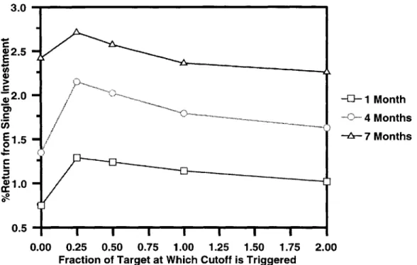
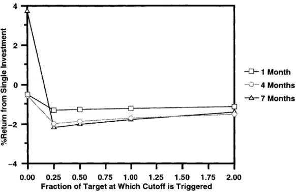
The expected returns from running the algorithm once under the assumptions that stocks could be bought or sold at any time and that D was known are shown in Figure 4-1.

It can clearly be seen that the algorithm yielded better returns when run on larger time periods and with tighter cutoffs. The complete results of running the algorithm under the

continuous assumption and various guesses for D can be seen in Table 4.1.

Guessing D

When the optimum return, D, was guessed, results were mixed. When D was guessed to

be the least of the results from other time periods, success rates rose slightly relative to

the results when D was known. When D was guessed to be the mean of the results from

other time periods, there were fewer successes. When the algorithm was run on longer time periods, the success rate for the mean guess was closer to that of the least guess and the case when D was known.

The expected return from a single investment fell when D was guessed. The mean guess almost always had a higher return than the least guess. Although the returns from a single investment were low when D was guessed to be the least of previous results, the annual return and the return combined with an alternate investment were higher. The least guess always outperformed the mean guess and almost always outperformed the known guess. When tight cutoffs were included, the least guess did outperform the known guess in every case. The mean guess always had lower annual returns and returns combined with the 30%

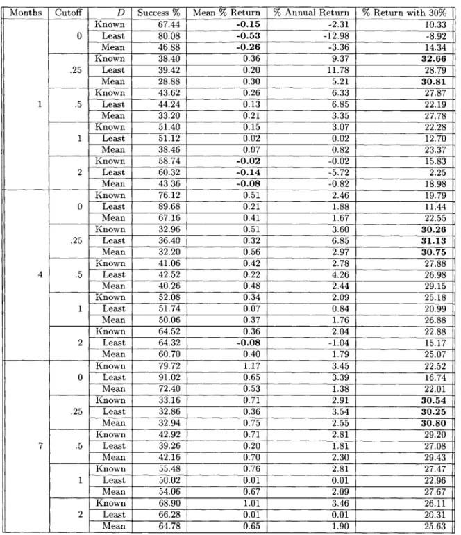
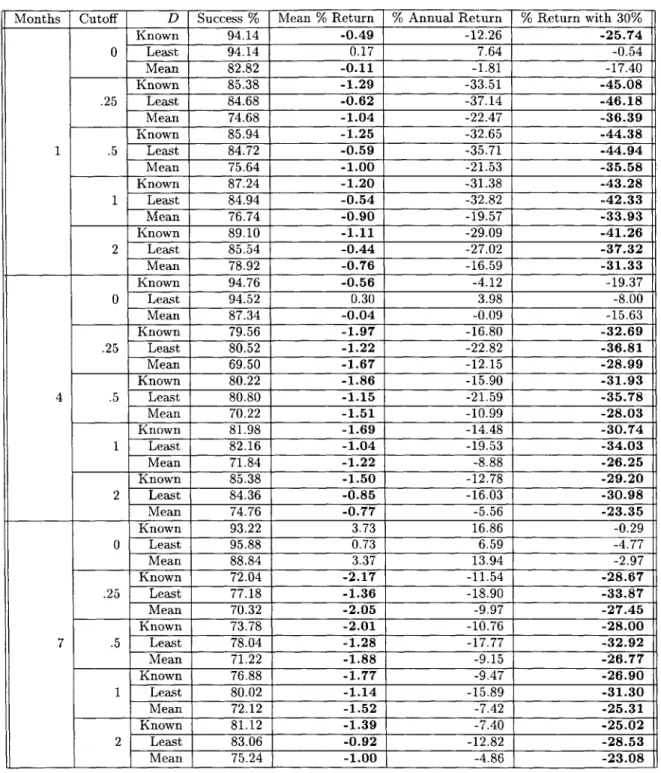
Months Cutoff D Success % Mean % Return % Annual Return % Return with 30% Known 92.44 0.75 21.74 47.92 0 Least 94.36 0.36 20.27 35.37 Mean 72.48 0.11 1.53 25.86 Known 82.74 1.29 48.57 86.02 .25 Least 84.46 0.65 66.61 98.34 Mean 66.10 1.06 22.86 55.68 Known 83.12 1.24 46.09 82.89 1 .5 Least 84.64 0.62 62.83 93.56 Mean 66.42 0.99 20.96 53.21 Known 83.80 1.14 41.56 76.98 1 Least 85.40 0.58 55.62 84.69 Mean 67.04 0.85 17.59 48.72 Known 86.02 1.02 35.47 68.73 2 Least 87.18 0.50 44.91 71.25 Mean 68.60 0.64 12.75 42.18 Known 92.76 1.35 9.29 35.54 0 Least 95.44 0.68 11.99 31.48 Mean 85.10 0.61 3.12 29.74 Known 72.34 2.15 18.12 51.62 .25 Least 79.60 1.16 32.56 66.86 Mean 63.98 1.78 10.57 42.21 Known 73.48 2.02 16.83 49.88 4 .5 Least 80.08 1.09 30.28 63.86 Mean 65.72 1.62 9.53 40.80 Known 75.36 1.79 14.65 46.85 1 Least 80.90 0.97 26.13 58.40 Mean 69.50 1.40 8.16 38.81 Known 81.66 1.63 13.00 44.12 2 Least 82.72 0.76 19.66 49.84 Mean 77.48 1.39 7.93 37.99 Known 95.24 2.42 9.85 37.93 0 Least 96.08 0.95 7.68 29.14 Mean 87.82 1.95 6.60 34.58 Known 70.40 2.71 12.56 45.04 .25 Least 73.80 1.54 17.92 50.65 Mean 66.98 2.53 9.51 41.28 Known 72.64 2.57 11.86 44.02 7 .5 Least 74.74 1.42 16.41 48.62 Mean 69.34 2.39 8.92 40.41 Known 76.24 2.36 10.72 42.34 1 Least 76.16 1.21 13.64 44.88 Mean 72.94 2.16 7.96 38.98 Known 83.02 2.26 10.09 41.06 2 Least 81.12 1.02 11.14 41.05 Mean 78.36 1.95 7.07 37.39 Table 4.1: Results tion

assump-3.0 02.5 -2.0 -4-1 _Month 4 Months E1 5 - -- 7 Months 0 1.0 0.5 0.00 0.25 0.50 0.75 1.00 1.25 1.50 1.75 2.00

Fraction of Target at Which Cutoff is Triggered

Figure 4-1: Expected return on a single investment under the continuous transaction as-sumption when D was known and the goal was to make money

investment than did the least guess or the case where D was known.

Results of the Control Group

In order to verify the effectiveness of the algorithm, the algorithm was run with random

stock selection. When the purchased stock was selected randomly, the number of successes dropped significantly. Although success levels were low, the random stock selection had a positive expected return in most cases. The return when combined with an alternate

investment, however, rarely exceeded the return of the alternate investment alone, and only at the tightest cutoff level. In all cases, the returns from the random stock selection were

smaller than those from the algorithm's choice.

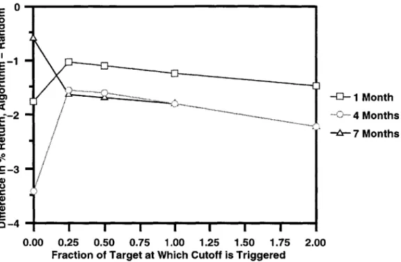
The difference in the expected return on a single investment under the continuous model

between the algorithm's choice and the random stock selection can be seen in Figure 4-2.

In every case, the algorithm's choice outperformed the random stock. The full results of random stock selection can be seen in Table 4.2.

Months Cutoff D Success % Mean % Return % Annual Return % Return with 30% Known 67.44 -0.15 -2.31 10.33 0 Least 80.08 -0.53 -12.98 -8.92 Mean 46.88 -0.26 -3.36 14.34 Known 38.40 0.36 9.37 32.66 .25 Least 39.42 0.20 11.78 28.79 Mean 28.88 0.30 5.21 30.81 Known 43.62 0.26 6.33 27.87 1 .5 Least 44.24 0.13 6.85 22.19 Mean 33.20 0.21 3.35 27.78 Known 51.40 0.15 3.07 22.28 1 Least 51.12 0.02 0.02 12.70 Mean 38.46 0.07 0.82 23.37 Known 58.74 -0.02 -0.02 15.83 2 Least 60.32 -0.14 -5.72 2.25 Mean 43.36 -0.08 -0.82 18.98 Known 76.12 0.51 2.46 19.79 0 Least 89.68 0.21 1.88 11.44 Mean 67.16 0.41 1.67 22.55 Known 32.96 0.51 3.60 30.26 .25 Least 36.40 0.32 6.85 31.13 Mean 32.20 0.56 2.97 30.75 Known 41.06 0.42 2.78 27.88 4 .5 Least 42.52 0.22 4.26 26.98 Mean 40.26 0.48 2.44 29.15 Known 52.08 0.34 2.09 25.18 1 Least 51.74 0.07 0.84 20.99 Mean 50.06 0.37 1.76 26.88 Known 64.52 0.36 2.04 22.88 2 Least 64.32 -0.08 -1.04 15.17 Mean 60.70 0.40 1.79 25.07 Known 79.72 1.17 3.45 22.52 0 Least 91.02 0.65 3.39 16.74 Mean 72.40 0.53 1.38 22.01 Known 33.16 0.71 2.91 30.54 .25 Least 32.86 0.36 3.54 30.25 Mean 32.94 0.75 2.55 30.80 Known 42.92 0.71 2.81 29.20 7 .5 Least 39.26 0.20 1.81 27.08 Mean 42.16 0.70 2.30 29.43 Known 55.48 0.76 2.81 27.47 1 Least 50.02 0.01 0.01 22.96 Mean 54.06 0.67 2.09 27.67 Known 68.90 1.01 3.46 26.11 2 Least 66.28 0.01 0.01 20.31 Mean 64.78 0.65 1.90 25.63

Table 4.2: Results of attempting to make money under the continuous assumption and random stock selection

E2.0

E

4

Fraction of Target at Which Cutoff is Triggered

Figure 4-2: Expected return on algorithm stock selection minus expected return on random stock selection under the continuous model when D was known and the goal was to make money

4.9.2 The Once-a-day Model

When running under the assumption that the algorithm could only buy and sell stock at the beginning of the day, the algorithm did not always make a profitable trade. Although its success rates were the same as those of the continuous model, the fact that it could only buy and sell stock at the beginning of the day prevented it from realizing the returns that the continuous model received. Often, even when it did make a profitable trade, the trade was insufficiently profitable for the algorithm combined with the alternate investment to outperform the alternate investment.

Much like in the continuous system, the algorithm had a higher expected return on a single investment in longer time periods. Again, successes in shorter time periods did much better than those in longer time periods when comparing annual returns and returns combined with the alternate investment. Cutoffs were almost completely detrimental. In-corporating cutoffs always reduced the expected return on a single investment. Generally, the tighter cutoffs had lower expected returns than the lax cutoffs. Although the cut-offs reduced the expected return on a single investment, they did increase the annual and

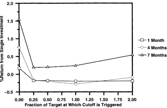
2.0 S1.5 E 1.0 _{-1- 1 Month} .4 Months E 0.5 -o- 7 Months W 0.0 -0 -0.5 0.00 0.25 0.50 0.75 1.00 1.25 1.50 1.75 2.00 Fraction of Target at Which Cutoff is Triggered

Figure 4-3: Expected return on a single investment under the once-a-day transaction as-sumption when D was known and the goal was to make money

combined returns slightly.

The expected returns from running the algorithm once under the assumptions that

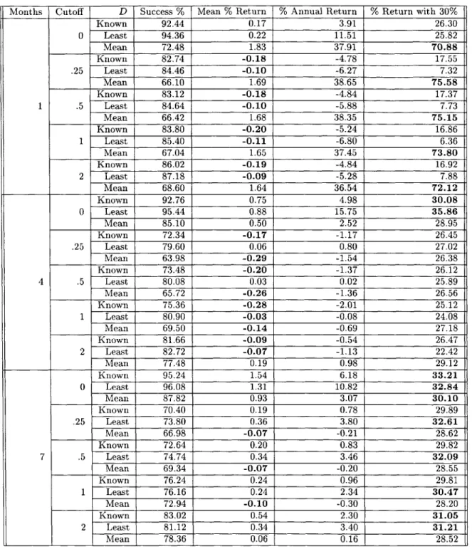
stocks could be bought or sold only at the beginning of the day and that D was known are shown in Figure 4-3. It can be seen that larger time periods and looser cutoffs had better returns. The complete results of running the algorithm under the once-a-day model and

with various guesses for D can be seen in Table 4.3.

Guessing D

When the optimum return, D, was guessed, results varied widely. When D was guessed

to be the mean of the results from other time periods and time periods were short, it consistently outperformed both the cases when D was known and D was guessed to be the

least result from other time periods. The mean guess outperformed the other two cases in

expected return from a single investment as well as annual return and combined return. For longer time periods, the reverse is true. The least guess generally outperformed the cases

where D was known and where D was the mean guess. The returns from the least guess in long time periods, however, were not as high as those of the mean guess in short time