Stability Improvement of the Interconnection of Weak AC Zones by Synchronverter-based HVDC link

HAL Id: hal-01387675

https://hal.archives-ouvertes.fr/hal-01387675

Submitted on 16 Nov 2016

HAL is a multi-disciplinary open access archive for the deposit and dissemination of sci-entific research documents, whether they are pub-lished or not. The documents may come from teaching and research institutions in France or abroad, or from public or private research centers.

L’archive ouverte pluridisciplinaire HAL, est destinée au dépôt et à la diffusion de documents scientifiques de niveau recherche, publiés ou non, émanant des établissements d’enseignement et de recherche français ou étrangers, des laboratoires publics ou privés.

Stability Improvement of the Interconnection of Weak

AC Zones by Synchronverter-based HVDC link

Raouia Aouini, Bogdan Marinescu, Khadija Ben Kilani, Mohamed Elleuch

To cite this version:

Raouia Aouini, Bogdan Marinescu, Khadija Ben Kilani, Mohamed Elleuch. Stability Improvement of the Interconnection of Weak AC Zones by Synchronverter-based HVDC link. Electric Power Systems Research, Elsevier, 2016. �hal-01387675�

1

1

Raouia AOUINI ²Bogdan MARINESCU 1Khadija BEN KILANI 1Mohamed ELLEUCH

1

Université de Tunis El Manar, Ecole Nationale d’Ingénieurs de Tunis, LR11ES15 Laboratoire des Systèmes Electriques, 1002, Tunis, Tunisie,

²SATIE-ENS Cachan, 61 Avenue du Président Wilson 94235 Cachan Cedex, France and IRCCyN-Ecole Centrale Nantes, BP 92101 • 1, rue de la Noë, 44321 Nantes Cedex 3

France

Email: aaouinii @yahoo.com, bogdan.marinescu@irccyn.ec-nantes.fr, khadijakilani @yahoo.fr, melleuch2008@gmail.com

Abstract-- The interconnection of weak electric power grids opens new issues into power system stability and control. This paper proposes a control strategy of HVDC transmission yielding increased power transfer capacity and enhanced transient stability of weak interconnected systems. The proposed control is a recently developed synchronverter-based control and emulation of the HVDC link (SHVDC). Methodologically, the transient stability of the neighbouring zone is a priori taken into account at the design level of the control. The parameters of the SHVDC regulators are tuned based on a specific residues method. The performances of the control strategy are analyzed by the power transfer limit

li mit

P when the interconnection is a pure DC link, and by both the Pli mit and the Critical

Clearing Time (CCT) when the interconnection is a hybrid DC/AC link. The study further investigates the impact of the inertia emulation that the synchronverter provides, and of the tuned control parameters on Pli mit. The proposed control is tested in comparison to the

standard vector control. The simulation results indicate that the synchronverter based control improves both the dynamic transfer capacity and the transient stability of weak interconnected power systems.

Keywords-- HVDC, synchronverter, stability limits, regulator parameters tuning.

Stability Improvement of the Interconnection of Weak AC

Zones by Synchronverter-based HVDC link

2 Nomenclature

V, E: Stator and grid voltages.

is, ig: Stator and grid currents.

e: Back emf.

P, Q: VSC active and reactive powers outputs. Ls, Rs: VSC inductance and resistance.

Lg, Rg: Grid inductance and resistance.

Zg: Grid impedance.

Cf: Filter capacitor.

Tm, Te: Mechanical and electromagnetic torques.

J: Inertia moment. θ : Rotor angle. M: Field excitation.

ω : Grid angular frequency.

V

Sac: Grid short circuit power.

PdN: rated DC power.

Dp , Dq: Frequency and Voltage droops.

s: Laplace operator. Subscript

G, M: SG and SM indices. 1. Introduction

The interconnection of AC electrical power grids have historically presented technical challenges ranging from frequency regulation, coordination of operations, and transient

3

stability [1]. These challenges have gained higher interest on one hand due to the incorporation of power electronic converters in the transmission links and on the other hand, due to the integration of weak, rather than strong power systems. In a weak system a small disturbance can cause large deviations in the voltage and other variables in the network. The short circuit level at a bus is commonly used as a measure of the system strength at that particular point. Technically, a weak AC system could be evaluated following several considerations: low ratio of inductance over resistance, high impedance and low inertia [2]. Examples of weak networks include isolated microgrids with renewable energy (wind power, photovoltaic...). Due to network weakness, dynamics of voltage and frequency are coupled, making it difficult to simultaneously guarantee voltage stability and frequency synchronization [2-4].

In response to these challenges, transmission in HVDC has been developed to mitigate these issues. The HVDC technology is able to provide to the transmission system advantages such as transfer capacity enhancement and power flow control [5]. Indeed, HVDC applications have widely increased, presenting diverse configurations: pure DC links or hybrid configurations where AC and DC circuits are parallelized. The strength of the AC system with respect to the power rating of the HVDC link is described by the Short-Circuit Ratio (SCR) [2-4]. The interconnected networks may be electrically strong AC systems with an SRC greater than 3, or weak networks suffering from low inertia and low SCR. Indeed, the HVDC links are increasingly used inside the same AC network in order to enhance the power transmission capacity between some zones of the grid, such as the integration of renewable energy distributed generators.

Many authors have investigated the impact of HVDC applications on stability limits of interconnected power systems [6-17]. For transient stability, the criteria used are the

4

Critical Clearing Time (CCT) and the power transfer limit Pli mit, called also the dynamic

transmission capacity in [18]. For pure HVDC links, only the criteria is used.

For parallel AC/DC lines, both the CCT and the Pli mit are used as transient stability

criteria: the CCT of a three-phase fault on the AC line, in addition to the total power transfer limit . The authors in [6-17] have shown that the strategy used to control the HVDC converters can impact the stability of the system in which the link is embedded. HVDC lines in parallel with HVAC lines are shown to improve the transient stability of power system quantified by the CCT. In a hybrid AC/DC link, increasing the DC power, improves the transient stability [17].

One of the main trends in control techniques for VSC-HVDC links is based on the well-known vector control scheme [9-15]. Despite the effectiveness of this control in many power converter applications, the use of the VSC-HVDC based on vector-current control in weak AC connections are claimed to exhibit low performances [19-23]. Reference [19] shows that using vector current control, the power limit of a VSC-HVDC link to an AC system with SCR = 1.0 is limited to only 0.4 p.u. Recently in [24], the synchronverter control has been adapted to the converters of a VSC-HVDC link. The concept of the synchronverter control is to mimic the behavior of a synchronous generator (SG) along with its voltage and frequency regulations [25]. The sending-end rectifier emulates a synchronous motor (SM) and the receiving end inverter emulates a synchronous generator (SG). The resulting Synchronverter based HVDC was called SHVDC [24].

This paper proposes a control strategy of HVDC transmission to increase power transfer capacity and enhance transient stability of weak interconnected systems. The proposed control is a synchronverter-based control and emulation of the HVDC link. Methodologically, the transient stability of the neighbouring zone is a priori taken into

li mit P li mit P li mit P

5

account at the design level of the control. The parameters of the SHVDC regulators are tuned by the sensitivity of the poles of the neighbouring zones of the HVDC to control parameters, and by the method of residues. The performances of the control strategy are analyzed by the power transfer limit Plimit when the interconnection is a pure DC link, and

by both the Pli mit and the Critical Clearing Time (CCT) when the interconnection is a

hybrid DC/AC link. The impact of the control parameters and the inertia emulation on the dynamic transmission capacity of an HVDC connection of two weak AC zones is firstly analyzed in a two weak terminals HVDC line. Second, we test the influence of the HVDC relative capacity on the stability limits in the case of a hybrid DC/AC interconnection. The proposed control is tested in comparison to the standard vector control. The simulation results indicate that the synchronverter based control improved both the dynamic transfer capacity and the transient stability of weak interconnected power systems.

The rest of the paper is organized as follows: in Section 2, the SHVDC structure is recalled. In Section 3, we present the criteria for transient stability. The tuning method of the proposed controller is developed in Section 4. Sections 4 and 5 present the simulation results.

2. Synchronverter-based HVDC connecting two weak AC systems 2.1 Characteristics of weak AC systems

The characteristics of AC systems have a significant impact on the operation of HVDC systems. The strength of an AC/DC system can be measured by its short circuit ratio (SCR) which is the ratio of the AC system short-circuit capacity to the rated power of the HVDC system. This is expressed in equation (1) [2]

ac dN S SCR P = , (1) li mit P

6

The short-circuit capacity of the grid at the PCC bus in Fig.1 is given by:

² ac g V S Z = , (2) The strength of an AC system may be quantified based on the classification given in [2-4]:

• Strong system, if the SCR of the AC system is greater than 3.0. • Weak system, if the SCR of the AC system is between 2.0 and 3.0. • Very weak system, if the SCR of the AC system is lower than 2.0.

Moreover, HVDC links connected to weak AC systems with low SCR have negative impacts on the AC system performances such as: power transfer limitations, voltage instability and high dynamic over-voltages.

2.2 Synchronverter based HVDC

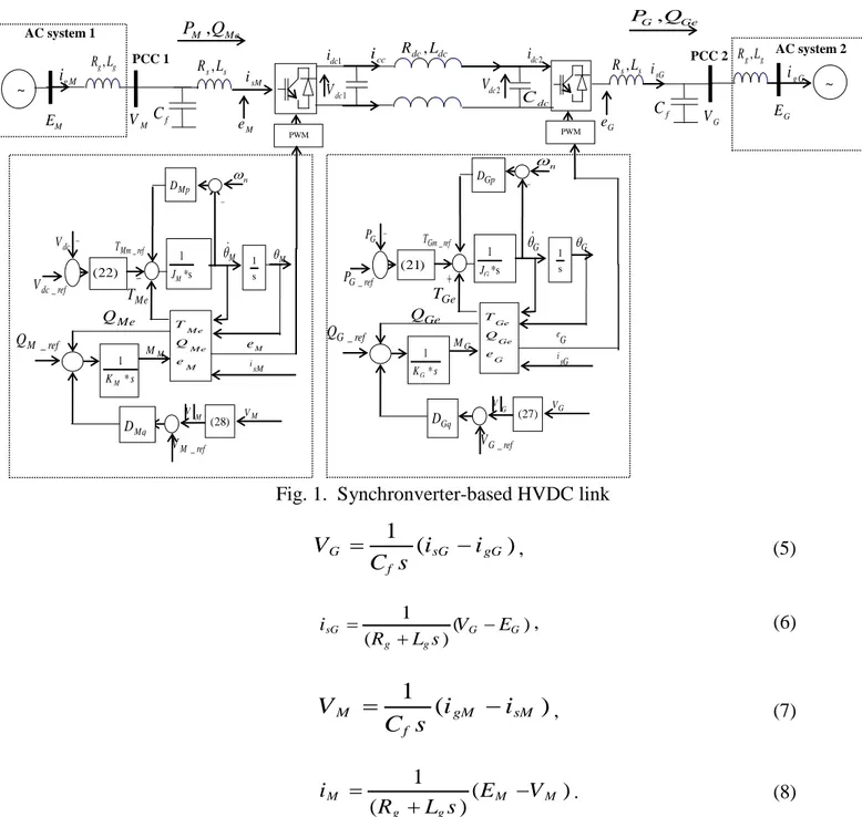
In this Section, the synchronverter-based emulation of HVDC link (SHVDC) is brievly recalled [24]. The SHVDC system consists of two synchronverters connected with a DC line as shown in Fig.1. The sending-end rectifier emulates a synchronous motor (SM) and the receiving end inverter emulates a synchronous generator (SG) [24]. Fig.1 depicts the power part of the SHVDC. It consists of an inverter/rectifier plus an LC filter. The basic equations of this circuit are expressed by (3) and (4).

sG G s sG s G di V R i L e dt = − − + , (3) sM M s sM s M di V R i L e dt = + + . (4) Each VSC converter is connected to the AC system (Fig.1) via a grid impedance representing the short-circuit power at the point of common coupling (PCC). The output current and voltage may be given by:

7

Fig. 1. Synchronverter-based HVDC link

1

(

)

V

i

i

C s

=

−

1

(

)

V

i

i

C s

=

−

As shown in Fig. 1, controllers include the mathematical model of a three-phase round-rotor synchronous machine described by [24]

1 ( ) G Gm Ge Gp G G T T D s J θ = − − θ _{, (9)} 1 ( ) M Me Mm Mp M M T T D s J θ = − − θ _{, (10)} n ω , g g R L AC system 1 M E , M Me P Q 1 dc V , s s R L , dc dc R L AC system 2 dc C sM i , G Ge P Q cc i ~ ~ PWM PCC 1 g M i M V M e f C 1 dc i idc2 2 dc V , s s R L sG i G e Cf PCC 2 G V , g g R L g G i G E G θ G θ n ω G P G M + Ge T − 1 *s G J Gp D Ge Ge G T Q e _ Gm ref T (21) 1 s e_G G V (27) Ge Q i sG Gq D _ G ref Q G V − _ G ref P 1 * G K s M θ M θ dc V M M − Me T − 1 *s M J Mp D Me Me M T Q e _ Mm ref T (22) 1 s M e M V (28) Me Q i sM Mq D _ M ref Q M V − _ dc ref V 1 * M K s PWM _ M ref V VG ref_

8 , Ge G sG G T =M <i sinθ >, (11) , Me M sM M T =M <i sinθ >, (12) sin G G G G e =M sθ  θ , (13) _ sin M abc M M M e =M sθ  θ , (14) , G G G sG G P =M sθ <i sinθ >, (15) , cos Ge G G sG G Q = −M sθ <i  θ >, (16) , cos Me M M sM M Q =M sθ <i  θ >, (17) , M M M sM M P =M s

θ

θ

2 2

sin sin sin( - ) sin( + )

3 3

T

π π

θ _{= } θ θ θ _

 

 , _{cos cos cos( -}2 _{) cos( +}2 ₎

3 3 T π π θ _{= } θ θ θ _    .

The operator <.,.>denotes the conventional inner product in �3. The frequency droop control loop of the SHVDC link is given by [24]

_ ( ) Gm Gm ref Gp n G T =T +D ω −sθ , (19) _ ( ) Mm Mm ref Mp n M T =T +D ω −sθ . (20) where Tgm_ref is the mechanical torque applied to the SG rotor, and it is generated by a PI

controller to regulate the real power output P_g (Fig. 1). It is expressed as

_ _ ( _ )( _ ) G G i p Gm ref p p G G ref k T k P P s = + − , (21) In the SM case, the reference torque Tmm_ref is generated by a DC voltage controller for

power balance [24]. _ _ _ 1 _ ( i vdc)( ) Mm ref p vdc dc ref dc k T k V V s = + − . (22)

9

The reactive power Qgm (respectively Qmm) is controlled by a voltage droop control loop

in order to regulate the field excitation Mg (respectively Mm)[24].

1 ( ) M Gm Ge G M Q Q k s = − , (23) 1 ( ) M Mm Me M M Q Q k s − = − , (24) G_ref ( _ ref ) Gm Gq G G Q =Q +D V −V (25) M_ref ( _ ) Mm Mq M ref M Q =Q +D V −V , (26) The output voltages amplitudes are computed by [24]

2

3(

V

V V

V V

V V

=

+

+

2

3(

V

V V

V V

V V

=

+

+

1 1 1 ( ) dc dc cc dc V i i C s = − , (29) 2 2 1 ( ) dc cc dc dc V i i C s = − , (30) Interconnected relationship between the two converters station is given by

1 2 cc dc dc dc cc dc di V V R i L dt = + + . (31) The AC and DC circuit equations have to be coupled. The coupling equations follow from the active power balance between AC and DC sides of each converter.

1 1 1 dc dc dc P =V i , (32) 2 2 2 dc dc dc P =V i , (33)

10 1 dc M P =P , (34) 2 dc G P =P . (35) Equation (31) could be expressed by

2 2 1 2 2 dc cc dc cc dc cc dc cc L di V i V i R i dt = + + (36) Combining the latter equation with (29), (30), the active power flow satisfies the equation : 2 2 2 2 1 2 1 1 2 2 ( ) 2 2 2 dc cc dc dc dc dc dc dc dc dc dc cc L di C dV C dV V i V i R i dt dt dt = + + + + (37)

From (37), the flow of active power in the HVDC transmission system is balanced, which means thatthe active power PM entering the HVDC system matches the active power

PG leaving it, plus the losses in the DC transmission system. Thus, (38) expresses this

power balance:

M G

P =P +losses .

(38) 2.3 Structural analysis of the SHVDC system

The scope of this Section is to analyze the SHVDC structure based on the algebraic approach [37] issued from dynamic systems theory. The latter consists in an analytic check of the degrees of freedom of the closed-loop (system along with regulations). The model of the SHVDC given by equations (3)-(35) is a general Differential Algebraic Equations (DAE) form. The approach introduced in [37] and related references can be directly used. In this latter, a linear systemΣis a module M defined by a matrix equation

( ) 0

S s w= , (39)

where S s( )is a matrix which elements are polynomials in the Laplace/derivation operator

11

For the SHVDC system, S s( ) results from the linear approximation of equations (3)-(35) and w is given by (40). The system in (39) is written in order to put into evidence the inputs of the controlled system, i.e., the variables which can be imposed by the controls.

Gc Ge Gm Gm_ref Me Mm Mm_ref Ge Gm dc1 dc1 dc1 Me Mm dc2 dc2 cc dc2 T _ _ _ _ _ _ _ _ w=[i ,V ,e ,i ,i ,V ,e ,i ,P , T ,T ,T ,θ ,P ,T ,T ,T ,θ ,Q ,Q ,M , V , V ,i ,P ,Q ,Q ,M , V ,V ,i ,i ,P , θ ,θ , , , , , , ] sG G gG sM M M gM G G M M G G M M

M ref G ref PG ref Vdc ref VM ref VG ref QM ref QG ref

 

. (40)

Let k= length (w) =40 and r=rank (S(s)) =32. From [37], the integer m= −k ris the rank of the moduleM , which coincides with the rank of the linear systemΣ. The number of

the independent inputs u=

{

}

which defines the system m=rank (M). For the SHVDC case, the rank of the module M defined by the SHVDC is equal to 8, which means that the number of the independent inputs is 8. The latter coincides with the references of the schemes in Fig. 1. More precisely, with given initial conditions, trajectories for the reference variables can be imposed by the controls.

Remark: In the SHVDC system in Fig.1, the power balance has been verified with

simulation: a step change of +0.3 p.u is applied to the reference power PG_ref . Fig.2 shows

that the power PM tracked the power PG, the responses of both powers tracked the set-point

PG_ref (modulo the losses). Thus, the line power is not changed in steady-state. From eq.

(37) and (38), the transient difference between PM and PG is stored in the Cdc capacitor of

the SHVDC line. More precisely, during the transient, the power balance is achieved using energy storage system in the HVDC link.

12

Fig.. 2 Responses of PM and PG to a +0.3 step in Pg_ref=0.4p.u

3. Transient stability criteria

Transient stability of a power system is defined as its the ability to maintain synchronism when subjected to a severe transient disturbance. In conventional transient stability studies, analysis aims at evaluating contingency severity in terms of stability limits. The stability limits of current concern are the power transfer limit for a given clearing time and the CCT for given pre-fault operating conditions [18, 29].

For a fault applied under given operating conditions, the CCT is defined as the maximal fault duration for which the system remains transiently stable [29]. The instability is then manifested by the loss of synchronism of a group of machines.

The power transfer limit considered here refers to the maximum flow of power that can be transmitted through a given flow gate (like, e.g., a line) for which the system remains dynamically stable after being subjected to a disturbance. The evaluation of the

depends on the initial operating condition as well as on the nature of the disturbance. Small disturbances are in the form of small load, generation or regulation set points variations and the system must be able to successfully transmit the power transfer limit noted limit

small

P _{under these disturbances [29]. The latter is the small signal stability margin of}

the system. Severe transient disturbances usually considered are short-circuits on buses or transmission lines. In this case, the power transfer limit is lower. We denote this limit

15 20 25 30 0 0.1 0.2 0.3 0.4 0.5 0.6 0.7 0.8 0.9 1 Time (sec) PM PG PM PG li mit P li mit P li mit P

13

limit

transient

P _{and it is a transient stability margin of the system which depends on the duration of}

the considered short-circuit. Obviously, the latter should be below the CCT [18].

The applications of HVDC transmission have considerable impact on stability limits of interconnected power systems [6-17]. For pure HVDC links as the example in Fig. 1, only the criteria is used. For parallel AC/DC lines (Fig. 13), the CCT of a three-phase fault on the AC line, measures the transient stability margin of the interconnected power systems, in addition to the total power limit . For both cases, the HVDC link is based on the synchronverter concept presented in Section 2. From [24] the standard parameters of the SG cannot be directly used for this structure. Thus, a specific tuning method of these parameters to enhance the stability limits and to satisfy the usual HVDC control requirements is discussed in the next section.

4. Control model description

The tuning methodology of the SHVDC parameters developed in [24] is briefly recalled. In the present work, the aforementioned tuning method is adopted for the interconnection of two weak AC systems having equal SRC=1 by VSC-HVDC link.

4.1 HVDC Control Specifications

The tuning procedure starts by defining the full set of control specifications for a VSC-based HVDC. In order to guarantee the set-points of the transmitted active power, the reactive power and the voltage at the points of coupling, their transient behaviour are tracked with the following transient performance criteria [27]:

-the response time of the active/reactive power is normally in the range of 50 ms to 150 ms; -the response time for voltage is about 100 ms to 500 ms.

li mit P

li mit P

14 4.2 Control objectives

In [24], a tuning methodology of the SHVDC parameters has been developed. The synthesis of the SHVDC parameters takes into account poorly damped oscillation modes of the neighbouring AC zone of the HVDC link. As a consequence, the stability limit in terms of the CCT of the neighbouring zone was improved in addition to the local performances presented above. The local performances for active and reactive power tracking are ensured [24]. More precisely, the synthesis of the SHVDC parameters is done such that the stability performances is ensured for several cases of fault (i.e, the enhancement of the stability limits based on the power limit and the CCT) along with the local ones. In this case, the impact of the SHVDC control parameters and the inertia emulation on the power limit is analyzed. The latter is computed for small and transient signals disturbances. A hybrid HVAC/HVDC line test power system will be used in Section 5.

4.3 Control Structure

In order to satisfy the cited control objectives, the SHVDC parameters should be tuned simultaneously and in a coordinated way. For this tuning, a feedback control presented in Fig.3 is applied on the system in Fig.1 where ∑ is modeled by (3)–(35) with the exception of (19), (20), (21), (22), (23), and (24).

All control parameters are grouped in the following diagonal matrix:

_ _

( , ) ( gp, mp , p V dc, i _V dc, gq, mq, p pg, i_ )pg

K s q =diag D D K K D D K K (41)

where D_gp, D_mp are, respectively, the static frequency droop coefficients of the SG and the

SM; D_gq,D_mqare, respectively, the voltage droop coefficient of the SG and of the SM;

_dc p V

K , _{_}

dc i V

K are the DC voltage PI control parameters; and _{_}

g

p P

K , _{_}

g

i P

K are the active

power PI control parameters.

li mit P

li mit P

15

Fig. 3. Feedback system

Note that all elements of the matrix K s q are tuned via the pole placement presented in ( , ) the following Section to meet HVDC performance specifications given in Section 4.1.

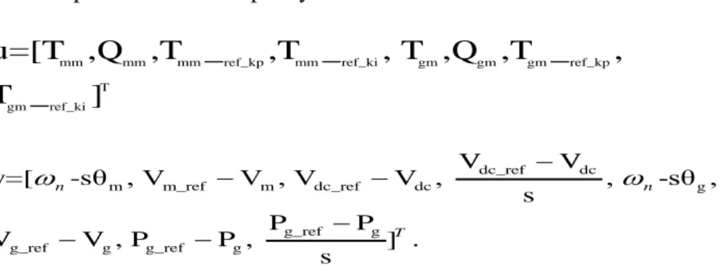
The inputs u and the outputs y are

mm mm mm ref_kp mm ref_ki gm gm gm ref_kp T gm ref_ki u=[T ,Q ,T _ ,T _ , T ,Q ,T _ , T _ ] dc_ref dc m m_ref m dc_ref dc g g_ref g g_ref g g_ref g V V y=[ -sθ , V V , V V , , -sθ , s P P V V , P P , ] . s n n T ω − − − ω − − −

4.4 Parameters and residues of the Regulators

The tuning of the control parameters is based on the poles sensitivity to the regulators parameters. The tuning design of the SHVDC controller is developed using the linear approximation of the feedback system in Fig.3 (HVDC-VSC and its control system) around an equilibrium point. The latter is a steady state operating point of the system in Fig.1 satisfying the usual linearization conditions which avoid variable limitations (like saturations…) and singular operating conditions. Let H s( )be the transfer matrix of a linear

approximation of ∑ and consider each closed-loop of the feedback system which corresponds only to input u and output _i y (see Fig.3). More specifically, _i H_ii( )s andK_ii( )s

are the (i,i) transfer functions of H(s), K s q( , ), respectively. The sensitivity of a pole

λ

( , ) ii K s q r q λ q λ ∂ ∂ ₌ ∂ ∂ (42) e _∑ ( , ) K s q u u’ y +

16

where rλ is the residue of Hii( )s at pole

λ

( , ) 1 ii s K s q q _=λ ∂ ₌ ∂ 4.5 Coordinated Tuning of SHVDC Parameters

First, desired locations *

i

λ can be computed for each pole λ_i starting from the control specifications given in Section 4.1. Table 1 summarizes the dynamics of interest and their associated modes. In fact, in Table 1; column 1 gives the dynamics of interest (for Pm, Qm,

Pg, Qg). Column 2 presents the initial mode associated with 0

i

λ of each dynamic of interest. Column 3 gives the desired mode associated with λi* of each dynamic of interest. The

criteria used to evaluate the dynamics of interest are based on the participation factors given in Table 2. The latter presents only the highest participation factor for each dynamics of interest in the associated mode. Therefore each dynamic is associated to only one pole for the computation of desired poles *

i

λ . From the same column of Table 2; several poles have also significant participations to the same dynamic which led us to compute the gains K in a coordinated way. More specifically, ifΛdenotes the set indices j from 1 to 8 for which

( )

jj

H s has

λ

0 i i ij j j r K λ λ ∈Λ = +

∑

λ is the initial (open-loop) location of the poleλi and rij is the residue of Hjj( )s

in λ_i . Finally, the pole placement is the solution of the following optimization problem

2 * * { , 1...8} arg min j j i i K i K j = =

∑

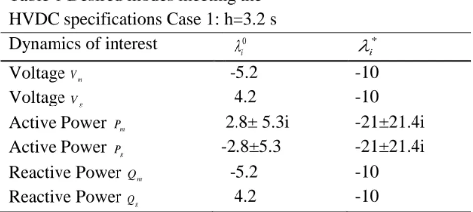
17 Table 1 Desired modes meeting the

HVDC specifications Case 1: h=3.2 s

Table 2 Participation factors Case 1: h=3.2 s

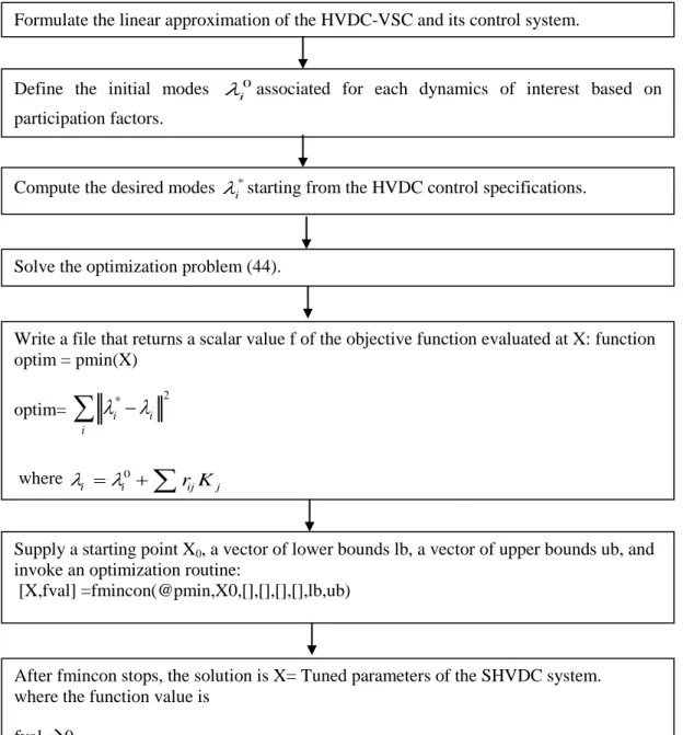
where λ_i is given by (43). The used optimization tool is based on the constrained nonlinear solver fmincon of Matlab Optimization Toolbox. The flow chart of the tuning parameters approach for the SHVDC converters is given in Fig. 4.

4.6 Simulations Results

In this Section, we consider is a pure VSC-HVDC link interconnection of two very weak AC systems, having SCR=1. The simulation method of the VSC converters is based on the average value model (AVM). The AVM approximates system dynamics by neglecting switching details [30]. The AVM of the VSCs consists of equivalent voltage sources generating the AC voltage averaged over one cycle of the switching frequency [30]-[32]. The average-value VSC-HVDC model used in the simulations is rated at ±100 kV, 200 MVA. The detailed system data is given in the appendix.

Dynamics of interest 0

i

λ λ i*

Voltage Vm -5.2 -10

Voltage Vg 4.2 -10

Active Power Pm 2.8± 5.3i -21±21.4i

Active Power Pg -2.8±5.3 -21±21.4i

Reactive Power Qm -5.2 -10 Reactive Power Qg 4.2 -10 % Pa V_ _m/Q_m Pa_Pm _{_ /} g g a V Q P _{_} g a P P 0 / m m V Q λ 41.29 34.1 0.34 0.16 0 m P λ 29 66.66 0.15 0.22 0 / g g V Q λ 0.16 0.2 31.06 42.57 0 g P λ 0.25 0.2 34.9 57.35

18

Fig. 4. Flow chart of the tuning SHVDC parameters

The optimal SHVDC parameters in the second column of Table 3 were obtained with (41) solved for the desired locations in Table 1. The new controller is compared with the standard vector controller. The latter has a cascade structure with an inner loop faster than the outer one. The proportional and integral gains of this control are tuned to satisfy the same performance specifications given in Section 4.1.

Formulate the linear approximation of the HVDC-VSC and its control system.

Define the initial modes 0

i

λ associated for each dynamics of interest based on participation factors.

Compute the desired modes λ_i*starting from the HVDC control specifications.

Write a file that returns a scalar value f of the objective function evaluated at X: function optim = pmin(X) optim= 2 * i i i λ λ−

∑

∑

Solve the optimization problem (44).

Supply a starting point X0, a vector of lower bounds lb, a vector of upper bounds ub, and

invoke an optimization routine:

[X,fval] =fmincon(@pmin,X0,[],[],[],[],lb,ub)

After fmincon stops, the solution is X= Tuned parameters of the SHVDC system. where the function value is

19 Table 3 SHVDC parameters

For the two controllers, small-signal and the transient stability margins, respectively

lim

small

P _and lim

transient

P _{, are evaluated using Matlab/Simulink toolbox. In the simulations, the}

limitations in DC current as well as DC voltages are taken into account, by saturations introduced in the PI controllers. In our case, the rated DC current and DC voltage are, respectively, 2 kA and ±100 kV. The maximum DC current is chosen 3.5 kA, so that the VSC valves currents will not exceed their acceptable current limits [33, 34]. The maximum limit of the DC voltage is chosen 1.5 p.u of the rated voltage as in [35-36].

A) Small-signal stability margin

A small step change is applied to different reference levels Pg_ref of the active power

transmitted through the HVDC link (see (21)). The limit

small

P _{is the maximum value of Pg_ref for}

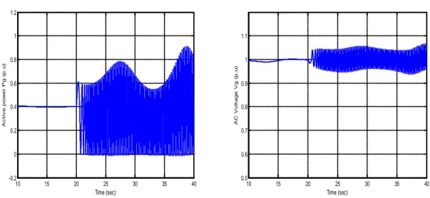
which the system remains dynamically stable after a small step change. Fig.5 shows the responses of the HVDC link of Fig.1 with the standard vector control. Fig.5.a presents steady-state responses of the system and instability after + 0.05 p.u step change to the active power reference Pg ref_ =0.4 p.u in 20 s. Similar tests shown in Fig.6 with lower values for

_

g ref

P _{led to stable responses. Thus} limit

small

P _{=0.39 p.u when the standard vector control is used.}

K SHVDC optimal

parameters for case 1

SHVDC optimal parameters for case 2

mp D _{15.06 10.38} mq D _{84.12 84.07} _dc p V K _{0.38 0.41} _dc i V K _{0.87 0.81} gp D _{200.8 250.52} gq D _{375 400} _g p P K _{32.33 30.27} _g i P K _{20.45 24.35}

20

(a) (b)

Fig. 5 Responses with vector control to a +0.05 step in Pg_ref=0.4p.u (p.u). (a) Response ofPg ;

(b) Response of Vg .

(a) (b)

Fig. 6 Responses with vector control to a +0.05 step in Pg ref_ =0.33(p.u) (a) Response ofPg to a

+0.05 step in Pg ref_ (p.u) ; (b) Response of Vg .

Second, responses of the SHVC link of Fig.1 with the new tuned parameters are

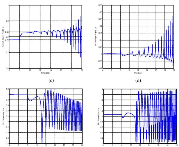
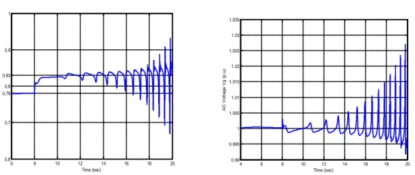
presented in Fig.7. The latter shows steady-state responses of the system and instability after + 0.05 p.u step increase in the active power reference Pg ref_ =0.78 p.u. Stable responses of the SHVDC are illustrated in Fig.8.

10 15 20 25 30 35 40 -0.2 0 0.2 0.4 0.6 0.8 1 1.2 Time (sec) A c ti v e pow er P g ( p. u) 10 15 20 25 30 35 40 0.5 0.6 0.7 0.8 0.9 1 1.1 Time (sec) A C V ol tage V g ( p. u) 10 15 20 25 30 35 40 0.25 0.26 0.27 0.28 0.29 0.3 0.31 0.32 0.33 0.34 0.35 0.36 0.37 0.38 0.39 0.4 Time (sec) A c t iv e pow er P g ( p. u) 10 15 20 25 30 35 40 0.985 0.99 0.995 1 1.005 Time (sec) A C V ol t age V g ( p. u)

21

(a) (b)

(c) (d)

Fig. 7 Responses of SHVDC to a +0.05 step in Pg_ref for the operating point of Pg = 0.78 p.u and H=

3.2 s. (a) Response of Pg; (b) Response of Vg ; (c) Response of Vdc; (d) Response of Vm.

(a) (b)

Fig. 8 Responses of SHVDC to a +0.05 step in Pg_ref for the operating point of Pg = 0.72 p.u and H=

3.2 s. (a) Response ofPg; (b) Response of Vg .

6 8 10 12 14 16 18 20 0,6 0,7 0.78 0,8 0.83 0,9 1 Time (sec) A c ti v e pow er P g ( p. u) 4 6 8 10 12 14 16 18 20 0.99 0.995 1 1.005 1.01 1.015 1.02 1.025 1.03 1.035 Time (sec) A C V ol tage V g ( p. u) 4 6 8 10 12 14 16 18 20 -0.8 -0.6 -0.4 -0.2 0 0.2 0.4 0.6 0.8 1 1.2 Time (sec) D C V ol tage V dc ( p. u) 4 6 8 10 12 14 16 18 20 0 0.2 0.4 0.6 0.8 1 1.2 1.4 1.6 1.8 2 Time (sec) A C V ol tage V m ( p. u) 7.7 7.8 7.9 8 8.1 8.2 8.3 8.4 8.5 8.6 8.7 0,6 0,62 0,64 0,66 0,68 0,7 0,72 0,74 0,76 0.77 0,78 0,8 Time (sec) A c ti v e pow er P g ( p. u) 7.6 7.8 8 8.2 8.4 8.6 8.8 9 9.2 0.997 0.998 0.999 1 1.001 1.002 1.003 Time (sec) A C V ol tage V g ( p. u)

22

The same rationale as above proves that the SHVDC structure enables a power transfer limit lim it

small

P _{of approximately 0.77 p.u. The latter is greater than the one obtained with the}

vector control. As a consequence, the SHVDC control improves the dynamic power transmission capacity of an HVDC link which connects two weak AC systems.

B) Transient signal margin

The total fault clearing time consists of the relay time and the breaker-circuit interrupting time [29]. On high voltage (HV) transmissions systems, the normal relay times range from 35 to 70 ms and the breaker-circuit interrupting times range from 70 to 130 ms.

In this study, a three phase short-circuit is applied at the point of common coupling, labeled PCC2 in Fig.1. The limit

transient

P _{is the maximum power through the DC link for which}

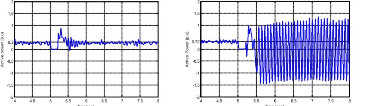
the system remains transiently stable after the clearing of the short-circuit. A 200 ms duration of the short-circuit was chosen for the tests.First, when the VSC-HVDC link uses vector control, the limit

transient

P _{is only 0.3 p.u (Fig.9.a), and the system is unstable when}

operating at a higher power than 0.3 p.u (Fig.9.b).

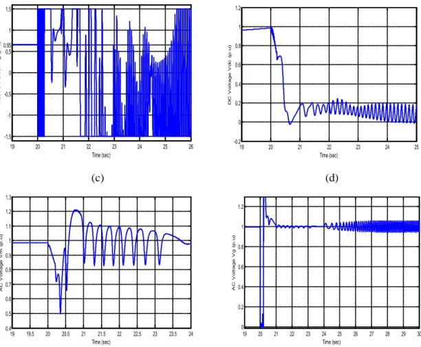
Second, the responses of the SHVDC system are presented in Fig. 10. The latter shows stable responses to a 200 ms short circuit with a power transfer of Pg = 0.64 p.u. However,

Figs. 11 show unstable responses of the SHVDC system with a power transfer of 0.65 p.u to the same fault. Therefore, the power transfer limit limit

transient

P _{is 0.64 p.u. The latter is}

greater than the one obtained with the vector control. This confirms the previous result on small signals margin stability of the system in Fig.1. Note also, that for the same controller, the limit

transient

P _{is smaller than the} limit

small

P _{. This is because the power transfer limit depends on}

the type of fault.

23

Fig. 9 Active power responses with the vector control to a 200 ms short-circuit and SCR = 1.0. (a) Response of Pg for Pg ref_ =0.3 .p u ; (b) Response ofPg for Pg ref_ =0.32 .p u.

(a) (b)

(c) (d)

Fig.10 Responses of SHVDC to a 200 ms short circuit for the operating point of Pg = 0.64 p.u. (a)

Response ofP ; (b) Response of Vg dc ; (c) Response of Vg; (d) Response of Vm.

(a) (b) 4 4.5 5 5.5 6 6.5 7 7.5 8 -2 -1,5 -1 -0,5 0 1 1,5 2 0.3 Time'sec) A c ti v e pow er ( p. u) 4 4.5 5 5.5 6 6.5 7 7.5 8 -2 -1.5 -1 -0.5 0 1 1.5 2 0.32 Time (sec) A c ti v e P ow er ( p. u) 19 19.5 20 20.5 21 21.5 22 22.5 23 -1,5 -1 -0,5 0 0,5 0.64 1 1,5 Time (sec) A c ti v e P ow er P g ( p. u) 19 20 21 22 23 24 25 0 0.5 1 1.5 Time (sec) D C V ol t age V dc ( p. u) 19 19.5 20 20.5 21 21.5 22 22.5 23 -10 -5 0 5 10 15 20 Time (sec) A C V ol tage V g ( p. u) 19 20 21 22 23 24 25 0 0.5 1 1.5 2 2.5 Time (sec) A C V ol t age V m ( p. u)

24

(c) (d)

Fig. 11 Responses of SHVDC to a 200 ms short circuit for the operating point of Pg = 0.65 p.u. (a)

Response ofPg; (b) Response of Vdc ; (c) Response of Vg; (d) Response of Vm.

C) Effect of the inertia emulation

The advantage of the SHVDC structure is to mimic the closed-loop of a standard synchronous generator. Thus inertia emulation is provided, and it is well known that the inertia has a positive impact on the stability of AC systems [30]. For this reason, we have analyzed the SHVDC structure for two different inertia constants:

- case 1: H=3.2 s (case in Section 4.2). - case 2: H= 5s.

For the two cases, we have placed the poles of the closed-loop at the same desired locations of dynamics of interest (Table 1). For case 2, the obtained tuned SHVDC parameters K are given in the third column of Table 3.

19 20 21 22 23 24 25 26 -1,5 -1 -0,5 0 0,5 0.65 1 1,5 Time (sec) A c t iv e P ow er P g ( p. u) 19 20 21 22 23 24 25 -0.2 0 0.2 0.4 0.6 0.8 1 1.2 Time (sec) D C V ol t age V dc ( p. u) 19 19.5 20 20.5 21 21.5 22 22.5 23 23.5 24 0.4 0.5 0.6 0.7 0.8 0.9 1 1.1 1.2 1.3 Time (sec) A C V ol t age V m ( p. u) 19 20 21 22 23 24 25 26 27 28 29 30 0 0.2 0.4 0.6 0.8 1 1.2 Time (sec) A C V ol t age V g ( p. u)

25 Table 4

Desired modes meeting the HVDC specifications Case 2: h=5s

Fig.12 shows that the system SHVDC of case 2 is unstable for Pg-ref magnitude just

greater than 0.78 p.u. As a consequence, the for case 2 is equal also to 0.77 p.u as for case 1. We can thus conclude that the improvement of the power transfer limit is due to the control manner (the way the closed-loop poles are placed) and not to the inertia emulation provided by the SHVDC structure.

5. Hybrid HVAC-SHVDC link test power system

In this Section, the specific tuning of the SHVDC parameters presented in Section 4.1 is tested on the hybrid HVAC-SHVDC interconnection shown in Fig. 13. As for the case of the two-bus system in Fig.1, the two AC zones are very weak, having equal SCR=1.

The two systems are connected with an AC line in parallel with one HVDC link. The 100 km HVDC cable link has a rated power of 200 MW and a DC voltage rating of ±100 kV. Each area consists of two identical generating units of 400 MVA/20 kV rating. Each of the units is connected through transformers to the 100 kV transmission line. There is a power transfer of 400 MW from Area 1 to Area 2. The detailed system data is given in the appendix. The control SHVDC approach is assessed for stability limits based on the CCT and the , defined in Section 3.

li mit P li mit P li mit P Dynamics of interest 0 i λ * i

λ

Active Power Pm 5.1± 8.3i -21±21.4i -0.03 ±0.1i

Active Power Pg -1.8±8.3 -21±21.4i -0.01 ± 0.1i

Reactive Power Qm 2.6 -10 -0.5

26

(a) (b)

Fig. 12 Responses of SHVDC to a +0.05 step in Pg_ref for the operating point of Pg = 0.78 p.u and

H= 5 s. (a) Response of Pg; (b) Response of Vg .

Fig 13. Hybrid HVAC-SHVDC interconnection

In this Section, only the transient stability margin limit

transient

P _{of the interconnected system is}

investigated. In the following, the influence of the relative capacity of the HVDC and the parallel AC transmission is investigated. The ratio between the active power transmitted and the continuous power to HVDC line is defined by

ac dc P P

ρ = , (45) where Pac is the per unit active power transmitted by the AC line and Pdc is the continuous

per unit power of the DC line. According to [17], the strength of an AC line may be quantified by the value of ρ:

-ρ ≥ 1.5: the AC line is strong -ρ ≤ 0.7: the AC line is weak

6 8 10 12 14 16 18 20 0,6 0,7 0.78 0,8 0.83 0,9 1 Time (sec) A c ti v e pow er P g ( p. u) 4 6 8 10 12 14 16 18 20 0.99 0.995 1 1.005 1.01 1.015 1.02 1.025 1.03 1.035 Time (sec) A C V ol tage V g ( p. u) DC Line Turbine Pt Control System Qv Control System Pt Control System G1 G2G2 Pac Pdc Turbine Qv Control System

27

The objective of this study is to investigate the impact of the ratio ρ on the stability limits in the case of hybrid HVAC-SHVDC interconnection.

5.1 Results of the CCT with different ρ

The reference per unit power of the DC line Pg_ref presented in equation (21) is varied

(Pg_ref = 0.2, 0.4, 0.6, 0.8, 1, 1.2 and 1.3) keeping constant the total transmitted power:

T dc ac

P = P + P constant = . (46) The obtained CCTs for a three-phase short-circuit fault in the mid-point of the AC transmission line are presented in Table 5 for different DC power levels. From Table 5, the increase of the DC power reduces the AC power transfer capability and improves therefore the CCT. We can see from Table 5 that the SHVDC control with new tuned parameters improves the transient stability of the system and thus augments the transient stability margins of the neighbouring AC zone when the AC line becomes weaker. This is due to the fact that the DC power is increased, and that the dynamics of the neighbour zone are taken into account at the synthesis stage via the oscillatory modes in Table 2. The gains of the controllers are computed not only for the local HVDC dynamics, but also to damp oscillatory modes and diminish the general swing of the zone. Moreover, it is noted that for each value of Pg_ref, the gains K of the SHVDC controller are not recomputed and are thus

the same as in the appendix. This result confirms the robustness test in [29] of the performances of the proposed controller against variation of operating conditions.

5.2 Results of the lim

transient

P _{with different}

In this Section, the total power limit limit

transient

P _{given in (46) is evaluated for different per}

unit DC powers Pg_ref (Pg_ref = 0.2, 0.4, 0.6, 0.8, 0.85, 0.9, 1, 1.2 and 1.3).

28 Table 5 CCT with different DC power

To evaluate the power transfer limit limit

transient

P of the interconnection, a short-circuit of 200 ms duration (which is below to the CCTs computed for all DC power levels (see Table 5)) is applied in the middle of the AC line.It is noted that the power limit limit

transient

P _{is the}

maximum power through the two parallel lines for which the system remains stable after the short-circuit. The results in Table 6 and Fig. 14 show that limit

transient

P _{is proportional to the}

DC power. However, this latter reaches a maximum value called the optimal power limit

lim

Poptimit . We can see that the transient stability margin of the parallel HVAC/HVDC line is

reduced when the power limit is greater than the . As a result, for the hybrid HVAC/HVDC transmission lines, the increase of the DC power of the HVDC line above this threshold could not improve any longer the power limit of the interconnection, whereas the increase of the DC power improves the transient stability of the interconnected power system without any constraint. From Table 5, we can note the optimal DC power transferred by the HVDC Poptim

dc =0.85 p.u which corresponds to the power limit = 1.8

p.u. lim Poptimit lim Poptimit DC Power Pg_ref (p.u) AC power Pac (p.u) ac dc P P ρ= CCT (ms) 0.2 1.32 6.6 210 0.4 1.12 2.8 240 0.6 0.92 1.53 260 0.8 0.72 0.9 290 1 0.52 0.52 310 1.2 0.32 0.23 340 1.3 0.22 0.17 355

29 Table 6 The power limit levels lim

transient

P _with

different DC power levels

Fig.14 The power limit lim

transient

P

with different DC power levels 6. Conclusion

This paper proposed a control strategy of HVDC transmission yielding increased power transfer capacity and enhanced transient stability of weak interconnected systems. The proposed control is based on the synchronverter control and emulation of the HVDC link (SHVDC).

The transient stability of the neighbouring zone is a priori taken into account at the design level of the control. The parameters of the SHVDC regulators are tuned based on a specific residues method. The control strategy has been tested for two configurations of interconnection of two very weak AC zones: an HVDC line and a hybrid HVAC-HVDC interconnection. In the former, the performance of the control strategy is analyzed by the power limit Plimit . In the latter, both the Pli mit and the Critical Clearing Time (CCT) are

used. For these configurations, better results than with the vector current control were obtained:

(i) Better dynamic performances, since this approach allows one to analytically take into account dynamic specifications at the tuning stage.

0,2 0,3 0,4 0,5 0,6 0,7 0,8 0.85 0,9 1 1,1 1,2 1,3 1,38 1.4 1.45 1.5 1.55 1.6 1.65 1.7 1.75 1.8 Pdc (p.u) P lim it tr ans ei nt ( p. u) Pdc optim=0.85 p.u Plimit optim= 1.8 p.u

DC Power Pg_ref (p.u) AC power Pac (p.u) ac dc P P ρ= lim transient P 0.2 1.31 6.55 1.48 0.4 1.11 2.77 1.65 0.6 0.91 1.51 1.72 0.8 0.71 0.88 1.79 0.85 0.66 0.78 1.8 0.9 0.61 0.67 1.78 1 0.51 0.51 1.75 1.2 0.31 0.25 1.55 1.3 0.22 0.09 1.42

30

(ii) Better dynamic transmission capacity of the HVDC connection of two weak AC zones in the sense that the link capacity under stability constraints is higher than the one obtained when using the standard vector control. This improvement of the dynamic transmission power is due to the way by which the SHVDC parameters are tuned and not to the inertia emulation provided by the SHVDC structure.

(iii) Better stability margins have been obtained for both interconnection cases: hybrid HVAC/SHVDC or only SHVDC. Swing information is directly taken into account at the synthesis stage in terms of the less damped modes of the neighbouring zone and not only for the local HVDC dynamics as it is the case for the standard VSC control.

The exploitation of the proposed control in weak interconnected systems may be more advantageous in low-inertia systems which have limited number of rotating machines, or no machines at all. Examples of such applications can be found when an HVDC link is powering island applications or if it is connected to renewable generators.

7. References

[1] P. Kundur , J. Paserba ; V. Ajjarapu ; G. Andersson ; A. Bose ; C. Canizares ; N. Hatziargyriou ; D. Hill ; A. Stankovic ; C. Taylor ; T. Van Cutsem ; V. Vittal, ‘’ Definition and Classification of Power System Stability’’, IEEE Transactions on Power Systems, 2004, Vol: 19, Issue: 3, pp: 1387 – 1401.

[2] “IEEE guide for planning DC links terminating at AC locations having low short circuit capacities,” IEEE Std 1204-1997, Tech. Rep., 1997.

[3] B. Franken and G. Andersson, “Analysis of HVDC converters connected to weak systems,” IEEE Trans. Power Syst., vol. 5, no. 1, pp. 235–242, February 1990.

[4] A. Gavrilovic, “AC/DC system strength as indicated by short circuit ratios,” in AC/DC Power Transmission International Conference, London, 1991.

[5] D. Murali, M. Rajaram, and N. Reka, “Comparison of FACTS devices for power system stability enhancement,” Int. J. Comput. Applicat., vol. 8, no. 4, 2010, 0975–8887.

[6] Vovos, N.A., Galanos, G.D.: ‘Enhancement of the transient stability of integrated AC/DC systems using active and reactive power modulation’, IEEE Power Eng. Rev.., 1985, 5, (7), pp. 33–34.

[7] Smed, T., Andersson, G.: ‘Utilizing HVDC to damp power oscillations’, IEEE Trans. Power Deliv., 1993, 8, (2), pp. 620–627.

[8] Hammad, A.E., Gagnon, J., McCallum, D.: ‘Improving the dynamic performance of a complex AC/DC system by HVDC control modifications’, IEEE Trans. Power Deliv., 1990, 5, (4), pp. 1934–1943.

li mit P

31

[9] Shun, F.L., Muhamad, R., Srivastava, K., Cole, S., Hertem, D.V., Belmans, R.: ‘Influence of VSC HVDC on transient stability: Case study of the Belgian grid’. Proc. IEEE Power and Energy Society General Meeting, 25–29 July 2010, pp. 1–7.

[10] Taylor, C.W., Lefebvre, S.: ‘HVDC controls for system dynamic performance’, IEEE Trans. Power Syst., 1991, 6, (2), pp. 743–752.

[11] Latorre, H.F., Ghandhari, M., Söder, L.: ‘Control of a VSC-HVDC operating in parallel with AC transmission lines’. Proc. Transmission and Distribution Conf. and Exposition IEEE, Latin America, 2006, pp. 1–5.

[12] Henry, S., Despouys, O., Adapa, R., et al.: ‘Influence of embedded HVDC transmission on system security and AC network performance’. Cigré, 2013.

[13] To, K., David, A., Hammad, A.: ‘A robust co-ordinated control scheme for HVDC transmission with parallel AC systems’, IEEE Trans. Power Deliv., 1994, 9, (3), pp. 1710–1716.

[14] Latorre, H., Ghandhari, M.: ‘Improvement of power system stability by using a VSC-HVDC’, Int. J. Electr. Power Energy Syst.., 2011, 33, (2), pp. 332–339.

[15] D. Jovcic, L. Lamont, and L. Xu, “VSC transmission model for analytical studies,” in Proc. IEEE Power Eng. Soc. General Meeting, Toronto, Canada, 2003.

[16] A.E. Hammad, Stability and control of HVDC and AC transmission in parallel, IEEE Trans. Power Deliv. 14 (4) (1999) 1545–1554.

[17] R. Aouini, K. Ben Kilani, B. Marinescu and M. Elleuch « Improvement of fault critical clearing time by HVDC transmission », The 9th International Muti-Conference on Signals, Systems, Devices , SSD’2011, pp. PES-, Sousse, 22-25 Mars 2011. (Tunisia).

[18] M. Pavella, D. Ernst, and D. Ruiz-Vega, Transient Stability of Power Systems: A Unified Approach to Assessment and Control, ser. Kluwer International Series in Engineering and Computer Science. New York, NY, USA: Springer, 2000.

[19] M. Durrant, H. Werner, and K. Abbott, “Model of a VSC HVDC terminal attached to a weak ac system,” in Proc. IEEE Conf. Control Applications, Istanbul, Turkey, 2003.

[20] L. Pilotto, M. Szechtman, A. Hammad, "Transient AC Voltage Related Phenomena for HVDC Schemes Connected to Weak AC Systems", IEEE Trans., PWRD, July 1992, pp. 1396-1404.

[21] P. Fischer, “Modelling and control of a line-commutated HVDC transmission system interacting with a VSC STATCOM,” Ph.D. dissertation, Royal Inst. Technol., Stockholm, Sweden, 2007.

[22] L. Zhang, L. Harnefors, and H.-P. Nee, “Power-synchronization control of grid-connected voltage-source converters,” IEEE Trans. Power Syst., vol. 25, no. 2, pp. 809–820, May 2010.

[23] L. Zhang and H.-P. Nee, “Multivariable feedback design of VSC-HVDC connected to weak AC systems,” in Proc. PowerTech 2009, Bucharest, Romania, 2009.

[24] R. Aouini, B. Marinescu, K. Ben Kilani and M. Elleuch" Synchronverter-based Emulation and Control of HVDC transmission", IEEE Trans. Power Syst., Jan. 2016, Vol. 31, Issue: 1 Pages: 278 – 286.

[25] Q.-C. Zhong, and G.Weiss, "Synchronverters: Inverters that mimic synchronous generators," IEEE Trans. Ind. Electron., Apr. 2011, vol. 58, no. 4, pp. 1259–1267.

32

[27] S. Li, T.A. Haskew, and L. Xu, , "Control of HVDC light system using conventional and direct current vector control approaches," IEEE Trans. Power Electr., 2010, 25, (12), pp. 3106–3118.

[28] R. Aouini, B. Marinescu, K. Ben Kilani and M. Elleuch « Improvement of transient stability in an AC/DC system with synchronverter based HVDC» The 12th International Muti-Conference on Signals, Systems, Devices , SSD’2015, pp. PES-, Mahdia, 16-19 Mars 2015 (Tunisia).

[29] P. Kundur, Power System Stability and Control. New York, NY, USA: McGraw-Hill, 1994.

[30] S. Chiniforoosh, J. Jatskevich, A. Yazdani, V. Sood, V. Dinavahi, J. A. Martinez, and A. Ramirez, “Definitions and Applications of Dynamic Average Models for Analysis of Power Systems”, IEEE Trans. on Power Delivery, vol. 25, no. 4, pp. 2655–2669, Oct. 2010..

[31] A. Yazdani and R. Iravani, “Dynamic model and control of the NPC based back-to-back HVDC systems,” IEEE Trans. Power Del., vol. 21, no. 1, pp. 414–424, Jan. 2006.

[32] J. Peralta, H. Saad, S. Dennetière, and J. Mahseredjian, “Dynamic performance of average-value models for multi-terminal VSC-HVDC systems,” Proc. IEEE Power Eng. Soc. Gen. Meeting, SanDiego, CA, 2012. [33] M. Callavik, A. Blomberg, J. Häfner, and B. Jacobson, “The Hybrid HVDC Breaker - An innovation breakthrough enabling reliable HVDC grids,” ABB Grid Systems Technical Paper, Nov. 2012.

[34] Matthias K. Bucher, and Christian M. Franck, “Contribution of Fault Current Sources in Multi-Terminal HVDC Cable Networks’’, IEEE Transactions on Power Delivery, Vol. 28, No. 3, July 2013.

[35] Alireza Nami, Jiaqi Liang, Frans Dijkhuizen, Peter Lundberg’’ Analysis of modular multilevel converters with DC short circuit fault blocking capability in bipolar HVDC transmission systems’ Power Electronics and Applications (EPE'15 ECCE-Europe), 2015 17th European Conference.

[36] K. R. Padiyar , ‘’HVDC Power Transmission Systems: Technology and System Interactions’’, page 104-130, John Wiley & Sons Inc (August 1991).

[37] H. Bourlès, B. Marinescu, "Linear-Time Varying Systems, Algebraic-Analytic Approach", Springer-Verlag, LNCIES 410, 2011.

8. Appendix Network data (Fig. 1)

Bus system 1 & 2: line voltage=230 kV, frequency=50 Hz, Short circuit power=200 MVA, Rs=0.75Ω , Ls=0.2 H. Generators G1, G2: Rated 200 MVA, 100/230 kV

DC system: voltage= ±100 kV, rated DC power=200 MW,

Pi line R=0.0139 Ω /km, L=159 µH/km, C=0.331 µF/km, Pi line length= 150 km, DC capacitor=0.005 F, smoothing reactor: R=0.0251Ω , L= 100mH.

Parameters of the classic vector control: current loop: kp=5, ki=1, AC voltage control: ki=20, active power control: ki=20, DC voltage control: kp=5, ki=2.

Tuned of the the SHVDC parameters for SHVDC interconnection (Fig. 1) Network data (Fig. 13)

Generators G1, G2: Rated 200 MVA, 20 kV

Xl (p.u): leakage Reactance = 0.18, Xd (p.u.): d-axis synchronous reactance = 1.305, T’d0 (s): d-axis open circuit sub-transient time constant =0.296, T’d0 (s): d-axis open circuit transient time constant = 1.01

33

Xq (p.u): q-axis synchronous reactance = 0.053, Xq (p.u): q-axis synchronous reactance = 0.474, X’’q (p.u): q-axis sub-transient reactance =0.243, T’’q0 (s): q-axis open circuit sub transient time constant=0.1

M =2H (s): Mechanical starting time = 6.4

Governor control system: R (%): permanent droop =5, servo-motor: ka = 10/3, ta (s) = 0.07, regulation PID: kp = 1.163, ki= 0.105, kd= 0

Excitation control system: Amplifier gain: ka = 200, amplifier time constant: Ta (s) = 0.001, damping filter gain kf = 0.001, time constant te (s) = 0.1

Generator transformers Rated 400 MVA, 20/ 100 kV , Coupling Delta/ Yg Primary resistance (p.u) =0.002, Primary inductance (p.u) =0.12

Secondary resistance (p.u) =0.002, Secondary inductance (p.u) =0.12 Loads: PL1=200 MW, PL2= 1GW

AC transmission lines

Resistance per phase (Ω/km) =0.03, Inductance per phase (mH/km) =0.32, Capacitance per phase (nF/km) =11.5

Tuned of the the SHVDC parameters for the hybrid HVAC-SHVDC interconnection (Fig. 13) K= [ 55; 46.4; 24.0 ; 28.5 ; 65.64; 58.069; 56.39; 25.11; 37.35].