Diagnosis in Infinite-State Probabilistic Systems (long version)

(1)

HAL Id: hal-01334218

https://hal.inria.fr/hal-01334218

Submitted on 20 Jun 2016

HAL is a multi-disciplinary open access

archive for the deposit and dissemination of

sci-entific research documents, whether they are

pub-lished or not. The documents may come from

teaching and research institutions in France or

abroad, or from public or private research centers.

L’archive ouverte pluridisciplinaire HAL, est

destinée au dépôt et à la diffusion de documents

scientifiques de niveau recherche, publiés ou non,

émanant des établissements d’enseignement et de

recherche français ou étrangers, des laboratoires

publics ou privés.

version)

Nathalie Bertrand, Serge Haddad, Engel Lefaucheux

To cite this version:

Nathalie Bertrand, Serge Haddad, Engel Lefaucheux. Diagnosis in Infinite-State Probabilistic Systems

(long version). [Research Report] Inria Rennes; LSV, ENS Cachan. 2016. �hal-01334218�

(2)

(long version)

Nathalie Bertrand

1

_{, Serge Haddad}

2

_{, and Engel Lefaucheux}

1,2

1 Inria, France nathalie.bertrand@inria.fr 2 LSV, ENS Cachan & CNRS & Inria, France

{serge.haddad,engel.lefaucheux}@ens-cachan.fr

Abstract

In a recent work, we introduced four variants of diagnosability (FA, IA, FF, IF) in (finite) probabil-istic systems (pLTS) depending whether one considers (1) finite or infinite runs and (2) faulty or all runs. We studied their relationship and established that the corresponding decision problems are PSPACE-complete. A key ingredient of the decision procedures was a characterisation of diagnosability by the fact that a random run almost surely lies in an open set whose specification only depends on the qualitative behaviour of the pLTS. Here we investigate similar issues for infinite pLTS. We first show that this characterisation still holds for FF-diagnosability but with a Gδ set instead of an open set and also for IF- and IA-diagnosability when pLTS are finitely branching. We also prove that surprisingly FA-diagnosability cannot be characterised in this way even in the finitely branching case. Then we apply our characterisations for a partially ob-servable probabilistic extension of visibly pushdown automata (POpVPA), yielding EXPSPACE procedures for solving diagnosability problems. In addition, we establish some computational lower bounds and show that slight extensions of POpVPA lead to undecidability.

1 Introduction

Diagnosis. Monitoring (hardware and/or software) systems prone to faults involves several

critical tasks: controlling the system to prevent faults as much as possible, deducing the cause of the faults, etc. Most of these tasks assume that an observer has the capability to assess the

status of the current run based on the outputs of the system: providing information about

the possible occurrence of faults. Such an observer is called a diagnoser and its associated task is called diagnosis. This framework leads to interesting decision and synthesis problems: “Does there exist a diagnoser?” and in the positive case “How to build such a diagnoser?”, “Which kind of diagnoser is sufficient?”, etc. The decision problem, on which we focus here,

is called diagnosability [14].

Diagnosis of discrete event systems. In order to formally reason about diagnosability, the

systems were first modelled by finite labelled transition systems (LTS). Then the specification of a diagnoser is defined by two requirements: correctness, meaning that the information provided by the diagnoser is accurate, and reactivity, ensuring that a fault will eventually be detected. Within the framework of finite LTS, the decision problem was shown to be solvable in PTIME [9] and it is in fact NLOGSPACE-complete.

Diagnosis of probabilistic systems. A natural way of modelling partially observable

systems consists in introducing probabilities (e.g. when the design is not fully known or the effects of the interaction with the environment is not predictible). Thus the notion of diagnosability was later extended to Markov chains with labels on transitions, also called probabilistic labelled transition systems (pLTS) [15]. In this context, the reactivity requirement now asks that faults will be almost surely eventually detected. Regarding correctness, two specifications have been proposed: either one sticks to the original definition

Leibniz International Proceedings in Informatics

(3)

and requires that the provided information is accurate, defining A-diagnosability; or one weakens the correctness by admitting errors in the provided information that should, however, have an arbitrary small probability defining AA-diagnosability. From a computational viewpoint, we recently proved that A-diagnosability is PSPACE-complete [3] and that AA-diagnosability can be solved in PTIME [4].

In case a system is not diagnosable, one may be able to control it, by forbidding some controllable actions, so that is becomes diagnosable. This property of active diagnosability has been studied for discrete-event systems [13, 8], and for probabilistic systems [2]. Interestingly, the diagnosability notion in the latter work slightly differs from the original one in [15]. Building on this variation, in [3] semantical issues have been investigated and four relevant notions of diagnosability (FA, IA, FF, IF) have been defined depending on (1) whether one considers finite or infinite runs and (2) faulty or all runs. In finite pLTS, it was shown that all these notions can be characterized by the fact that a random run almost surely lies in an open set, whose specification only depends on the qualitative behaviour of the pLTS.

Diagnosis of infinite-state systems. Diagnosability in infinite-state systems has been studied, on the one hand for restricted Petri nets [5], for which an accurate diagnoser can be designed, and on the other hand for visibly pushdown automata (VPA) [11], for which diagnosability can be decided via the determinisation procedure of [1]. However to the best of our knowledge diagnosis of probabilistic infinite-state systems has not yet been studied.

Contributions. The characterisations of diagnosability established in [3] strongly relied

on the finiteness of the models. Our first aim is thus to establish characterisations in the infinite-state case. FF-diagnosability (the original notion of diagnosability) states that almost surely a faulty run will be detected in finite time. We establish that FF-diagnosability can be characterised by the fact that a random run almost surely lies in a Gδ set, only

depending on the qualitative behaviour of the system. This characterisation also applies to IF-diagnosability for finitely-branching systems, since then the two notions coincide. An

ambiguous infinite correct (resp. faulty) run is a run indistinguishable from a faulty (resp.

correct) run. IA-diagnosability states that almost surely a run is unambiguous. The set of ambiguous runs is an analytic set (so a priori not known to be a Borel set). However in the finitely-branching case, we establish that the set of unambiguous runs is a Gδ set,

yielding a characterisation of IA-diagnosability. FA-diagnosability states that the probability that a finite run is unambiguous goes to 1 when its length goes to infinity. Surprisingly, despite the fact that IA-diagnosability and FA-diagnosability are very close, we prove that FA-diagnosability cannot be characterised by the fact that a random run almost surely lies in a Gδ set. Furthermore we strenghten this result by another inexpressivess result also related

to FA-diagnosability.

We then introduce partially observable probabilistic visibly pushdown automata (POpVPA), a model generating infinite-state probabilistic systems. We show how to exploit the above characterisations to design a decision procedure for diagnosability in POpVPA. More precisely we show that we can “encode” our characterisations in an enlarged probabilistic VPA and then exploit the decision procedures of [7] leading to an EXPSPACE algorithm. Since our characterisations are not regular, this requires some tricky machinery. Finally we complete this work by exhibiting an EXPTIME lower-bound and showing that slight extensions of POpVPA lead to undecidability of the diagnosability problem.

Organisation. In Section 2, we successively introduce probabilistic infinite-state systems,

equip them with partial observation and faults, and define diagnosability notions. In Section 3, we establish characterisations of the diagnosability notions and inexpressiveness results. We exploit the characterisations to design decision procedures for POpVPA in Section 4, also

(4)

proving hardness and undecidability results. We conclude and give some perspectives in Section 5. All the proofs are given in Appendix.

2 Diagnosis specifications of infinite-state probabilistic systems

2.1 Probabilistic labelled transition systems

Probabilistic labelled transition systems (pLTS) are labelled transition systems equipped with probability distributions on transitions outgoing from a state.

▸Definition 1. A pLTS is a tupleM = ⟨Q, q0, Σ, T, P⟩ where:

Q is a finite or countable set of states with q0∈ Q the initial state;

Σ is a finite set of events;

T ⊆ Q × Σ × Q is a set of transitions;

P∶ T → Q_>0 is the transition probability fulfilling: ∀q ∈ Q, ∑_(q,a,q′_)∈TP[q, a, q′] = 1.

Given a pLTSM, the transition relation of the underlying LTS L is defined by qÐ→ qa ′ for (q, a, q′) ∈ T; this transition is then said to be enabled in q. In order to emphasise the relation between the pLTS and the LTS, we sometimes writeM = (L, P). Note that since we assume the state space to be at most countable, a pLTS is by definition at most countably branching: from every state q, there are at most countably many transitions enabled in q.

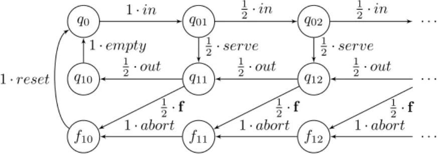
▸Example 2. The pLTS of Figure 1 represents a server that accepts jobs (event in) until it

randomly decides to serve the jobs (event serve). When a job is done the result is delivered (event out). When all jobs are done, the server waits for a new batch of jobs. However randomly, the server may trigger a fault (event f ) and then abort all remaining jobs (event

abort). Afterwards, the server is reset (event reset). In the figure, the label of a transition

(q, a, q′_{) is depicted as P[q, a, q}′_{] ⋅ a.} q0 q10 f10 q01 q11 f11 q02 q12 f12 . . . . . . . . . 1⋅ in 1₂⋅ in 1₂⋅ in 1 2⋅ out 1 2⋅ out 1 2⋅ out

1⋅ empty 1₂⋅ serve 1₂⋅ serve

1⋅ abort 1⋅ abort 1⋅ abort

1 2⋅ f 1 2⋅ f 1 2⋅ f 1⋅ reset Figure 1 An infinite-state pLTS.

Let us now introduce some important notions and notations that will be used throughout the paper. A run ρ of a pLTS M is a (finite or infinite) sequence ρ = q0a0q1. . . such that

for all i, qi ∈ Q, ai ∈ Σ and when qi₊₁ is defined, qi ai

Ð→ qi₊₁. The notion of run can be

generalised, starting from an arbitrary state q. We write Ω for the set of all infinite runs of M starting from q0, assuming the pLTS is clear from context. When it is finite, ρ ends in

a state q and its length, denoted∣ρ∣, is the number of events occurring in it. Given a finite run ρ= q0a0q1. . . qn and a (finite or infinite) run ρ′= qnanqn+1. . ., we call concatenation of

ρ and ρ′and we write ρρ′the run q0a0q1. . . qnanqn+1. . .; the run ρ is then a prefix of ρρ′,

which we denote ρ⪯ ρρ′. The cylinder defined by a finite run ρ is the set of all infinite runs that extend ρ: C(ρ) = {ρ′∈ Ω ∣ ρ ⪯ ρ′}. Cylinders are a basis of open sets for the standard topology on the set of runs (which can be viewed as an infinite tree). One equips a pLTS

(5)

with a probability measure on Ω with σ-algebra beingB, the set of Borel sets, and which is uniquely defined by Caratheodory’s extension theorem from the probabilities of the cylinders:

P(C(q0a0q1. . . qn)) = P[q0, a1, q1]⋯P[qn−1, an−1, qn] .

We will sometimes omit the C and write P(ρ) for P(C(ρ)). It is well-known that once the measure is fixed, one can enlarge the set of of measurable sets by considering the smallest

σ-algebra containingB and the “null” sets: {A ∣ ∃B ∈ B A ⊆ B ∧ P(B) = 0} and then extend

the original measure to a (complete) measure on this enlarged σ-algebra. We consider this measure in the sequel.

The sequence associated with ρ = qa0q1. . . is the word σρ = a0a1. . ., and we write

indifferently qÐ→ρ∗ or qÐ→σρ ∗ (resp. qÐ→ρ∗q′or qÐ→σρ ∗q′) for an infinite (resp. finite) run ρ. A state q is reachable (from q0) if there exists a run such that q0

ρ

Ð→∗_{q, which we alternatively}

write q0Ð→∗q. The (infinite) language of pLTS M consists of all infinite words that label

runs ofM and is formally defined as Lω(M) = { σ ∈ Σω∣ q0

σ

Ð→∗_}.

2.2 Partial observation and faults

The observation of a pLTS is given by a mask function. This function projects every event to its observation. This observation is partial as an event can have no observation or shares its observation with another event, but it is deterministic.

▸Definition 3. A partially observable pLTS (POpLTS) is a tupleN = ⟨M, Σo,P⟩ consisting

of a pLTSM equipped with a mapping P ∶ Σ → Σo∪ {ε} where Σois the set of observations.

Note that our setting generalises most existing frameworks of fault diagnosis by considering a mask functionP onto a possibly different alphabet rather than a partition of the event alphabet into observable and unobservable events. An event a∈ Σ is said unobservable if P(a) = ε, fully observable if P(a) ≠ ε and P−1_{({P(a)}) = {a} and partially observable if}

P(a) ≠ ε and ∣P−1_{({P(a)})∣ > 1. The set of unobservable events is denoted Σ}_u_.

Let σ∈ Σ∗ be a finite word; its length is denoted∣σ∣. The mapping P is extended to finite words inductively: P(ε) = ε and P(σa) = P(σ)P(a). We say that P(σ) is the mask of σ. Write∣σ∣o for∣P(σ)∣. When σ is an infinite word, its mask is the limit of the masks of its

finite prefixes. This mask function is applicable to runs via their associated sequence; it can be either finite or infinite. As usual the mask function is extended to languages. With respect toP, a POpLTS N is convergent if there is no infinite sequence of unobservable events from any reachable state: Lω_{(M) ∩ Σ}∗_Σω

u = ∅. When N is convergent, for every σ ∈ Lω(M),

P(σ) ∈ Σω

o. In the rest of the paper we assume that POpLTS are convergent. P can also be

be viewed as a mapping from runs to Σω_o by definingP(q0a0q1a1. . .) = P(a0a1. . .). Remark

that this mapping is continuous. We will refer to a sequence for a finite or infinite word over Σ, and an observed sequence for a finite or infinite sequence over Σo. Clearly, the application

of the mask function onto Σo of a sequence yields an observed sequence.

The observable length of a run ρ denoted ∣ρ∣o∈ N ∪ {∞}, is the number of observable

events that occur in it: ∣ρ∣o = ∣σρ∣o. A signalling run is a finite run whose last event is

observable. Signalling runs are precisely the relevant runs w.r.t. partial observation issues since each observable event provides an additional information about the execution to an external observer. Given states q, q′ and an observed sequence σ∈ Σ+_o, we write qÔ⇒ qσ ′ if there is a signalling run from q to q′with observed sequence σ.

In the sequel starting from the initial state q0, SR denotes the set of signalling runs, and

SRn the set of signalling runs of observable length n. Since we assume that the POpLTS are

convergent, for all n> 0, SRnis equipped with a probability distribution defined by assigning

(6)

signalling subrun of ρ of observable length n. For convenience, we consider the empty run q0

to be the single signalling run, of null length.

2.3 Fault diagnosis for POpLTS

To model the problem of fault diagnosis in POpLTS, we assume the event alphabet Σ contains a special event f ∈ Σ called the fault. A run ρ is then said to be faulty if its associated sequence of events contains a fault, i.e. σρ∈ Σ∗f Σω; otherwise it is correct. The set of faulty

(resp. correct) runs is denoted F (resp. C). For n∈ N, we write Fn for the set of runs ρ such

that ρ_↓n is faulty and Cn for the set of runs ρ such that ρ_↓n is correct. By definition, for all

n, Ω= Fn⊎ Cn, F= ⋃n_∈NFn and C= ⋂n_∈NCn.

In order to reason about faults we partition sequences of observations into three subsets: an observed sequence σ ∈ Σωo is surely correct if P−1(σ) ∩ Lω(M) ⊆ (Σ ∖ f)ω; it is surely

faulty ifP−1(σ) ∩ Lω_{(M) ⊆ Σ}∗_f_Σω_{; otherwise, it is ambiguous. For finite sequences, we need}

to rely on signalling runs: a finite observed sequence σ∈ Σ∗o is surely faulty (resp. surely

correct) if for every signalling run ρ withP(σρ) = σ, ρ is faulty (resp. correct); otherwise

it is ambiguous. A (finite signalling or infinite) run ρ is surely faulty (resp. surely correct,

ambiguous) ifP(ρ) is surely faulty (resp. surely correct, ambiguous).

In order to specify various requirements for diagnosability we need to refine the notion of ambiguity. LetN be a POpLTS and n ∈ N with n ≥ 1. Then:

FAmb_∞ (resp. CAmb_∞) is the set of infinite faulty (resp. correct) ambiguous runs ofN ; FAmbn(resp. CAmbn) is the set of infinite runs ofN whose signalling subrun of observable

length n is faulty (resp. correct) and ambiguous;

At this point it is interesting to look at the status of the different subsets of runs we have introduced with respect to the Borel hierarchy. The complementary sets Fn and Cn are

unions of cylinders; so they are open (and by complementation) closed sets. The set of faulty (resp. correct) runs F (resp. C) is an open (resp. closed) set as a union (resp. intersection) of open (resp. closed) sets. The sets FAmbn and CAmbn are unions of cylinders; so they are

open. The sets FAmb_∞and CAmb_∞ may be defined as follows. Consider(Σ2o)ωand Ω2 both

equipped with the product topology. SameObs= {(ρ, ρ′) ∣ P(ρ) = P(ρ′)} is the inverse image by a continuous mapping of the closed set {(σ, σ) ∣ σ ∈ Σωo}. Therefore SameObs is closed.

Thus C× F ∩ SameObs is a Borel set. The first and second projections are exactly CAmb_∞ and FAmb_∞ which establishes that these sets are analytic sets (i.e. continuous images of Borel sets). The set of analytic sets is a strict superset of Borel sets but every analytic set is still measurable w.r.t. the complete measure [12, 2H8 p.83].

In the context of finite POpLTS, we introduced four possible specifications of diagnosab-ility [3]. There are two discriminating criteria: whether the non ambiguity requirement holds for faulty runs only or for all runs, and whether ambiguity is defined at the infinite run level or for longer and longer finite signalling subruns. LetN be a POpLTS. Then:

N is IF-diagnosable if P(FAmb∞) = 0.

N is IA-diagnosable if P(FAmb∞⊎ CAmb∞) = 0.

N is FF-diagnosable if lim supn_→∞P(FAmbn) = 0.

N is FA-diagnosable if lim supn_→∞P(FAmbn⊎ CAmbn) = 0.

We recall in the next theorem all the implications that hold between these definitions. Missing implications do not hold, already for finite-state POpLTS.

▸Theorem 4 ([3]). Let N be a POpLTS. Then

N FA-diagnosable ⇒ N IA-diagnosable and FF-diagnosable; N IA-diagnosable or FF-diagnosable ⇒ N IF-diagnosable;

(7)

If N is finitely branching, then N is IF-diagnosable iff N is FF-diagnosable.

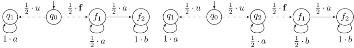
In order to illustrate the different kinds of diagnosability, we describe below some discriminating examples. q0 f1 f2 q1 1 2⋅ f 1 2⋅ a 1 2⋅ u 1 2⋅ a 1⋅ b 1⋅ a q0 q2 f1 f2 q1 1 2⋅ u 1 2⋅ f 1 2⋅ a 1 2⋅ u 1⋅ a 1 1⋅ b 2⋅ b 1 2⋅ a

Figure 2 Left: a POpLTS that is IF-diagnosable but not IA-diagnosable. Right: a POpLTS that

is IA-diagnosable but not FA-diagnosable.

Consider the POpLTSN on the left of Figure 2 where {u, f} is the set of unobservable events (represented by dashed arrows) andP is the identity over the other events. A faulty run will almost surely produce a b-event that cannot be mimicked by the single correct run. Thus this POpLTS is IF-diagnosable. The unique correct run ρ= q0uq1aq1. . . has

probability 1₂ and its corresponding observed sequence aω is ambiguous. Thus the POpLTS is not IA-diagnosable. This simple example shows that, already for finite-state POpLTS, IF-diagnosability does not imply IA-diagnosability.

Similarly, let us look at the POpLTS on the right of Figure 2 where{u, f} is the set of unobservable events andP is the identity over the other events. Any infinite faulty run will contain a b-event, and cannot be mimicked by a correct run, therefore FAmb_∞= ∅. The two infinite correct runs have aωas observed sequence, and cannot be mimicked by a faulty run, thus CAmb_∞= ∅. As a consequence, this POpLTS is IA-diagnosable. Consider now the infinite correct run ρ= q0uq1aq1. . .. It has probability 1₂, and all its finite signalling

subruns are ambiguous since their observed sequence is an, for some n∈ N. Thus for all

n≥ 1, P(CAmbn) ≥ 1₂, so that this POpLTS is not FA-diagnosable.

3 Characterisation of diagnosability

The aim of this section is to establish “simple” characterisations of the diagnosability notions for a POpLTSN = ((L, P), Σo,P) and more precisely to study whether one can express it

as a Borel set B∈ B only depending on the underlying LTS L and the mask function P, such that almost surely a random run belongs to B if and only ifN is diagnosable. Furthermore if possible, one looks for a set B belonging to a low level of the Borel hierarchy. Observe that for all notions, this requires some machinery since the finite runs-based notions FF and FA are expressed by a family of Borel sets and the infinite runs-based notions IF and IA are expressed by a set which is not a priori a Borel set.

Pursuing this goal, we introduce a language pathL for specifying Borel sets of runs. It is based on path formulae. A path formula α is a predicate over finite prefixes of runs. The (pseudo-)syntax of a formula of pathL is:

φ∶∶= α ∣ ¬φ ∣ φ1∧ φ2∣ ◇φ

where α is a path formula. In the sequel we use the standard shortcut◻φ ≡ ¬ ◇ ¬φ. A formula is evaluated at some position k of a run ρ= q0a0q1. . .. The prefix ρ[0, k] of ρ

is defined by ρ[0, k] = q0a0q1. . . qk. The semantics of pathL is inductively defined by:

ρ, k⊧ α if and only if α(ρ[0, k]); ρ, k⊧ ¬φ if and only if ρ, k /⊧ φ;

(8)

ρ, k⊧ φ1∧ φ2if and only if ρ, k⊧ φ1 and ρ, k⊧ φ2;

ρ, k⊧ ◇φ if and only if there exists k′≥ k such that ρ, k′⊧ φ.

Finally ρ⊧ φ if and only if ρ, 0 ⊧ φ. Due to the presence of path formulae (with no restriction) this language subsumes LTL and more generally any ω-regular specification language. In order to reason about the probabilistic behaviour of a POpLTS, we introduce qualitative probabilistic formulae P&p(φ) with & ∈ {<, >, =}, p ∈ {0, 1} and φ ∈ pathL. The semantics is obvious: N ⊧ P&p(φ) if and only if P_N({ρ ∈ Ω ∣ ρ ⊧ φ}) & p. Since pathL is closed by complementation the probabilistic formulae can be restricted to P=0(φ) and P>0(φ).

Let us give some examples of path formulae. Given a finite run ρ= q0a0q1. . . qk, let f

be defined by f(ρ) = true if ai = f for some index i. This path formula characterises the

faulty finite runs. Let U be defined by U(ρ) = true if there exists a correct signalling run ρ′ withP(ρ) = P(ρ′). Using the path formulae f and U, we exhibit a formula of pathL that characterises FF-diagnosability.

▸Proposition 5. Let N be a POpLTS. Then N is FF-diagnosable iff N ⊧ P=0(◇ ◻ (f ∧ U)).

Due to Theorem 4, in finitely-branching POpLTS the above characterisation also holds for IF-diagnosability. We also need the finitely-branching assumption in order to characterise IA-diagnosability. To this goal, let us introduce a more intricate path formula. For σ∈ Σ∗o,

we define firstf(σ) by firstf(σ) = min{k ∣ ∃ρ signalling run P(ρ) = σ ∧ ρ_↓k is faulty} with the convention that min(∅) = ∞. Then the path formula W is defined by: W(ε) = false and W(q0a0. . . qn₊₁) = true if firstf(P(q0a0. . . qn₊₁)) = firstf(P(q0a0. . . qn)) < ∞.

▸Proposition 6. Let N be a finitely branching POpLTS. Then N is IA-diagnosable iff

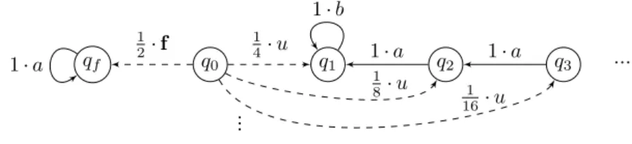
N ⊧ P=0_{(◇ ◻ (U ∧ W)).} q0 qf q1 q2 q3 ⋮ ⋯ 1 2⋅ f 1 4⋅ u 1 8⋅ u 1 16⋅ u 1⋅ a 1⋅ a 1⋅ a 1⋅ b

Figure 3 An infinitely-branching IA-diagnosable POpLTS.

The POpLTS of Figure 3 illustrates the necessity of the finitely-branching requirement in Proposition 6. {u, f} is the set of unobservable events and P is the identity over the other events. Observation b occurs in every infinite correct run, while the observed sequence of the single infinite faulty run is aω. This POpLTS is thus IA-diagnosable. However, it does not satisfy P=0(◇ ◻ (U ∧ W)) since the unique infinite faulty run has probability 12 and satisfies

◻U. Indeed for every n ∈ N, there is a correct signalling run with observed sequence an_.

Observe that the sets of runs specified by the characterisations of FF-diagnosability (◇ ◻ (f ∧ U)) and IA-diagnosability (◇ ◻ (U ∧ W)) are Fσ sets, i.e. countable unions of closed

sets. Surprisingly, we show that such a characterisation is impossible for FA-diagnosability.

▸Proposition 7. There exists a finitely-branching LTSL and a mask function P such that for every Fσ set E of runs, there exists a POpLTSN = ((L, P), Σo,P) such that:

either N is FA-diagnosable and P_N(E) > 0; or N is not FA-diagnosable and P_N(E) = 0.

(9)

We conjecture that the previous impossibility result also holds for all Borel sets. The next proposition shows that a positive probability condition (instead of a null condition) may not exist whatever the Borel set.

▸Proposition 8. There exists a finitely-branching LTSL and a mask function P such that for every Borel set E of runs, there exists a POpLTSN = ((L, P), Σo,P) such that:

either N is FA-diagnosable and P_N(E) = 0; orN is not FA-diagnosable and P_N(E) > 0.

4 Diagnosis for probabilistic pushdown automata

We now turn to a concrete model for infinite-state POpLTS, namely the ones generated by probabilistic pushdown automata, and more specifically by probabilistic visibly pushdown automata. Our goal is to use the characterisations from the previous section to decide the diagnosability of POpLTS generated by partially observable probabilistic visibly pushdown automata (POpVPA). To do so, we face the difficulty that the Borel sets that characterise IF-, IA- and IF-diagnosability are not a priori regular, even in the finite branching case. Yet, for POpVPA, we circumvent this problem, and manage to specify these sets by pLTL formula on a determinisation of the model, tagged with the needed atomic propositions. The decidability of the qualitative model checking for recursive probabilistic systems [7] then yields the decidability of the above three diagnosability notions for POpVPA.

4.1 Probabilistic visibly pushdown automata

Among probabilistic infinite-state systems the ones generated by probabilistic pushdown automata [10, 7] support relevant decision procedures. Already in the non-probabilistic case, the subclass of visibly pushdown automata (VPA) [1] is more tractable than the general model. In VPA, the type of events determines whether the operation on the stack is a push, a pop, or possibly changes the top stack symbol, so that the languages defined by VPA enjoy most of the desirable properties regular languages have.

▸Definition 9. A probabilistic visibly pushdown automaton (pVPA) is a tupleA = (Q, Σ, Γ, δ, P)

where:

Q is a finite set of control states with q0 the initial state;

Σ is a finite alphabet of events, partitionned into local, push and pop events Σ= Σ_♮⊎Σ_♯⊎Σ_♭. Γ is a finite alphabet of stack symbols including a set of bottom stack symbols Γ with initial symbol0∈ Γ;

δ⊆ Q × Γ × Σ × Q × Γ∗is the set of transitions such that for every (q, γ, a, q′, w) ∈ δ, ∣w∣ ≤ 2, γ∈ Γ implies w∈ Γ(Γ ∖ Γ)∗ and γ∉ Γ implies w∈ (Γ ∖ Γ)∗;

P is the transition probability function fulfilling for every q∈ Q and γ ∈ Γ:

∑(q,γ,a,q′,w_)∈δ P[(q, γ, a, q′, w)] = 1.

A transition t= (q, γ, a, q′, w) ∈ δ is said to be a local (resp. push, pop) transition if ∣w∣ = 1

(resp. ∣w∣ = 2, ∣w∣ = 0). We require that for every transition t = (q, γ, a, q′, w) ∈ δ, t is a local

(resp. push, pop) transition iff a is a local (resp. push, pop) event.

The semantics of a pVPA is an infinite-state pLTS whose states are pairs(q, z) consisting of a control state and a stack contents.

▸Definition 10. A pVPAV = (Q, Σ, Γ, δ, P) defines a pLTS M_V= (Q_V,(q0,0), Σ, TV, PV)

where:

(10)

T_V= {((q, zγ), a, (q′, zw)) ∣ zγ ∈ Γ(Γ ∖ Γ)∗∧ (q, γ, a, q′, w) ∈ δ};

For every ((q, zγ), a, (q′, zw)) ∈ T_V, P_V[((q, zγ), a, (q′, zw))] = P[(q, γ, a, q′, w)].

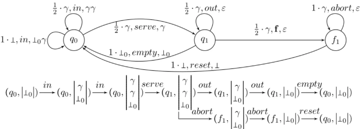
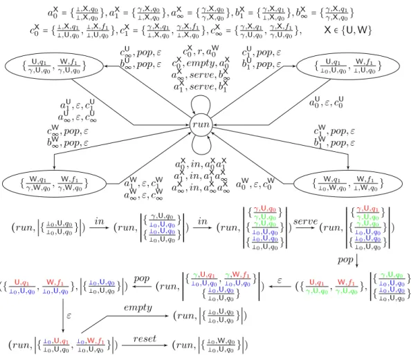
▸ Example 11. Figure 4 gives an example of a pVPA. The event alphabet is composed

of local events {serve, empty, reset}, a push event in and pop events {out, f, abort}. A transition t= (q, γ, a, q′, w) is represented by an edge from state q to state q′and labelled by

P[t] ⋅ γ, a, w. The semantics of this pVPA is precisely the pLTS from Figure 1. Indeed, the

stack alphabet consists of two letters Γ= {γ, 0} where the set of bottom stack symboll is

Γ= {0}. Thus one can encode the stack using a counter that gives the number of γ in the

stack. For instance, in the pLTS from Figure 1 the configuration(q1,0γn) of the pVPA

corresponds to the state q1n.

q0 q1 f1 1 2⋅ γ, serve, γ 1⋅ 0, empty,0 1 2⋅ γ, f, ε 1⋅ , reset, 1 2⋅ γ, in, γγ 1⋅ , in, 0γ 1 2⋅ γ, out, ε 1⋅ γ, abort, ε (q0,∣0∣) (q0,∣ γ 0∣) (q 0,RRRRRRRRRR RRRRR γ γ 0 RRRRR RRRRR RRRRR) (q1,RRRRRRRRRR RRRRR γ γ 0 RRRRR RRRRR RRRRR) (q1,∣ γ 0∣) (q 1,∣0∣) (q0,∣0∣) (f1,∣ γ 0∣) (f 1,∣0∣) (q0,∣0∣)

in in serve out out empty

abort abort reset

Figure 4 A pVPA generating the pLTS from Figure 1 with two finite runs.

To define partially observable pVPA, we equip a pVPA with a mask function and require that only local events may be unobservable, and that pushes and pops can still be distinguished. Thus, the observed sequence of a signalling run of a POpVPA still provides the information about the height of the stack since it is equal to the difference of pushes and pops, plus one.

▸Definition 12. A partially observable pVPA (POpVPA) is a tuple⟨V, Σo,P⟩ consisting of

a pVPAV equipped with a mapping P ∶ Σ → Σo∪ {ε} such that:

Σo= Σo,_♮⊎ Σo,_♯⊎ Σo,_♭ is the set of observations;

P(Σ♮) ⊆ Σo,_♮∪ {ε}, P(Σ_♯) ⊆ Σo,_♯andP(Σ_♭) ⊆ Σo,_♭.

In the sequel, we may identify a POpVPA with the POpLTS it generates. In particular, the various concepts of diagnosability are lifted from POpLTS to POpVPA.

4.2 Complexity of diagnosability for POpVPA

To obtain an algorithm for the diagnosability of POpVPA, we follow the finite-state case approach [3]. First, we determinise POpVPAV into A(V), with the diagnosis objective in mind, building on the deterministic automaton recognising unambiguous sequences from [8]. We therefore introduce tags that reflect the category of runs (faulty or correct) given an observed sequence with a distinction between “old” and “young” faulty runs. It then suffices to check whether the characterisations hold on the synchronised product ̂V × A(V) where ̂V enlargesV by keeping track of a fault occurrence. To reduce to a decidable model checking question, we specify the Borel sets from Section 3 by LTL formulae.

(11)

Diagnosis-oriented determinisation. The determinisation ofV (where probabilities are irrelevant for this transformation) intoA(V) exploits some ideas of the original determinisation by Alur and Madhusudan [1], yet, it is customised to diagnosis. In particular, it uses tags that were first defined to construct a deterministic Büchi automaton recognising the unambiguous sequences of a finite LTS [8]. The complete definition ofA(V) is postponed to Appendix B.1. We emphasise here some aspects of the construction and illustrate them on an example.

aX 0 = {,X,q_,X,q0₀}, aX1 = { γ,X,q0 ,X,q0}, a X ∞= {γ,X,qγ,X,q00}, b X 1 = { γ,X,q1 ,X,q0}, b X ∞= {γ,X,qγ,X,q10} cX₀ = {,X,q1 ,U,q0, ,X,f1 ,U,q0}, c X 1 = { γ,X,q1 ,X,q0, γ,X,f1 ,X,q0}, c X ∞= {γ,X,qγ,U,q10, γ,X,f1 γ,U,q0}, X∈ {U, W} run { U,q1 0,U,q0, W,f1 ,U,q0} { W,q1 0,W,q0, W,f1 ,W,q0} { U,q1 γ,U,q0, W,f1 γ,U,q0} { W,q1 γ,W,q0, W,f1 γ,W,q0} bU 1, pop, ε cU 1, pop, ε aU₀, ε, cU₀ bW₁ , pop, ε cW₁ , pop, ε aW 0, ε, cW0 bU ∞, pop, ε cU ∞, pop, ε aU₁, ε, cU₁ aU_∞, ε, cU_∞ bW ∞, pop, ε cW ∞, pop, ε aW₁, ε, cW₁ aW_∞, ε, cW_∞ aX₁, serve, bX₁ aX_∞, serve, bX_∞ cX₀, empty, aX₀ cX₀, r, aW₀ aX 0, in, aX0aX1 aX 1, in, aX1aX∞ aX ∞, in, aX∞aX∞ (run, ∣{0,U,q0 0,U,q0}∣) (run,RRRRRRRRRR R {γ,U,q0 0,U,q0} {0,U,q0 0,U,q0} RRRRR RRRRR R ) (run,RRRRRRRRRR RRRRR R {γ,U,q0 γ,U,q0} {γ,U,q0 0,U,q0} {0,U,q0 0,U,q0} RRRRR RRRRR RRRRR R ) (run,RRRRRRRRRR RRRRR R {γ,U,q1 γ,U,q0} {γ,U,q0 0,U,q0} {0,U,q0 0,U,q0} RRRRR RRRRR RRRRR R ) ({ U,q1 γ,U,q0, W,f1 γ,U,q0},RRRRRRRRRR R {γ,U,q0 0,U,q0} {0,U,q0 0,U,q0} RRRRR RRRRR R ) (run,RRRRR_RRRRR R {γ,U,q1 0,U,q0, γ,W,f1 0,U,q0} {0,U,q0 0,U,q0} RRRRR RRRRR R ) ({ U,q1 0,U,q0, W,f1 0,U,q0}, ∣{ 0,U,q0 0,U,q0}∣) (run, ∣{0,U,q1 0,U,q0, 0,W,f1 0,U,q0}∣) (run, ∣{0,U,q0 0,U,q0}∣) (run, ∣{0,W,q0 0,U,q0}∣) in in serve pop ε pop ε empty reset

Figure 5 The VPAA(V) associated with the POpVPA V of Figure 4 with two runs.

States and stack symbols. The VPA A(V) tracks all runs with same observation in

parallel memorising their status w.r.t. faults. More precisely to the current set of runs corresponds the symbol on the top of the stack which is a set of tuples where each tuple is written as a fraction _γ−γ,X,q,X−,q−. Let us describe the meaning of this tuple:

q is the current state of the run and γ is the symbol on the top of its stack;

X∈ Tg = {U, V, W} is the status of the run: U for a correct run, V for a young faulty run and W for an old faulty run;

The denominator(γ−, X−, q−), is related to the configuration just after the last push event

of the run: γ− is the stack symbol under the top symbol, while X− is the status of the run reaching this configuration and q−the state of this configuration.

A priori, a single state run would be enough. However the simulation of a pop event in the original VPA is performed in two steps requiring some additional states that we explain later.

(12)

Illustration. The initial configuration of the VPA A(V) of Figure 5 (run, ∣{0,U,q0

0,U,q0}∣)

cor-responds to the empty run represented by a singleton. The denominator of bottom stack symbols is by convention(0, U, q0) and is irrelevant for specifying the transitions of A(V). Tag updates. Let us explain how the tag X of an item _γ−γ,X,q,X−,q− of the current stack symbol

is determined. If this item corresponds to a correct run then X= U. When, in a current state, after a transition ofA(V) a (tracked) correct run becomes faulty in the next state, there are two cases. Either there was no tag W in (the numerators of items of) the top stack symbol of the current state then the run is tagged by W. Otherwise it is tagged by V meaning that it is a young faulty run. The tag V (young) becomes W (old) when, in the previous state, there was no tag W in the top stack symbol. A tag W is unchanged along the run.

Push transitions. Given an observed push event o∈ Σo,_♯, from the control state run with

top stack symbol bel, there is a looping push transition (run, bel, o, run, bel′bel′′) in A(V)

that encodes the possible signalling runs with observation o inV. More precisely for every transition sequence (q, α)Ô⇒ (r, βo −β) in V (i.e. a sequence of unobservable local events

ending by an event e withP(e) = o) and _α−α,X,q,X−,q−∈ bel one inserts β−,Y,r

α−,X−,q− in bel′and β,Y,r β−,Y,r

in bel′′. The value of Y follows the rules of tag updates.

Illustration. In Figure 5 several transitions correspond to the transition(q0,0, in, q0,0γ)

ofV, including (run, {0,U,q0

0,U,q0}, in, run, {

0,U,q0

0,U,q0}{

γ,U,q0

0,U,q0}) and several transitions correspond

to the transition(q0, γ, in, q0, γγ) of V, including (run, {γ,U,q0

0,U,q0}, in, run, {

γ,U,q0

0,U,q0}{

γ,U,q0

γ,U,q0}).

Here, the specification of the tag updates is straightforward since it does not involve faulty runs. The runs represented in Figure 5 use these two transitions from the initial state.

Local transitions. Given an observed local event o ∈ Σo,_♮, from the control state run

with top stack symbol bel, there is a looping local transitions(run, bel, o, run, bel′) in A(V) that encodes the possible signalling runs with observation o inV. More precisely for every transition sequence(q, α)Ô⇒ (r, β) in V (i.e. a sequence of unobservable local events endedo by an event e with P(e) = o) and _α−α,X,q_,X−_,q− ∈ bel one inserts _α−β,Y,r_,X−_,q− in bel′. The value of Y

follows the rules of tag updates.

Illustration. In the VPA A(V) of Figure 5 there are several transitions corresponding to

transition (q0, γ, serve, q1, γ) of V including (run, {γ,U,q_γ,U,q0

0}, serve, run, {

γ,U,q1

γ,U,q0}). The runs

represented in Figure 5 use this transition.

Pop transitions. Given an observed local event o∈ Σo,_♭, from the control state run with

top stack symbol bel, the “pop operation” is performed by a sequence of two transitions: a pop transition labelled by o that keeps in the next state all the information needed by the next (local) transition labelled by ε to move back to state run with a consistent stack symbol. Given an intermediate stack symbol, there is exactly one possible such transition. Thus despite these transitions, A(V) is still deterministic. The first transition (run, bel, o, `, ε) in A(V) is specified as follows. The next state ` is a set of items of the following shape

X,q

α−,X−,q−. More precisely for every transition sequence(q, α) o

Ô⇒ (r, ε) in V (i.e. a sequence of unobservable local events ended by an event e with P(e) = o) and _α−α,X,q,X−,q− ∈ bel one inserts

Y,r

α−,X−,q− in `. The value of Y follows the rules of tag updates. A transition(`, bel, ε, run, bel′)

is specified as follows. For every _γ,X,qX′,q′ in ` and _γ−γ,X,q_,X−_,q− in bel (i.e. the denominator of the

first fraction and the numerator of the second fraction match), one inserts _γγ,X−,X′−,q,q′− in bel′.

Illustration. Let us describe how the pop event is performed by two transitions in the runs of

the VPA of Figure 5 from the state reached after event serve. From q1 with γ as top of the

stack there are two transitions whose observation is pop: (q1, γ, out, q1, ε) and (q1, γ, f , f1, ε).

Thus starting from run with top stack symbol{γ,U,q1

γ,U,q0}, one reaches state ` = {

U,q1

γ,U,q0,

W,f1

γ,U,q0}.

(13)

the next configuration, the top stack symbol is{γ,U,q0

0,U,q0}. So the transition labelled by ε

moves back to state run with updated top stack symbol{γ,U,q1

0,U,q0,

γ,W,f1

0,U,q0}.

Product VPA. We first define ̂V whose set of states ̂Q is a duplication of Q in correct

states Qc and faulty states Qf. Given a transition of V starting from q leading to q′, there

is in ̂V a transition starting from qf leading to qf′ and a transition starting from qc leading

either to q′_c if the event is not f or to q′_f otherwise. We then construct V_A(V)= ̂V × A(V) the product automaton of ̂V and A(V) synchronised on the alphabet of observed events Σo.

The transitions of ̂V labelled by unobservable events do not change the second component of the state and the transitions ofA(V) labelled by ε do not change the first component of the state. Due to the determinism ofA(V), V_A(V) has the same probabilistic behaviour as the one ofV except that it memorises additional information along the run. More precisely, let ρ be a run ofV, then ¯ρ, a run of V_A(V), is obtained from ρ by following the same transitions and adding the single⊖ transition firable after any pop transition. One immediately gets PVA(V)(ρ) = PV(ρ).

Let us explain how to transform the paths formulae f, U and W into atomic propositions on the pairs ((q, run)(γ, bel)) consisting of a control state of V_A(V) together with a top stack contents. For path formula f, we define the corresponding atomic proposition νf by

νf((q, run)(γ, bel)) = true if and only if q ∈ Qf. Let bel ⊆ (Γ × Tg × Q)2, we say that X

occurs in bel if there exists _γ−γ,X,q_,X−_,q− ∈ bel. We define atomic propositions νu and νw by:

νu((q, run)(γ, bel)) = true if and only if U occurs in bel; and νw((q, run)(γ, bel)) = true if

and only if W occurs in bel.

Given a run ρ ofV_A(V), we write last(ρ) for the pair formed of the control state and top stack symbol inV_A(V) after ρ. The atomic propositions νf and νu perfectly reflect the paths

formula f and U, and νwis eventually forever true if and only if W is.

▸Proposition 13. Let ρ be an infinite run of V. Then:

For all k∈ N, f(ρ_↓k) ⇔ νf(last(¯ρ_↓k)) and U(ρ_↓k) ⇔ νu(last(¯ρ_↓k));

ρ⊧ ◇ ◻ W ⇔ ∃K∀k ≥ K. νw(last(¯ρ↓k)) = true.

Thanks to the relationships between the paths formulae, and the atomic propositions, and using the characterisations from Section 3, we manage to reduce the FF-, IF- and IA-diagnosis to the model checking of a pLTL formula on the product VPA V_A(V). Model checking qualitative pLTL for probabilistic pushdown automata is doable in polynomial space in the size of the model [7]. In our case,V_A(V) is exponential in the size ofV. We thus obtain the decidability and a complexity upper-bound for the diagnosability problems for POpVPA.

▸Theorem 14. FF-diagnosability, IF-diagnosability and IA-diagnosability are decidable in

EXPSPACE for POpVPA.

Reducing the universality problem for VPA, which is known to be EXPTIME-complete [1], we obtain the EXPTIME-hardness of all diagnosability variants for POpVPA.

▸Theorem 15. Diagnosability is EXPTIME-hard for POpVPA.

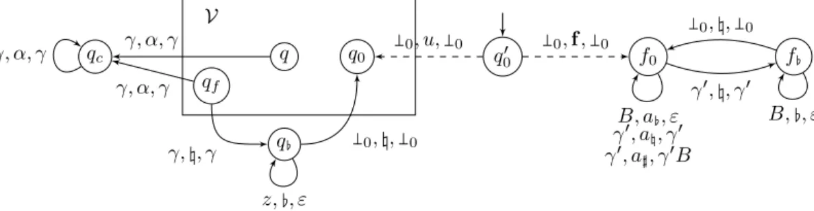
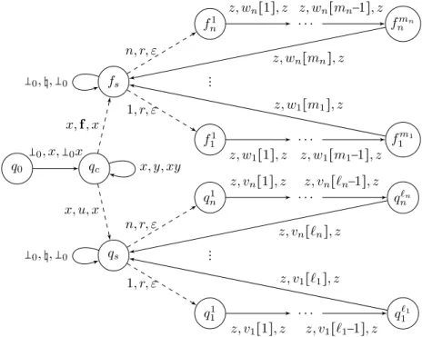
The restriction to visibly pushdown automata is motivated by the unfeasibility of diagnosis for general probabilistic pushdown automata. The undecidability can be obtained by adapting the proof for diagnosis of non-probabilistic pushdown automata [11]. However, in order to show how robust the result is, we rather reduce from the Post Correspondence Problem and prove the undecidability of diagnosability for restricted classes of partially observable probabilistic pushdown automata, see Theorems 23 and 24 in Appendix B.4.

(14)

5 Conclusion

We studied the diagnosability problem for infinite-state probabilistic systems, both from a semantical perspective, and from an algorithmic one when considering probabilistic visibly pushdown automata. A natural research aim is to reduce the complexity gap for the diagnosability of POpVPA (currently EXPTIME-hard and in EXPSPACE). We could also investigate the diagnosability problem for other probabilistic extensions infinite state systems, such as lossy channel systems or VASS. Another research direction would be to consider the fault diagnosis problem for continuous-time probabilistic models, starting with CTMC.

References

1 R. Alur and P. Madhusudan. Visibly pushdown languages. In Proc. STOC’04, pages 202–211. ACM, 2004.

2 N. Bertrand, É. Fabre, S. Haar, S. Haddad, and L. Hélouët. Active diagnosis for probabil-istic systems. In Proc. FoSSaCS’14, volume 8412 of LNCS, pages 29–42. Springer, 2014. 3 N. Bertrand, S. Haddad, and E. Lefaucheux. Foundation of diagnosis and predictability in

probabilistic systems. In Proc. FSTTCS’14, volume 29 of LIPIcs, pages 417–429. Schloss Dagstuhl - Leibniz-Zentrum fuer Informatik, 2014.

4 N. Bertrand, S. Haddad, and E. Lefaucheux. Accurate approximate diagnosability of stochastic systems. In Proc. LATA’16, volume 9618 of LNCS, pages 549–561. Springer, 2016.

5 M. P. Cabasino, A. Giua, and C. Seatzu. Diagnosability of discrete-event systems using labeled Petri nets. IEEE Trans. Automation Science and Engineering, 11(1):144–153, 2014. 6 K. Etessami and M. Yannakakis. Recursive Markov chains, stochastic grammars, and

monotone systems of nonlinear equations. J. ACM, 56(1), 2009.

7 K. Etessami and M. Yannakakis. Model checking of recursive probabilistic systems. ACM

Trans. Computational Logic, 13(2):12, 2012.

8 S. Haar, S. Haddad, T. Melliti, and S. Schwoon. Optimal constructions for active diagnosis. In Proc. FSTTCS’13, volume 24 of LIPIcs, pages 527–539. Schloss Dagstuhl - Leibniz-Zentrum fuer Informatik, 2013.

9 S. Jiang, Z. Huang, V. Chandra, and R. Kumar. A polynomial algorithm for testing diagnosability of discrete-event systems. IEEE Trans. Automatic Control, 46(8):1318–1321, 2001.

10 A. Kučera, J. Esparza, and R. Mayr. Model checking probabilistic pushdown automata.

Logical Methods in Computer Science, 2(1), 2006.

11 C. Morvan and S. Pinchinat. Diagnosability of pushdown systems. In Proceedings of

HVC’09, volume 6405 of LNCS, pages 21–33. Springer, 2009.

12 Y. N. Moschovakis. Descriptive Set Theory. Mathematical Surveys and Monographs. AMS, 2009.

13 M. Sampath, S. Lafortune, and D. Teneketzis. Active diagnosis of discrete-event systems.

IEEE Trans. Automatic Control, 43(7):908–929, 1998.

14 M. Sampath, R. Sengupta, S. Lafortune, K. Sinnamohideen, and D. Teneketzis. Diagnos-ability of discrete-event systems. IEEE Trans. Automatic Control, 40(9):1555–1575, 1995. 15 D. Thorsley and D. Teneketzis. Diagnosability of stochastic discrete-event systems. IEEE

(15)

A

Proofs for Section 3

▸Proposition 5. LetN be a POpLTS. Then N is FF-diagnosable iff N ⊧ P=0(◇ ◻ (f ∧ U)).

Proof. Consider the set of fault-triggering runs:

R= {ρ = q0a0q1. . . ak−1qk∣ ak−1= f ∧ ∀i < k − 1, ai≠ f} .

Write E= {ρ ∈ Ω ∣ ◇ ◻ (f ∧ U)} for the set of runs we are interested in. We further define, for every ρ∈ R, Eρ= {ρ′∈ Ω ∣ ρ ⪯ ρ′∧ρ′⊧ ◻U} and for every n ∈ N, Eρn= {ρ′∈ Ω ∣ ρ ⪯ ρ′∧ρ′⊧ ◻nU}

where ρ⊧ ◻nφ if for every k≤ n, ρ, k ⊧ φ. Observe that E = ⊎ρ∈REρ and that Eρ= ∩n∈NEnρ.

Thus P(E) = ∑ρ∈RP(Eρ) and limn→∞P(Eρn) = P(Eρ).

● Assume first that P(E) > 0. Then, there exists ρ ∈ R such that P(Eρ) > 0. By definition,

for every n> ∣ρ∣oP(FAmbn) ≥ P(Eρ). Thus, N is not FF-diagnosable.

● Assume now that P(E) = 0. So, for every ρ ∈ R, P(Eρ) = 0. Let us pick some ε > 0. Since

F= ⋃n∈NFn, there exists n0 such that for every n≥ n0, P(F ∖ Fn) ≤ ε₃. Let R′= {ρ ∈ R ∣

∣ρ∣o < n0}. Pick a finite subset R′′ of R′ such that ∑ρ∈R′∖R′′P(ρ) ≤ ε

3. Define K = ∣R′′∣.

Let n1 be such that for every n≥ n1 and every ρ∈ R′′, P(Eρn) ≤ ε

3K. Observe now that

for every n≥ n0, FAmbn ⊆ (F ∖ Fn) ∪ ⊎ρ∈R′∖R′′C(ρ) ∪ ⋃ρ∈R′′Eρn. Thus, for every n ≥ n1,

P(FAmbn) ≤ ε₃+ε₃+ K_3Kε = ε. Since ε is arbitrary, N is FF-diagnosable. ◂

▸Proposition 6. LetN be a finitely branching POpLTS. Then N is IA-diagnosable iff

N ⊧ P=0_{(◇ ◻ (U ∧ W)).}

Proof. It is enough to show that ρ∈ Ω is ambiguous if and only if ρ ⊧ ◇ ◻ (U ∧ W). We focus below on correct runs; the case of faulty runs is similar and even simpler.

● Let ρ ∈ CAmb∞. Since ρ is ambiguous, there exists a faulty run ρ′such thatP(ρ′) = P(ρ). Let k0 be such that ρ′_↓k₀ is faulty. Thus for all k≥ k0, firstf(P(ρ_↓k)) ≤ k0and in addition it is

non decreasing. So there exists some k1≥ k0such that for all k≥ k1, firstf(P(ρ↓k)) is constant.

We thus obtain ρ⊧ ◇ ◻ W. Moreover, since ρ ⊧ ◻ U, we conclude that ρ ⊧ ◇ ◻ (U ∧ W). ● Let ρ be a correct run such that ρ ⊧ ◇ ◻ (U ∧ W). Thus there is a position k0such that for

all k≥ k0, ρ, k⊧ W. In particular, by definition of W, for all k ≥ k0, there is a finite signalling

run ρ′(k) such thatP(ρ′(k)) = P(ρ_↓k) and ρ′(k)_↓k

0 is faulty. Consider the tree of these runs ρ

′(k)

by merging the common prefixes. This tree is finitely branching and infinite. By König’s lemma, it must admit an infinite branch, corresponding to a run ρ′with P(ρ′) = P(ρ) and

ρ′_↓k

0 faulty. We deduce that ρ is ambiguous. ◂

Let us recall some standard facts about Borel sets and measures. A set F is closed if and only if F= ⋂n∈NOn where On is a union of cylinders defined by On= {C(ρ) ∣ ∣ρ∣ = n ∧ ∃ρ′∈

F, ρ⪯ ρ′}. Thus an Fσ set F can be written as F = ⋃m_∈N⋂n_∈NOm,nwhere Om,nis a union

of cylinders whose associated paths have length n. Without loss of generality, the sequence of closed sets may be chosen as a non decreasing sequence. The measures we have defined in the core of the paper are regular. In particular, for every measurable set E such that P(E) > 0, there exists a closed set F ⊆ E such that P(F) > 0.

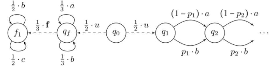
▸Proposition 7. There exists a finitely-branching LTSL and a mask function P such that for every Fσ set E of runs, there exists a POpLTSN = ((L, P), Σo,P) such that:

either N is FA-diagnosable and P_N(E) > 0; orN is not FA-diagnosable and P_N(E) = 0.

Proof. Consider the LTSL = ⟨Q, q0, Σ, T⟩ defined as follows and let the mask function be

(16)

Q= {f1, qf} ∪ {qi∣ i ∈ N}; Σ= {a, b, c, u, f}; T = {(q0, u, qf), (q0, u, q1), (qf, a, qf), (qf, b, qf), (qf, f , f1), (f1, b, f1), (f1, c, f1)} ∪ {(qi, a, qi+1), (qi, b, qi+1)}i≥1. q0 qf f1 q1 q2 . . . 1 2⋅ u 1 2⋅ u 1 3⋅ f 1 3⋅ a 1 3⋅ b 1 2⋅ b 1 2⋅ c (1 − p1) ⋅ a p1⋅ b (1 − p2) ⋅ a p2⋅ b

Figure 6 A family of POpLTS whose underlying LTS has no appropriate characterisation of

FA-diagnosability.

We consider a family of POpLTS, represented in Figure 6, with underlying LTS L. For

p= (pn)n_≥1 a sequence of probabilities, we define the POpLTSNp= ((L, Pp), Σo,P) in

which for every n≥ 1 the probability that b occurs from state qn is Pp(qn, b, qn+1) = pn, and

all other probabilities are independent of p: Pp(q0, u, qf) = Pp(q0, u, q1) = Pp(f1, b, f1) = Pp(f1, c, f1) = 1₂, Pp(qf, a, qf) = Pp(qf, b, qf) = Pp(qf, f , f1) = 1₃.

Observe that limn→∞P(FAmbn) = 0 and P(CAmbn−1) = pn+2

n−1

3n . Therefore, Np is

FA-diagnosable iff limnÐ→∞pn= 0.

Let E be an arbitrary Fσ set. Pick some FA-diagnosableNp i.e. with limnÐ→∞pn= 0. If

Pp(E) > 0 where Ppis the probability measure of this POpLTS, we are done. Assume thus

that Pp(E) = 0. In order to define a second POpLTS, via p′, consider an infinite increasing

sequence {nj}j_≤1 and let for n∉ {nj}j_≤1, p′n= pn and for n∈ {nj}j_≥1, p′n=

1

2. Due to the

sub-sequence p′_n

j = 1

2,Np′ is not FA-diagnosable. The sequence{nj}j≤1 depends on Ppand

will be defined after some preliminary observations.

Let F = {ρ ∣ q0uq1 ⪯ ρ}. Denoting Pp′ the probability measure of the second POpLTS,

observe that Pp′(E ∖ F) = Pp(E ∖ F) = 0. Using the above discussion, the Fσ set E∩ F =

⋃m∈N⋂n∈NOm,nwhere for all m, n, Om,nis a disjoint union of cylinders C(ρ) with ∣ρ∣ = n,

Om,n+1⊆ Om,n and Om,n⊆ Om+1,n. Denote Fm= ⋂n_∈NOm,nFor all m, limn→∞Pp(Om,n) =

Pp(E ∩ Fm) ≤ Pp(E ∩ F) = 0.

● n1 is chosen such that for all n≥ n1, pn≤ 1₂. Observe now that for all nj,

p′nj = 1 2 = 1 2pnj pnj and 1− p ′ nj = 1 2 ≤ 1 − pnj ≤ 1 2pnj (1 − pnj)

By definition of Pp′, since Om,nis a disjoint union of cylinders C(ρ) with ∣ρ∣ = n, applying

inductively the previous inequalities, for all n such that nk< n ≤ nk₊₁ (denoting n0= 0):

Pp′(Om,n) ≤ P

p(Om,n)

2k_∏

1≤j<kpnj

. (1)

● Assume that we have chosen n1, . . . , nk. Since limn_→∞Pp(Ok,n) = 0, there exists nk₊₁> nk

such that Pp(Ok,nk+1) ≤ ∏1≤j≤kpnj. We choose such an index.

Equation 1 now implies that for all m≤ k, Pp′(Om,nk+1) ≤ Pp′(Ok,nk+1) ≤ 1

2k. Thus for all m, Pp′(Fm) = limk_→∞Pp′(Om,nk+1) = 0. Since E ∩ F = ⋃m∈NFm, Pp′(E ∩ F) = 0 and so

(17)

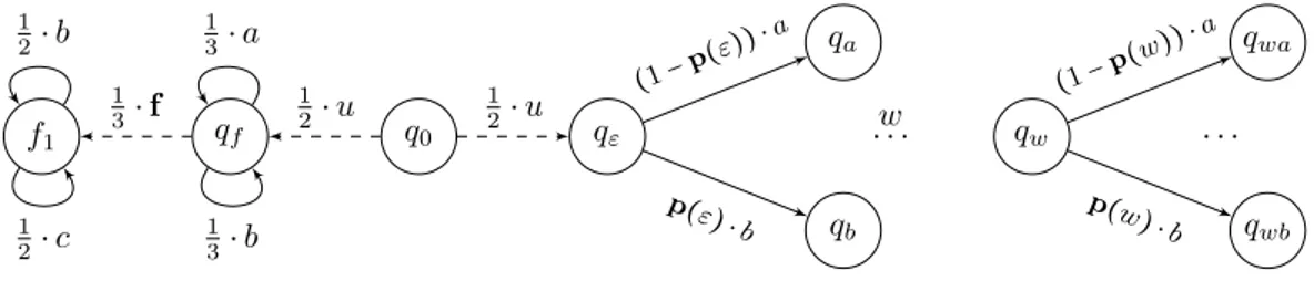
▸Proposition 8. There exists a finitely-branching LTSL and a mask function P such that for every Borel set E of runs, there exists a POpLTSN = ((L, P), Σo,P) such that:

either N is FA-diagnosable and P_N(E) = 0; orN is not FA-diagnosable and P_N(E) > 0.

Proof. Consider the LTSL = ⟨Q, q0, Σ, T⟩ defined as follows, and let the mask function be

defined by: P(u) = P(f) = ε and P is the identity over the other events.

Q= {f1, qf, q0} ∪ {qw∣ w ∈ (a + b)∗}; Σ= {a, b, c, u, f}; T= {(q0, u, qf), (q0, u, q1), (qf, a, qf), (qf, b, qf), (qf, f , f1), (f1, b, f1), (f1, c, f1)} ∪ {(qw, a, qwa), (qw, b, qwb)}w∈(a+b)∗. q0 qf f1 qε qw qwa qwb qa qb w . . . . . . 1 2⋅ u 1 2⋅ u 1 3⋅ f 1 3⋅ a 1 3⋅ b 1 2⋅ b 1 2⋅ c (1− p (ε)) ⋅ a p(_ε) ⋅_b (1− p (w)) ⋅ a p(_w ) ⋅ b

Figure 7 Another family of POpLTS whose underlying LTS has no appropriate characterisation

of FA-diagnosability.

We consider a family of POpLTS, represented in Figure 7, with underlying LTSL, para-meterised by a mapping p∶ (a + b)∗→ (0, 1). Let Np= ((L, Pp), Σo,P) be the POpLTS such

that the probability that b occurs from state qwis P(qw, b, qwb) = p(w), and all other

probab-ilities are independent from p: Pp(q0, u, qf) = Pp(q0, u, q1) = Pp(f1, b, f1) = Pp(f1, c, f1) = 1₂, Pp(qf, a, qf) = Pp(qf, b, qf) = Pp(qf, f , f1) = 1₃. In the sequel, for convenience, we also write p(w, b) for p(w), and define p(w, a) = 1 − p(w), so that P(qw, a, qwa) = p(w, a).

Word w can be decomposed into letters w= w[1] . . . w[n], and we give notations for factors:

w[1, k] = w[1] . . . w[k] with the convention that w[1, 0] = ε. Finally we define pp(w) =

∏1≤k≤np(w[1, k − 1], w[k]), as the probability to read w from qε. Since limn→∞P(FAmbn) =

0 and P(CAmbn−1) = ∑_{∣w∣=n−1}p(w, b) + 2

n−1

3n , we deduce that Np is FA-diagnosable iff

limnÐ→_∞∑_{∣w∣=n−1}p(w, b) = 0.

Let E be an arbitrary measurable set. Pick some POpLTS Np which is FA-diagnosable,

i.e. with limnÐ→_∞∑_{∣w∣=n−1}p(w, b) = 0. If Pp(E) = 0 where Pp is the probability of this

POpLTS, we are done. Assume therefore that Pp(E) > 0. Let F = {ρ ∣ q0uqε⊑ ρ} be the set

of runs starting with a u-transition to qε. Denoting Pp′ the probability measure of any other

POpLTSNp′, observe that Pp′(E ∖ F) = Pp(E ∖ F). So, if Pp(E ∖ F) > 0, then by picking

any non FA-diagnosable (L, Pp′), we are done. So assume Pp(E ∖ F) = 0 which implies

Pp(E ∩ F) > 0. Using our recalls, there exists a closed set G ⊆ E ∩ F with Pp(G) > 0.

If G= F then Pp′(G) = Pp(G) = 1₂. In this case, we can therefore conclude by picking any

non FA-diagnosable POpLTSNp′.

Assuming G⊊ F, since G is closed, there is some cylinder C(ρ) with ρ = q0uqε. . . qw such

that G∩C(ρ) = ∅. Then we define the POpLTS Np′ as the POpLTSNpexcept that for every

w⪯ w′ and every x∈ {a, b}, p′(w′, x) = 1₂. Thus for every n≥ ∣w∣, ∑_∣w′_∣=np′(w′, b) ≥ Pp₂(ρ).

(18)

B

Details and proofs for Section 4

B.1 Formal definitions

Here we give formal definitions omitted in the core of the paper due to space constraints. More precisely given a POpVPAV, we define its estimate VPA A(V), its enlarged VPA ̂V and their synchronised product.

Let µ∈ {g, c, f} we write (q, γ)Ô⇒o µ(q′, w) with o ∈ Σo if when µ= g (resp. c, f), there

exists a general (resp. correct, faulty) run of transitions starting from(q, γ) to (q′, w) such

that all transitions are unobservable except the last one labelled by e with P(e) = o. Let

ρ be such a run then we also write (q, γ)Ô⇒ρ µ(q′, w) All transitions of such runs are local

except the last one whose type depends on the type of o.

▸Definition 16. Given⟨V, P, Σo⟩ a POpVPA with V = (Q, Σ, Γ, δ, P), its estimate VPA is

the deterministic VPAA(V) = (Qe, Σo, Γe, δe) defined by:

Qe= {run} ⊎ (2Γ×(Tg×Q)2∖ ∅) is the set of states with initial state q₀e= run;

Γe_{= 2}(Γ×Tg×Q)2_{∖ ∅ is the stack alphabet with set of bottom stack symbols Γ}e

= 2Init∖ ∅

where Init= {0,X,q

0,U,q0 ∣ (X, q) ∈ Tg × Q} and initial stack symbol 

e

0= {

q0,U,0

q0,U,0};

The transition relation δe _{is defined as follows.}

local transitions (run, bel, o, run, bel′) ∈ δe if:

β,U,r α−,U,q− ∈ bel

′_{iff there exists} α,U,q

α−,U,q−∈ bel and (q, α) o

Ô⇒c(r, β).

If W occurs in bel, _αβ,W,r−_,X,q−∈ bel′iff there exists _αα,W,q−_,X,q− ∈ bel and (q, α)

o

Ô⇒g(r, β).

If W occurs in bel, _αβ,V,r−_,X,q−∈ bel′iff

(1) there exists _αα,U,q−_,U,q−∈ bel and (q, α)

o

Ô⇒f (r, β) or

(2) there exists _αα,V,q−_,X,q−∈ bel and (q, α)

o

Ô⇒g(r, β).

If W does not occur in bel, _αβ,W,r−_,X,q− ∈ bel′iff

(1) there exists _αα,U,q−_,X,q−∈ bel and (q, α)

o

Ô⇒f (r, β) or

o

Ô⇒g(r, β).

push transitions (run, bel, o, run, bel′bel′′) ∈ δe _if: β−,U,r

α−,U,q− ∈ bel

′_and β,U,r β−,U,r ∈ bel

′′_{iff there exists} α,U,q

α−,U,q− ∈ bel and (q, α) o

Ô⇒c(r, β−β).

If W occurs in bel, _αβ−−,X,q,W,r−∈ bel′and β,W,r

β−,W,r ∈ bel′′ iff

there exists _αα,W,q−,X,q− ∈ bel and (q, α) o

Ô⇒g(r, β−β).

If W occurs in bel, _αβ−−_,X,q,V,r−∈ bel′and _ββ,V,r−_,V,r ∈ bel′′ iff

o

Ô⇒f (r, β−β) or

o

Ô⇒g(r, β−β).

If W does not occur in bel, _αβ−−,X,q,W,r− ∈ bel

′_and β,W,r β−,W,r ∈ bel

′′ _iff

o

Ô⇒f (r, β−β) or

o

Ô⇒g(r, β−β).

pop transitions (run, bel, o, `, ε) ∈ δewith `∈ Qe∖ {run} if:

U,r

α−,U,q− ∈ ` iff α,U,q

α−,U,q− ∈ bel and (q, α) o

Ô⇒c(r, ε).

If W occurs in bel, _α−W,r,X,q−∈ ` iff there exists α,W,q

α−,X,q− ∈ bel and (q, α) o

Ô⇒g(r, ε).

If W occurs in bel, _α−V,r,X,q−∈ ` iff

(1) there exists _αα,U,q−,U,q−∈ bel and (q, α) o

Ô⇒f (r, ε) or

o